Machine Learning and Parallelism in the Reconstruction of LHCb
and its Upgrade
MichelDe Cian1,aon behalf of the LHCb collaboration 1Physikalisches Institut der Universität Heidelberg, Germany
Abstract.The LHCb detector at the LHC is a general purpose detector in the forward region with a focus on reconstructing decays of c- and b-hadrons. For Run II of the LHC, a new trigger strategy with a real-time reconstruction, alignment and calibration was employed. This was made possible by implementing an offline-like track reconstruction in the high level trigger. However, the ever increasing need for a higher throughput and the move to parallelism in the CPU architectures in the last years necessitated the use of vectorization techniques to achieve the desired speed and a more extensive use of machine learning to veto bad events early on. This document discusses selected improvements in computationally expensive parts of the track reconstruction, like the Kalman filter, as well as an improved approach to get rid of fake tracks using fast machine learning techniques. In the last part, a short overview of the track reconstruction challenges for the upgrade of LHCb, is given. Running a fully software-based trigger, a large gain in speed in the reconstruction has to be achieved to cope with the 40 MHz bunch-crossing rate. Two possible approaches for techniques exploiting massive parallelization are discussed.
1 Introduction
For Run II of the LHC, LHCb adopted a new trigger strategy with a real-time reconstruction, align-ment and calibration. This allows to directly use the output of the trigger reconstruction to perform physics analyses [1]. To achieve this goal, the track reconstruction in the high-level software trigger (HLT, online) and offline had to be unified, to already obtain the best performance for the real-time alignment and calibration online. Several strategies were employed. A new sequence for the track reconstruction was implemented, which lead to a large speed up. This will be discussed in Section2. For very computing intensive parts of the code, parallelization in the form of SIMD (single instruc-tion, multiple data) instructions were used that lead to a large gain in time, see Section3. Furthermore, machine learning methods were employed to reject tracks which do not originate from a real particle (Section4). Section5then discusses the total gain in timing.
The upgraded LHCb detector, which will start taking data in 2020, will use a fully software-based trigger to cope with the 40 MHz bunch crossing rate. In Section6 two possible strategies and one technical aspect on how to perform track reconstruction in this high multiplicity environment are discussed.
2 The LHCb detector
The LHCb experiment (see Figure1) is dedicated to the study of beauty and charm hadron decays with special attention paid toCPviolating phenomena as well as searches for physics beyond the Standard Model through rare decays. Since the beauty production cross-section is dominated by gluon fusion, which occurs in the forward region, the LHCb detector is a single-arm forward spectrometer with a pseudorapidityη spanning the range 1.8 < η < 4.9 [2,3]. The detector includes a high-precision tracking system consisting of a silicon-strip vertex detector (VELO) surrounding the ppinteraction region, a large-area silicon-strip detector (TT) located upstream of a dipole magnet with a bending power of about 4 Tm, and three stations of silicon-strip detectors (IT) and straw drift tubes (OT) placed downstream of the magnet. The tracking system provides a measurement of the momentum pof charged particles with a relative uncertainty that varies from 0.5% at low momentum to 1.0% at 200 GeV/c. The minimum distance of a track to a proton-proton collision, the impact parameter, is measured with a resolution of (15+29/pT)μm, wherepTis the component of the momentum trans-verse to the beam, in GeV/c. Different types of charged hadrons are distinguished using information from two ring-imaging Cherenkov detectors (RICH1, RICH2). Photons, electrons and hadrons are identified by a calorimeter system consisting of scintillating-pad (SPD) and preshower detectors (PS), an electromagnetic calorimeter (ECAL) and a hadronic calorimeter (HCAL). Muons are identified by a system composed of alternating layers of iron and multi-wire proportional chambers (MUON).
The LHCb coordinate system is a right handed Cartesian system with the origin at the interaction point. Thex-axis is oriented horizontally towards the outside of the LHC ring, they-axis is pointing upwards with respect to the beam line and thez-axis is aligned with the beam direction.
The online event selection is performed by the trigger, which is composed of three stages: a stage implemented in hardware known as Level 0 (L0) and two stages implemented in software called High-Level-Trigger (HLT1 and HLT2). The HLT1 performs a partial reconstruction of the candidates. In this stage all requirements are inclusive, which means that the selection is applied only to subset of the final state particles. The HLT2 contains both inclusive and exclusive algorithms which are more time-consuming but provide a more precise reconstruction. Exclusive algorithms are used to select a specific decay at the trigger stage.
M1
M3 M2
M4 M5 RICH2
HCAL ECAL SPD/PS Magnet
z 5m
y
5m
10m 15m 20m
TT
T1T2
T3
Vertex Locator
MkZ\dbg`
Particle ID
p
p
2.1 Track types
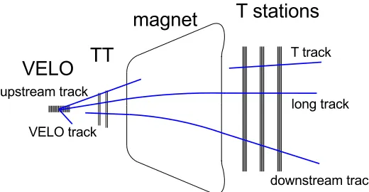
With its three tracking detectors, several track types can be reconstructed in LHCb, see Figure2. The most important category are so-called long tracks, which traverse the full tracking systems and therefore deposit charge in the VELO, the T-stations and potentially also in TT. They are formed from daughters of promptly decaying particles and from daughters of b- and c-hadrons, which only travel a couple of mm before their decay. The other important type are so-called downstream tracks. They originate from daughters of long-living particles, which decay after the VELO and therefore are only reconstructed in TT and the T-stations. Long tracks are reconstructed using two dedicated algorithms. The first, called forward tracking, starts with VELO [4] or upstream tracks [5] and tries to find corresponding clusters in the T-stations [6]. The second, called track matching, uses tracks in the VELO and the T-stations [7] (called T tracks) as starting point and tries to match them in the magnet region [8,9]. Downstream tracks are reconstructed by using tracks in the T-stations as starting point and extrapolating them back through the magnet [10].
Figure 2. Track types in LHCb. Long tracks and downstream tracks are used for physics analyses, the other types either serve as a component of another track type or are used for detector studies.
2.2 Run II track reconstruction sequence
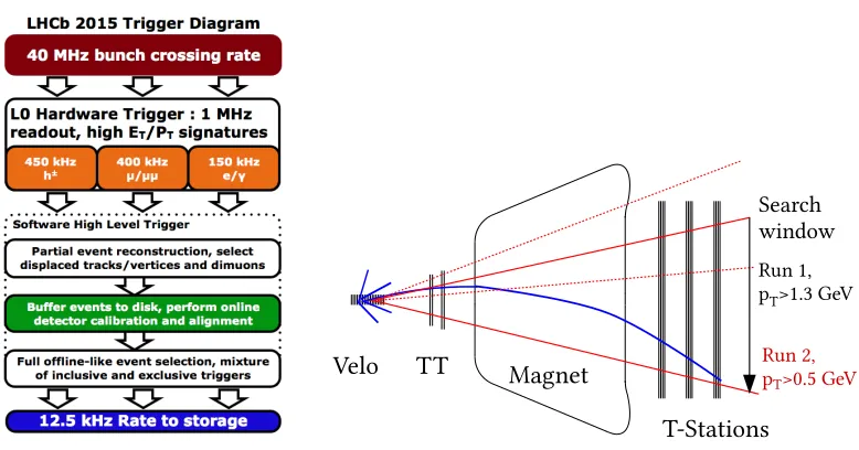
The run II track reconstruction sequence is split in an HLT1 and HLT2 part (see left part of Figure3). In HLT1, all VELO tracks are reconstructed. These VELO tracks are fitted with a simplified Kalman filter (allowing for a single scattering at the sensor planes) and are then used to find the primary vertices. The VELO tracks are also extrapolated to TT, where clusters around the extrapolation are searched for. Due to the fringe field of the magnet this provides a first estimate of the sign of the charge. The tracks are then propagated through the magnet to the T-stations, searching for corre-sponding clusters, such that all tracks with a transverse momentum larger than 500 MeV/care found (right part of Figure3). The tracks found are fitted with a Kalman Filter.
In HLT2, the HLT1 reconstruction part is repeated first. Then all VELO tracks which could not be made into long tracks are again propagated to the T-stations, however without requiring clusters in TT or a cut on the transverse momentum. In addition, T tracks are reconstructed and combined with VELO tracks, to form long tracks, and with clusters in TT, to form downstream tracks. All tracks are fitted with a Kalman filter and clones from the different algorithms are removed.
Search window
Run 1, pT>1.3GeV
Run 2, pT>0.5GeV
Ve
l
o TT
T-
S
t
a
t
i
o
ns
Ma
g
ne
t
Figure 3.Scheme of the trigger for Run II of LHCb (left). Scheme for the reconstruction of long tracks in Run I and Run II (right). Note that thepTthreshold could be lowered in Run II, allowing for a higher physics yield.
3 SIMD in LHCb
3.1 The need for speed
Even though the new sequence resulted in a reduction in execution time, a further decrease was needed. In order to achieve this, SIMD instructions were introduced. There were two main problems. Most of the code of the LHCb track reconstruction was written several years ago and was not adapted to make use of parallelization natively. Furthermore, a large part of the pattern recognition code con-sists of selecting the right clusters, tracks, etc., and therefore makes heavy use of branching. SIMD uses vector instructions, meaning that basic mathematical operations like addition and multiplication can be executed in parallel on more than one value. However, this only works if it is guaranteed that all values actually will be computed, and not discarded due to choosing the wrong branch. It is there-fore best suited for those parts of the reconstruction code, where purely mathematical computations play a large role in the total time consumption.
3.2 Hough transform in forward tracking
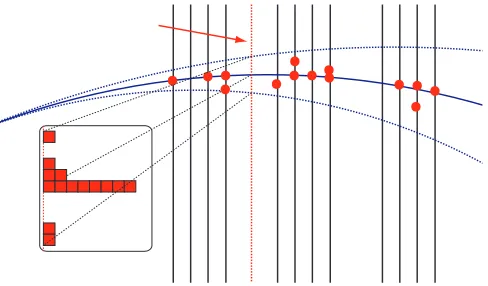
In the forward algorithm, a VELO (or upstream) track, defining the position and the slopes, is matched to a single cluster in the T-stations. This completely defines all five parameters of the track. All clusters that belong to the same track should therefore accumulate in the same point when projected to a plane parallel to the tracking stations at a given point inz(“Hough plane”), assuming that the track model is correct and neglecting multiple scattering (see Figure4). This accumulation can then be used to find valid track candidates. The projection of the cluster from its position in the detector plane to the Hough plane uses a third order polynomial, whose coefficients are derived in an iterative way. For each VELO track, all clusters have to be projected exactly once and they are independent of each other, which makes it an ideal case for SIMD instructions.
The overall reduction in time of using SIMD compared to processing the clusters sequentially is about 40%, which is close to the theoretical maximum of 50%, when using SSE2 and double values. The difference stems from the fact that the positions of the clusters are in a layout which needs to be made usable for SIMD first.
Figure 4. Illustration of the Hough transform. Clusters belonging to the same track (solid blue line) will ac-cumulate around the same point in the Hough plane (red-dashed line) when being projected from their original position. Other clusters will be distributed randomly.
3.3 Computations in the Kalman Filter
1 2 3 4 2 5 4 5 6
7 8 9 10
7 8 9 1 2 3 4 5 6 7 8 9 10 11 12 13 14 15 16 1 5 9 13 2 6 10 14 3 7 11 15 4 8 12 16 1 2 4 7 3 2 5 8 4 5 6 9 10 7 8 9
1 2 3 4
1
2
3
4
=
*
+
*
+
*
+
*
Figure 5.Illustration of the multiplication of three matrices,F·C·FT. The second row shows how the
multi-plication of the last two matrices can be decomposed in the sum of multimulti-plications of a row-vector with a scalar value, which can be exploited with SIMD instructions.
4 Machine learning
Due to its long lever arm between the tracking stations before and after the magnet, a relatively large fraction of reconstructed tracks are “fake”, i.e. they do not correspond to a real charged particle having crossed the detector. In Run I, a cut on theχ2/ndof of the tracks after the Kalman filter was applied. Later, the user of the data could select tracks with a low fake-probability by cutting on a quantity called “ghost probability”. This classifier was based on a neural net.
Approximately 22% of all reconstructed long tracks after the cut onχ2/ndof were estimated to be fake in Run II. To further reduce this rate in the reconstruction, the idea was to use the ghost probability classifier directly in the final selection of tracks .
For Run II, the ghost probability is still based on a neural net, however it only uses variables as input which do not consume much computing power in the calculation. In total, 21 input variables are used. Most of them are taken from the result of the Kalman filter, like the overallχ2/ndof, but also theχ2/ndof of segments of the track, for example the TT – T-station segment. These segments might be more sensitive to detecting so called matching ghosts. They occur when a real VELO or upstream track and a real track in the T-stations are matched, although originating from different particles. The neural net consists of one hidden layer with 26 nodes. No gain in performance was seen by training a deep neural net. Likewise no gain was seen by using human assisted learning, i.e. forming new variables from the raw quantities as an input to the neural net.
To further speed up the calculation, the activation function of the neural net was chosen to be 1/√1+x2. This decreased the time consumption by a factor of 50 compared to using the hyperbolic tangent as activation function, which was the default in the Run I classifier.
] 2 [MeV/c π K m
1800 1850 1900
)
2
candidates / (4 MeV/c
0 500 1000 1500 2000 2500 3000 3500 LHCb preliminary π K → 0 all D fakes ] 2 [MeV/c π π m
480 500 520
)
2
Candidates / (10 MeV/c
0 500 1000 1500 2000 π π → S all K fakes π π → s selected K LHCb preliminary long tracks
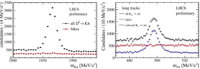
Figure 6.Performance of the ghost probability classifier for long tracks andD0→Kπ(left) andK
S→ππ(right) decays. The rejected events are shown in red and show no peaking structure, meaning that no signal is lost with the cut on the ghost probability.
5 Total gain in timing
In addition to the presented points, many small-scale optimisations were performed in all the pattern recognition algorithms and in the Kalman filter, for example more efficient calculations or better use of the C++11 standard. The total speed-up, when comparing the reconstruction sequence in Run I and Run II, was a factor of 2, without any loss in performance. To achieve the same physics results without any modification of the code would have resulted in buying more machines for the HLT farm, whose total cost would have been several million Swiss francs.
6 Track reconstruction in the upgrade of LHCb
The LHCb detector will be upgraded in the long shutdown 2 of the LHC and restart taking data in 2020 at an instantaneous luminosity of 2·1033cm−2s−1, which is about a factor of 5 more than the current instantaneous luminosity. At this luminosity, the rate of potentially interesting physics events would be too high for the L0 hardware trigger to handle. The idea is therefore to have only a software trigger which runs at the full bunch-crossing frequency. In order to achieve this goal, the tracking system needs to be replaced. The current VELO, a silicon strip detector, will be replaced by a pixel-based solution with a very high track reconstruction efficiency [11]. The TT-station before the magnet will be replaced by a silicon strip detector with a fine granularity [12]. The tracking stations behind the magnet will consist of 12 layers of a scintillating fiber tracker, which is read out by silicon photomultipliers [12].
The overall time available for track reconstruction is expected to be about 15 ms per event. This places strong constraints on all pattern recognition algorithms and the track fitter. The only way to achieve this goal is to exploit parallelisation, either using CPUs, or using other architectures, for example GPUs or Intel Xeon Phi. The main question is not only about the best raw performance, but mainly about the best performance for the amount of invested money.
6.1 Cellular automaton tracking
clusters have to be found in the other layers. One idea to perform this track reconstruction is to use a cellular automaton approach (see Ref. [13] for an example). First, tracklets between the twoxlayers in all three T-stations are reconstructed. Then stereo hits are added, leading to so-called “stubs”. These stubs now need to be connected between the three stations: Three-stations stubs are preferred over two-station stubs, as the latter are more likely to be fake tracks.
To test the efficiency of this approach (irrespective of the time consumption), a CPU implementa-tion was written for the Run II detector. The track reconstrucimplementa-tion efficiency of the cellular automaton approach is within a couple of percent of the nominal algorithm to reconstruct T tracks, where it has to be taken into account that the Run II algorithm has undergone extensive tuning over several years. The next step is now to port the algorithm to a GPU to test the performance not only for track reconstruction efficiency, but mainly for time consumption.
6.2 VELO tracking with GPUs
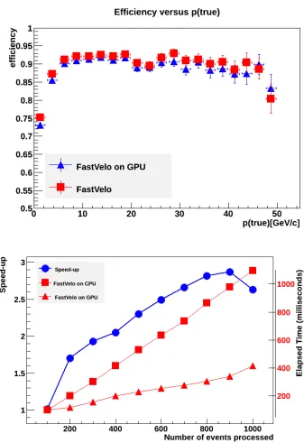
Another approach to gain experience with GPUs is to take an existing track reconstruction algo-rithm (in this case for the VELO standalone tracking), and to port it to a GPU, using the CUDA language [14]. This algorithm runs in “parasitic” mode in the monitoring farm of the HLT, mean-ing that it can be tested in real data takmean-ing conditions. While the efficiencies between the CPU and the GPU implementations are very similar, the GPU, as expected, shows an advantage when several events can be prepared in such a way that they can be processed in parallel, see Figure7.
6.3 Structure of arrays
In order to optimally exploit SIMD instructions, the data needs to be provided in a “vectorization-friendly” way. At the moment, most classes in LHCb are arranged in an array-of-structures. For example, a cluster in a tracking detector is represented (in a simplified way) with a class “cluster” and holds three members, its coordinates x, y,z. A set of clusters therefore is arranged as an array of the cluster class. However, when using SIMD instructions, for example to calculate something with thex-coordinates only, the values are not sequential in memory. This prevents SIMD to process them simultaneously. The solution is to arrange the clusters in three arrays, each of them holding one coordinate only. This is less intuitive, but accessing thex-coordinates would mean accessing values which are next to each other in memory, greatly benefitting vectorization with SIMD.
Studies have started in LHCb that exploit the structure-of-array arrangement to speed up critical parts of the code.
7 Conclusion
References
[1] Aaij, R. et al (2016),arXiv:1604.05596
[2] Alves, A. et al., JINST3, S08005 (2008)
[3] Aaij R. et al, Int. J. Mod. Phys. A30, 1530022 (2015),
http://www.worldscientific.com/doi/pdf/10.1142/S0217751X15300227
[4] O. Callot, Tech. Rep. LHCb-PUB-2011-001. CERN-LHCb-PUB-2011-001, CERN, Geneva (2011),https://cds.cern.ch/record/1322644
[5] E.E. Bowen, B. Storaci, M. Tresch, Tech. Rep. LHCb-PUB-2015-024. CERN-LHCb-PUB-2015-024. LHCb-INT-2014-040, CERN, Geneva (2016),
https://cds.cern.ch/record/2105078
[6] O. Callot, S. Hansmann-Menzemer, Tech. Rep. LHCb-2007-015. CERN-LHCb-2007-015, CERN, Geneva (2007),https://cds.cern.ch/record/1033584
[7] O. Callot, M. Schiller, Tech. Rep. LHCb-2008-042. CERN-LHCb-2008-042, CERN, Geneva (2008),https://cds.cern.ch/record/1119095
[8] M. Needham, J. Van Tilburg, Tech. Rep. LHCb-2007-020. CERN-LHCb-2007-020, CERN, Geneva (2007),https://cds.cern.ch/record/1020304
[9] M. Needham, Tech. Rep. LHCb-2007-129. CERN-LHCb-2007-129, CERN, Geneva (2007),
https://cds.cern.ch/record/1060807
[10] O. Callot, Tech. Rep. LHCb-2007-026. CERN-LHCb-2007-026, CERN, Geneva (2007),
https://cds.cern.ch/record/1025827
[11] LHCb Collaboration, Tech. Rep. CERN-LHCC-2013-021. LHCB-TDR-013, CERN, Geneva (2013),https://cds.cern.ch/record/1624070
[12] LHCb Collaboration, Tech. Rep. CERN-LHCC-2014-001. LHCB-TDR-015, CERN, Geneva (2014),https://cds.cern.ch/record/1647400
[13] I.S. Kulakov, S.A. Baginyan, V.V. Ivanov, P.I. Kisel, Phys. Part. Nuclei Letters10, 162 (2013) [14] A. Badalov et al., Tech. Rep. LHCb-PUB-2014-034. CERN-LHCb-PUB-2014-034, CERN,