Eliciting Human Judgment for Prediction Algorithms
Rouba Ibrahim
School of Management, University College London, [email protected] Song-Hee Kim
Marshall School of Business, University of Southern California, [email protected] Jordan Tong
Wisconsin School of Business, University of Wisconsin-Madison, [email protected] August 3, 2020
Even when human point forecasts are less accurate than data-based algorithm predictions, they can still help boost
per-formance by being used as algorithm inputs. Assuming one uses human judgment indirectly in this manner, we propose
changing the elicitation question from the traditional direct forecast (DF) to what we call the private information
adjust-ment (PIA): how much the human thinks the algorithm should adjust its forecast to account for information the human has
that is unused by the algorithm. Using stylized models with and without random error, we theoretically prove that human
random error makes eliciting the PIA lead to more accurate predictions than eliciting the DF. However, this DF-PIA gap
does not exist for perfectly consistent forecasters. The DF-PIA gap is increasing in the random error that people make
while incorporating public information (data that the algorithm uses) but is decreasing in the random error that people
make while incorporating private information (data that only the human can use). In controlled experiments with students
and Amazon Mechanical Turk workers, we find support for these hypotheses.
Key words: laboratory experiments, behavioral operations, random error, elicitation, forecasting, prediction, discretion,
expert input, private information, judgment, aggregation
1.
Introduction
Because of increased access to data and advancements in machine-learning algorithms, a common opera-tional improvement initiative is to replace human forecasters with data-driven prediction algorithms. For example, in our motivating setting, a hospital needs surgery duration forecasts to schedule operating room use, which costs$2,190per hour on average (Childers and Maggard-Gibbons 2018). Using surgery dura-tion data from that hospital, Ibrahim and Kim (2019) show that physicians’ mean absolute percent forecast error was 33%, whereas algorithms based on available patient and surgery data reduced that error to 29%.
Nevertheless, even if humans are not better than algorithms head-to-head, their judgments can still help. In the above example, the hospital could improve predictive accuracy even further, to under 27%, by using the physicians’ forecasts as an input (along with the other data) to the algorithm. In other words, the best forecasts often come not from replacing humans with algorithms, but from combining them.
directly, but ratherindirectly, in an algorithm, should we elicit something else besides point forecasts? If so, what human judgment should we elicit, and why might it work better?
We theorize that the primary reason why humans add value to algorithms is that they have access to private information that the algorithm does not use, for example, because it is not in the database or there are not sufficient historical training data for the algorithm to effectively use it. Therefore, we consider whether, rather than asking for a human’sdirect forecast(DF), it may be better to instead ask about her judgment of this private information’s impact (even if the system designer does not know what this private information is ahead of time). Specifically, we propose the idea of eliciting theprivate information adjustment(PIA)— how much the human thinks the algorithm should adjust its forecast to account for the information that only the human has.
Using stylized models (§2), we theorize that the PIA leads to more accurate predictions than DF only if there is human random error. That is, from a predictive accuracy perspective, there is no difference between eliciting a DF or the PIA if people are perfectly consistent in how they use information to make a forecast. However, if they are inconsistent, then the PIA should help algorithms more than the DF. Furthermore, the models shed light on how random error creates this difference by predicting which environmental conditions would lead to greater differences in performance. Namely, they show that the PIA’s advantage, relative to DF, is larger when “public” data—the data that the algorithm uses—are complicated for the human to process but smaller when the human’s private information is complicated to process instead.
To test these hypotheses regarding the difference in performance between DF and PIA, we conducted controlled experiments in which we elicited human judgments for 50 simulated surgery durations based on predictive data. We told our participants that the hospital’s algorithm had access to only some of the data (“public information”) and that only the participant had access to the other data (“private information”). In one condition, we elicited judgment by asking for the participant’s DF for each surgery, while in the other, we elicited the participant’s PIA for each surgery. Then, for each condition, we calibrated prediction algorithms using the first 35 surgeries and tested their predictive performance using the last 15 surgeries.
complex. Finally, in§5, we discuss why private information exists in practice, implications of our findings, and opportunities for future research.
We contribute to four main bodies of research. Management science researchers have recognized the potential value in integrating human judgment with forecasting algorithms (see Arvan et al. 2019 for a review). Humans often possess so-called “domain knowledge”: better and more up-to-date information than what statistical models use (see §3 of Lawrence et al. 2006). Such domain knowledge is the generally accepted explanation for why human judgmental forecasting sometimes even outperforms statistical models in practice (see Lawrence et al. 2000 for sales forecasting and Alexander Jr 1995 for earnings forecasting). The two most common integration approaches are to make judgmental adjustments to an algorithm’s point forecast (e.g., see Carbone et al. 1983, Fildes et al. 2009) or to combine separate human and algorithm point forecasts (e.g., see Blattberg and Hoch 1990, Goodwin 2000). We contribute by examining a differ-ent human elicitation question from the point forecast. Notably, our proposed method isnot equivalent to judgmental adjustments because we use the PIA as an input for the prediction algorithm. In fact, in our experiments, using PIA responses to adjust algorithm forecast outputs yields poor predictive performance.
A stream of behavioral operations management research studies thesystem design implications of human random error. For example, the best way to design contracts (Su 2008, Ho and Zhang 2008), queues (Huang
et al. 2013, Tong and Feiler 2017), or auctions (Davis et al. 2014) changes once the system designer consid-ers human random error. Most closely related to our paper is Kremer et al. (2016). They show that human random error causes eliciting human forecasts in a top-down fashion to be more effective in some environ-ments but bottom-up forecasting to be more effective in others. We contribute by showing how a forecasting system’s elicitation design impacts performance once one considers human random error, even if it has no effect without human random error.
Researchers in judgment and decision making have made advancements in developing strategies to improve human judgment accuracy. Perhaps the most well-known idea is to harness the “wisdom of crowds”
Lastly, studying the benefit of incorporating discretion from humans with local knowledge in opera-tional decision makinghas been an emerging topic of study in operations management. Various application domains have been considered, such as capacity decisions in service operations (Campbell and Frei 2011), sales forecasting (Osadchiy et al. 2013), price setting (Phillips et al. 2015), hospital unit admission decisions (Kim et al. 2015), and product removal decisions in retail stores (Kesavan and Kushwaha 2020).
2.
Theory Development
In this section, we leverage simple mathematical models to compare the theoretical performance of a pre-diction algorithm that uses human DF and one that uses human PIA. Specifically, our focus is on showing that the difference in performance depends critically on whether or not we assume the forecaster suffers from random error. Our theoretical development is agnostic about the exact sources of this random error and does not attempt to provide a detailed description of the psychology of prediction. Rather, the point of the models is to clearly demonstrate that including random error in the forecast is sufficient to generate differences between DF and PIA. We use these results to motivate two hypotheses about whether and how eliciting the PIA will be more effective than DF.
2.1. Surgery Duration Assumptions
We assume an actual surgery duration,Y, is a random variable defined by the linear model
Y =v+ X i∈P∪I
wiXi+, (1)
where we separate the public factors, denoted by the index setP, from the private factors, denoted by the index setI. In (1),is an error term, withE[] = 0, which represents true environmental random shocks, i.e.,
random variations that are impossible to predict even with all public and private information. We assume thatand(Xi)i∈P∪I are mutually independent.
2.2. DF and PIA Are Equivalently Effective with Consistent Forecasters (No Random Error)
We define DF and PIA for theconsistent forecasterwho does not suffer from random error as follows:
DF∗=v∗+ X i∈P∪I
w∗iXi and PIA∗=
X
i∈I
w∗iXi. (2)
Here, we assume that v∗ andw∗
i, fori∈ P ∪ I, aredeterministic, though not necessarily known by the algorithm a priori. (Note that they can be any constants and are not necessarily “optimal”. For example, settingwi∗= 0is equivalent to assuming humans do not use that information.) Define the best-fitting models ofY given the public factors andDF∗orPIA∗using linear regression:
(Model-DF∗) M
DF∗=α0+ X
i∈P
(Model-PIA∗) MPIA∗=γ0+ X
i∈P
γiXi+βPIA∗PIA∗. (4)
Then, the following proposition holds. We relegate the proofs of all propositions to the Appendix.
PROPOSITION1. Model-DF∗and Model-PIA∗yield the same predictions.
That is, with consistent forecasters, predicting surgery durations using DFs as model inputs yields the same predictions as using PIAs as model inputs; the two elicitation methods are equivalent from the algorithm’s perspective.
2.3. PIA Outperforms DF with Inconsistent Forecasters (Random Error)
Next, we define DF and PIA for theinconsistent forecasterwho does suffer from random error:
DFb=vb+ X i∈P∪I
WibXi and PIAb=
X
i∈I
WibXi. (5)
Here, we assume thatWb
i arerandom variableswithE[W b i] = ¯w
b
i and Var[W b
i]>0. We also assume that Wb
i andXi are all mutually independent, fori∈ P ∪ I. Thus, in contrast to (2), (5) captures inconsisten-cies or random error in assigning weights to each factor. For example, these random weights could reflect inconsistencies in the encoding of information, memory retrieval, aggregation of multiple factors, or the translation from one domain to another. Also, note that this random weights model can capture ideas such as inconsistency in which factors humans take into account or adding a random term toDFb
but not toPIAb . For the purposes of this paper, we make no strong claim about the psychological source of this random error—only that it exists (e.g., see Kahneman et al. 2016) and is greater when people are asked to account for more factors.
Define the best-fitting models ofY given the public factors andDFb
orPIAb
using linear regression:
(Model-DFb) M
DFb =α0+ X
i∈P
αiXi+βDFbDFb, (6)
(Model-PIAb) M
PIAb =γ0+ X
i∈P
γiXi+βPIAbPIAb. (7)
In contrast to the equivalence result in Proposition 1 for the consistent-forecaster model, the following proposition demonstrates the benefit of eliciting the PIA compared to eliciting the DF under the inconsistent-forecaster model. (Note that all propositions hold for both MSE and RMSE; we use RMSE to report our experiment results.)
PROPOSITION2. The mean squared error (MSE) for predictions under Model-DFb is strictly larger than that under Model-PIAb, i.e.,
The intuition is that from the algorithm’s perspective, the value of the human input is the private information—the algorithm already has the public information. The algorithm can infer the private informa-tion equally well from DF or PIA responses without human random error. However, when there is human random error, the algorithm can more accurately infer the private information from the PIA. Based on this result, we formulate our first hypothesis.
Hypothesis 1All else equal, a prediction model that is calibrated using DF yields less accurate predictions
than a prediction model that is calibrated using PIA.
2.4. The DF-PIA Gap Magnitude Depends on Random Error Location
Proposition 2 establishes our main result that because of human random errors, using PIA yields more accurate predictions than using DF. We now investigate how the “location” of these random errors (i.e., whether they occur incorporating public versus private factors) affects the performance difference between DF and PIA. To do so, we study the behavior of theDF-PIA gap, which we define as the difference in the MSEs from Proposition 2,E[(Y −MDFb)2]−E[(Y −MPIAb)2].
Random Error Incorporating Public Factors. To examine the effect of random error on the DF-PIA gap when incorporating public factors, we consider two cases that are identical except for the degree of variability inWb
i fori∈ P. Specifically, we definefWib to be a mean preserving spread ofWib(Rothschild
and Stiglitz 1970). The following result establishes that increasing the variability in how people incorporate public factors increases the DF-PIA gap:
PROPOSITION3. The DF-PIA gap is larger whenWfibis used in (5), fori∈ P, instead ofWib.
The idea behind Proposition 3 is as follows. Model-PIAb remains the same when we add variability to
Wb
i, i∈ P because PIA responses are unaffected by the random error incorporating public factors. However, Model-DFbis less accurate when
f
Wb
i is used instead ofW b
i, i∈ P. DF responses are more variable when
f
Wb
i is used, which makes it harder for the algorithm to learn the private factors. Combining these two observations implies that the DF-PIA gap increases.
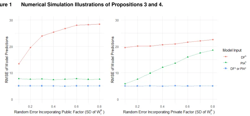
Figure 1 shows the results from numerical simulations (see Appendix B for details). The left panel cor-responds to Proposition 3. It varies the standard deviation of the public-factor random weight, holding constant the standard deviation of the private-factor random weight. Observe that the DF-PIA gap increases with the variability in the public-factor weight because the RMSE associated with Model-PIAb
Figure 1 Numerical Simulation Illustrations of Propositions 3 and 4.
Random Error Incorporating Private Factors. We now turn to examining the effect of random error on the DF-PIA gap when incorporating private factors. We proceed as above, by considering two cases that are identical except for the degree of variability inWb
i fori∈ I.
PROPOSITION4. The DF-PIA gap is smaller whenWfibis used in (5), fori∈ I, instead ofWib.
In contrast to Proposition 3, Proposition 4 shows that adding variability to how people incorporate private factors reduces the DF-PIA gap. Both Model-PIAband Model-DFblose accuracy as we add variability to
Wb
i, i∈ I. However, the loss is more dramatic for Model-PIA
b. PIA’s advantage of more directly eliciting the private information decreases as the random error incorporating private information increases.
The right panel of Figure 1 is the corresponding figure for Proposition 4. Observe that the DF-PIA gap decreases in the standard deviation of the private-factor random error term because while random error incorporating the private factor increases the RMSE under both Model-DFband Model-PIAb, the increase is steeper in the latter.
Summary and Hypothesis. Proposition 3 shows that the DF-PIA gap increases in the random error incor-porating public factors. Proposition 4 shows that the DF-PIA gap decreases in the random error incorpo-rating private factors. Combined, they imply that the DF-PIA will be greater when adding random error incorporating public information than when adding the same amount of random error incorporating private information. Based on these results, we formulate our second hypothesis:
Hypothesis 2 The location of random error moderates the DF-PIA gap. Specifically,
(a) Inducing greater random error incorporating public information increases the DF-PIA gap.
(c) Random error incorporating public information increases the DF-PIA gap more than random error
incorporating private information.
3.
Experiment 1: Elicitation via DF versus PIA
Experiment 1 is a simple direct test of Hypothesis 1. 3.1. Experimental Design
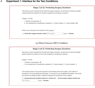
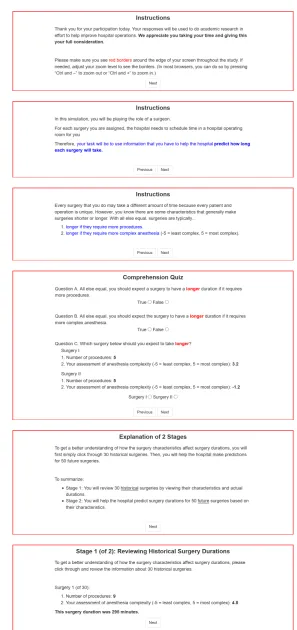
3.1.1. Task. Participants first reviewed30historical surgeries, each with information about the number of procedures, the anesthesia complexity score, and the resulting surgery duration. They then completed50 rounds of surgery duration prediction. In each round, they were shown a new surgery’s number of proce-dures and anesthesia complexity score. Then, they were asked a question about predicting its duration.
3.1.2. Conditions. Subjects were randomly assigned to one of two conditions: direct forecast (“DF”) or private information adjustment (“PIA”). The only difference between these two conditions is that in each of the 50 rounds, DF participants answered the question “What is your forecast for the duration of this surgery? I think this surgery duration will be minutes.”, whereas PIA participants answered the question “The hospital system only has the first piece of information about this surgery—the number of procedures. You have additional information. To account for your additional information, how would you advise the hospital system to adjust its forecast for the duration of this surgery? I would advise the hospital system to increase/decrease (choose one) its forecasted surgery duration by minutes.” See Appendix, Figure E.1 for screenshots.
3.1.3. Simulating Surgery Duration. We used the following equation to simulate surgery duration: Ys= 60 + 20XsP+ 10X
I
s+s. Here,Ysis the duration of surgerys;XsPdenotes the number of procedures, an integer-valued public factor that has a uniform distribution between1and10, inclusive; andXI
s denotes the anesthesia complexity score, a private factor that has a uniform distribution between−5and5. Finally, sfollows a normal distribution with mean0and standard deviation5. All participants observed the same30 simulated historical surgeries. However, each participant observed a unique sequence of randomly generated surgeries for their50prediction rounds.
3.1.5. Pre-registration. For all experiments, we set our target sample sizes, exclusion criteria, and analysis plans a priori. We pre-registered to exclude participants who (1) did not complete the experiment or (2) put the same answer more than 90% of the time. We also pre-registered our dependent variable and analyses. We calibrate prediction algorithms using data from the participants’ training set (first 35 rounds) and then use the algorithms to generate predictions on the test set (last 15 rounds). Our performance criterion is the RMSE of the predictions generated on the test set. The full pre-registration document for Experiment 1 is available athttps://aspredicted.org/blind.php?x=3e427n.
3.2. Results
3.2.1. Participant and Response Summary Statistics. Undergraduate and graduate students at a large research university in the US were invited to participate through a behavioral laboratory subject pool recruit-ment system. Each participant received a $10 electronic gift card for completing the online study.
A total of 120 students participated. Following our exclusion criteria, we removed 8 participants who did not complete the experiment, leaving 112 for analysis (56 in each condition). Among the 112 participants, 75% were female, 88% were 18 to 24 years old, and 12% were 25 to 34 years old. The average of mean response to the question was152.6minutes (SD30.8) in the DF condition and12.1minutes (SD23.7) in the PIA condition.
3.2.2. Algorithm Calibration and Prediction Accuracy Calculation. For each condition, we used the number of procedures, actual surgery duration, and participant response from all participants’ first35rounds to calibrate prediction algorithms for surgery duration. The pre-registered linear regression model included participant dummies, number of procedures interacted with participant dummies, and participant response interacted with participant dummies. Table E.1 in the Appendix summarizes the prediction algorithms cali-brated for each condition. We used the calicali-brated prediction algorithms to generate the predictions,Yˆs, for each surgerysin the last15rounds for each participant. We then computedRMSE=
q 1 15
P15
s=1(Ys−Yˆs) 2
for each participant.
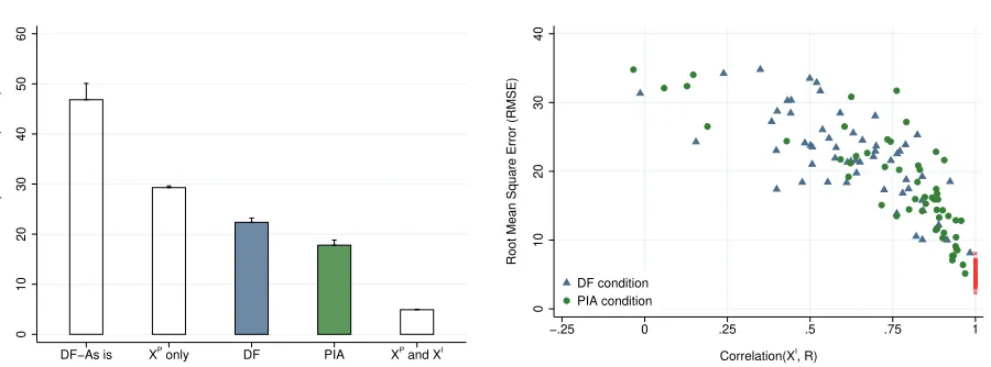
3.2.3. Testing Hypothesis 1. The average RMSE (averaged across all participants) was22.4(SD6.3) in the DF condition and 17.8 (SD 7.6) in the PIA condition; see Figure 2(a). This difference of 4.6 is significant (p= 0.0008) and represents a21%decrease. This result supports Hypothesis 1.
Figure 2 Experiment 1: Performance Comparison.
0
10
20
30
40
50
60
Root Mean Square Error (RMSE)
DF−As is XP
only DF PIA XP
and XI
(a) RMSE comparison. Means and standard errors are shown.
XP
is the public factor, andXI
is the private factor.
0
10
20
30
40
Root Mean Square Error (RMSE)
−.25 0 .25 .5 .75 1
Correlation(XI
, R) DF condition
PIA condition
(b) Correlation(XI,R) versus RMSE. Each dot is one
partici-pant.Ris defined as the residual of response after regressing it
onXP. Red x marks show the performance of the “XPandXI”
model.
“XP only” corresponds to using only the public information in the algorithm, without the use of any participant responses. Across the112participants, such an algorithm leads to an average RMSE of 29.3 (SD3.5)—an improvement over “DF-As is” even though participants had access to the private information in addition to the public information. However, it is worse than the average RMSE of both the DF condition (p <0.0001) and the PIA condition (p <0.0001). In other words, participant responses added predictive value in the experiment.
Lastly, “XPandXI” corresponds to allowing prediction algorithms to directly observe the private infor-mationXI and include it in prediction algorithms. In this experiment, it is equivalent to “consistent fore-casters” and is a benchmark for the best performance possible. This algorithm results in an average RMSE across the 112 participants of4.9(SD1.1).
3.2.5. Mechanistic Evidence. The theorized mechanism driving Hypothesis 1 is that PIA responses help the algorithm account for the private information better than the responses from the DF condition. To examine this mechanism, we calculate the correlation of the PIA responses withXI and compare them with the correlation of the DF responses withXI.
and PIA conditions. In contrast, we find that it is less than1in both conditions. However, it is significantly higher in the PIA condition than in the DF condition (0.76versus0.62,p= 0.0008). In other words, PIA responses provide better information aboutXI than DF responses.
Figure 2(b) illustrates the predictive accuracy versus the correlation value above for each participant. As expected, higher correlation betweenXI andRleads to better prediction performance. There are more participants with high correlation in the PIA condition than in the DF condition, which contributes to the better performance of the PIA condition overall. The red “x” marks indicate the hypothetical perfectly-consistent benchmark, with no random error for each participant, which yields perfect correlation for both DF and PIA conditions. The deviation of the PIA and DF dots from the red marks illustrates the effect of human random error in participant responses.
3.3. MTurk Replication
We replicated the same experiment with MTurk workers. Seehttps://aspredicted.org/blind. php?x=yv2vs7 for the pre-registration document. While overall, the predictions from the experiment with MTurk workers were less accurate, the between-condition results replicated, providing evidence of robustness across different populations. Appendix C provides details on the replication as well as a com-parison between the performances of university students and MTurk workers.
3.4. Discussion
Consistent with Hypothesis 1, Experiment 1 provides evidence that eliciting the PIA information instead of DF leads to better prediction algorithm performance. After the effect of public factor is taken out, participant responses are more correlated with the private factor. This tighter relationship helps prediction algorithms to incorporate private information, leading to better predictive performance. These results were replicated across university students and MTurk workers.
4.
Experiment 2: Manipulating Information Complexity of Public versus Private
Factors
Experiment 2 was designed to test Hypothesis 2, namely how the DF-PIA gap established in Experiment 1 is moderated by random error in incorporating public versus private factors. In addition, it provides a replication test of Hypothesis 1 using different surgery duration equations.
4.1. Experimental Design
random error, we automatically pre-aggregated multiple factors into a single representative factor for the participant.
Specifically, in the Baselinecase, we pre-aggregated information so that there was only one public and one private factor, as in Experiment 1. However, we required that participants account for two public factors in thePublic Info Complexcase or two private factors in thePrivate Info Complexcase. Thus, the experiment had a2(DF, PIA) by3(Baseline,Public Info Complex,Private Info Complex) between-subject experimental design.
The equations below show the underlying model we used for all conditions and the pre-aggregations we constructed to manipulate complexity by condition:
Ys = 150 + 10X P1
s + 10X P2
s + 10X I1
s + 10X I2
s +s (Underlying Model) = 150 + 10XsP1+ 10X
P2
s + (50 + 20X I
s) +s (Public Info Complex) = 150 + (50 + 20XP
s) + 10X I1
s + 10X I2
s +s (Private Info Complex) = 150 + (50 + 20XsP) + (50 + 20X
I
s) +s (Baseline). Here, XP1
s andX P2
s represent the two public factors. In the experimental task, they are the “procedure set-up requirements” and the “procedure complexity score,” respectively. Symmetrically,XI1
s andX I2
s rep-resent the two private factors. In the experimental task, they are the “anesthesia set-up requirements” and the “anesthesia complexity score,” respectively. The random generation process for public and private fac-tors was symmetric. For every surgerys,XP1
s andX I1
s were uniform random integers between0and10, inclusive.XP2
s andX I2
s were uniform random numbers between−5and5(rounded to the nearest tenth). We setXP
s = (X P1
s −5)/2 +X P2
s /2andX I s = (X
I1
s −5)/2 +X I2
s /2, which establishes the above equal-ities. In the experimental task, they are a generic “procedure score” and “anesthesia score,” respectively. See Appendix, Figure E.3 for screenshots. The pre-registration document for Experiment 2 is available at https://aspredicted.org/blind.php?x=9uq8dw.
4.2. Results
and the average response in each condition. We developed prediction algorithms in the same way as in Experiment 1 (see§3.2.2). Table E.2 in the Appendix summarizes the prediction algorithms.
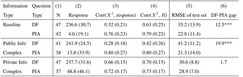
Table 1 Experiment 2: Summary of Experiment Results.
Information Question (1) (2) (3) (4) (5) (6)
Type Type N Response Corr(XI, response) Corr(XI,R) RMSE of test set DF-PIA gap
Baseline DF 47 236.6 (30.7) 0.52 (0.21) 0.63 (0.25) 35.2 (13.9) 12.5***
PIA 42 4.0 (19.1) 0.76 (0.23) 0.79 (0.22) 22.8 (11.4)
Public Info DF 41 241.9 (24.5) 0.28 (0.18) 0.42 (0.26) 41.2 (11.2) 19.9***
Complex PIA 38 13.8 (33.9) 0.80 (0.27) 0.80 (0.27) 21.3 (14.0)
Private Info DF 47 237.7 (31.6) 0.66 (0.15) 0.70 (0.15) 30.6 (8.8) 1.7
Complex PIA 37 48.8 (46.1) 0.72 (0.17) 0.73 (0.17) 28.9 (7.0)
Note.Means and standard deviations (in parentheses) are shown.XPis the public factor, andXIis the private factor. In column (4),Ris defined as the residual of response after regressing it onXP. In column (6), DF-PIA gap is defined as the difference between the mean RMSEs of DF and PIA conditions. Column (6) also shows DF-PIA gap’s statistical significance from a two-sample t-test for difference of means. *p <0.05, **p <0.01, ***p <0.001.
4.2.2. Robustness of Hypothesis 1. Columns (5) and (6) of Table 1 summarize the prediction perfor-mance in each of the six conditions. Consistent with Hypothesis 1, the average RMSE of all PIA participants was 32%lower than the average RMSE of all DF participants (35.4versus24.2, p <0.0001). As shown in column (6) of Table 1, the DF-PIA gap was statistically significant at the 5%level in two of the three information conditions. In§3.2.5, we found that better performance is associated with higher correlation between participant response andXI after the effect ofXP in the responses is taken out. Columns (3) and (4) of Table 1 provide the average correlation betweenXIand response and the average correlation between XI andR, defined as the residual of response after regressing it onXP. As expected, the correlations are higher in the PIA conditions than in the DF conditions, which again provides mechanistic evidence for Hypothesis 1.
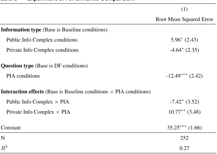
4.2.3. Testing Hypothesis 2. Hypothesis 2(a) predicts the DF-PIA gap to be greater under public-information-complex conditions than under baseline conditions. Consistent with this hypothesis, the gap was 19.9 under the public-information-complex conditions and 12.5 under the baseline conditions. This difference of7.4was statistically significant (p= 0.036; see Table 2).
Hypothesis 2(c) predicts the DF-PIA gap to be greater under public-information-complex conditions than under private-information-complex conditions. Consistent with this hypothesis, the gap was 19.9 under public-information-complex conditions and1.7under private-information-complex conditions. This differ-ence of18.2was statistically significant (p <0.001; see Table 2). These findings provide evidence that the benefit of PIA over DF is greater when public information is complex than when private information is complex.
One unpredicted pattern is that the RMSE in DF is smaller under the private-information-complex con-dition than under the baseline concon-dition (30.6versus35.2,p <= 0.056). A plausible explanation is that, in addition to inducing more random error, splitting the private information into two factors causes participants to weight the private information more in general (see Fox and Clemen (2005)).
Table 2 Experiment 2: Performance Comparison.
(1)
Root Mean Squared Error
Information type(Base is Baseline conditions)
Public Info Complex conditions 5.96∗(2.43)
Private Info Complex conditions -4.64∗(2.35)
Question type(Base is DF conditions)
PIA conditions -12.49∗∗∗(2.42)
Interaction effects(Base is Baseline conditions×PIA conditions)
Public Info Complex×PIA -7.42∗(3.52)
Private Info Complex×PIA 10.77∗∗(3.48)
Constant 35.25∗∗∗(1.66)
N 252
R2
0.27
Note.Column (1) is a linear regression model with RMSE as the dependent variable. +p <0.1, *p <0.05, **p <0.01, ***p <0.001.
4.3. Discussion
5.
General Discussion
5.1. SummaryOur theoretical and experimental results suggest that in some situations, there is an opportunity to substan-tially improve the way prediction algorithms incorporate human judgment by applying a new PIA elicitation method, instead of the traditional method of DF. Under DF, humans contribute random error as they account for public information that the algorithm can already access. This random error hinders the algorithm’s ability to infer the humans’ private information. PIA avoids this hindrance by asking more directly about the private information.
5.2. What Is Private Information and Why Does It Exist?
Pragmatically speaking, private information is any predictive information the human observes that the algo-rithm does not use. Because private information is context specific, rather than attempting to discuss exactly what it is, we find it constructive to discuss reasons why humans may have information that the algorithm does not use (i.e., why private information exists). We discuss these reasons in the context of our motivating example of predicting surgery durations: see Ibrahim and Kim (2019). At this hospital, the public informa-tion is the patient’s electronic medical record as well as answers to specific quesinforma-tions from a standardized booking slip for surgery. All other predictive information the surgeon has is private.
5.2.1. Identification Challenges. Some theoretically easy-to-input information may be private simply because the system fails to request it. In our experiments, private information is easy to identify because the researcher knows all the data that exist in the environment and what data the human can access that the algorithm cannot. In practice, such an exercise is more difficult because if information is kept private from the algorithm, it may also be kept from the system designer. In other words, you cannot ask for what you do not know exists. For example, a surgeon may need special anesthesia equipment that requires additional set-up time, but there may be no place to indicate this information on the booking slip because the system designer was unaware of this special equipment.
5.2.3. Codification Challenges. Despite advancements in “big data,” it often remains impractical to input and store certain types or large quantities of predictive information into an organization’s system. For example, one study reports that experienced doctors use nearly two million pieces of information to treat their patients (Pauker et al. 1976). While some of the two million pieces of information may be explicit knowledge—knowledge that can be easily articulated, codified, stored, and accessed—they are likely to be tacit knowledge, or knowledge that is difficult transfer, such as intuitive judgment; see Cowan et al. (2000) for a detailed discussion. As a result, inputting this information into the system will be costly and time consuming (Pollack et al. 2014), if not impossible.
5.2.4. Insufficient Training Data. Even if information has been inputted into the system, it may remain unused by the prediction algorithm due to a lack of sufficient historical data for training. Macario (2006) reports that 50% of surgeries have less than five previous cases with the same procedure and same surgeon during the preceding year. Zhou and Dexter (1998) report that only 32% of their surgeries had two or more previous cases with the same procedure and same surgeon. Ibrahim and Kim (2019) remove about 60% of the surgeries from their data collected over three years to keep only the surgeries that had 30 or more cases with the same procedure and same surgeon. The fact that each specialty, or even each procedure, has its own meaningful variables that are specific to the specialty or the procedure exacerbates the problem (Hosseini et al. 2015). Thus, the algorithm designer may intentionally choose to leave certain information as “private” because of lack of training data to make it useful.
5.3. What Should System Designers Do?
5.3.1. Consider Eliciting Human Input Even If Human Forecasts Are Inaccurate. Our study was motivated by a hospital administrator who, concerned with poor human forecasting performance, was con-sidering using algorithms and fully eliminating surgeons from the surgery duration forecast process. Our results highlight the fact that even when human forecasts are significantly worse than algorithms head-to-head, system designers can potentially significantly boost the algorithms’ performance by seeking human input. Thus, when implementing prediction algorithms, system designers should check to see whether human judgment can boost algorithm performance before fully replacing humans.
5.3.3. Identify and Convert Private Information into Public Information. The results of this paper suggest that PIA mitigates the undesirable impact of human random error relative to DF, but not completely. Directly converting private information to public information will be superior to eliciting private information from humans via PIA (e.g., see Figure 2) once enough training data have been collected. Thus, in addition to eliciting the PIA, we suggest attempting to learn what the underlying private information is behind humans’ answers and altering the system to collect or directly elicit it moving forward. While it is unlikely that one will be able to fully eliminate private information in this manner, in some contexts, one may be able to eliminate enough private information to render the improvement due to PIA or DF negligible.
5.3.4. Experiment with and Revise the PIA Elicitation Format. Because the type of private informa-tion is context specific, the best way to write the PIA quesinforma-tion is also likely to be context specific. Therefore, we suggest experimenting with and periodically revising how to write the PIA question. In Appendix D, we have made some limited progress on this issue via an experiment. We found that changing the format of the PIA question to make it easier for the human to translate from the domain of the private information to the domain of the question can enhance PIA’s performance. For example, on the one hand, if the private information is a relative assessment of complexity, then structure the PIA question as an assessment relative to an average patient with the same public information. On the other hand, if the private information is a delay in minutes, then format the PIA question to be in minutes.
5.4. How Can Future Research Help Improve (or Disprove) This PIA Idea?
One limitation of our laboratory study approach is that it does not directly address the question of whether PIA will outperform DF in practice. Certainly, field experiments or even more realistic laboratory experi-ments can help address this question. Nevertheless, our initial studies suggest that more investigation into how best to write the PIA question may be beneficial before one can confidently implement it and assess its performance relative to DF. How should one decide whether to make the PIA question in a relative domain (e.g., relative to an average case) or an absolute domain (e.g., in dollars)? What is the best way to describe public information in specific practical contexts? Should one decompose the PIA into multiple parts based on known categories of private information? Does showing the algorithm’s forecast before humans provide their PIA help or hurt? Are there algorithm aversion or incentive issues that need to be addressed before implementation?
model of random error that does not capture detail in how humans turn cues into predictions, where exactly the random error occurs, or how the format of the PIA question might matter. Another potentially fruitful direction is to incorporate further psychologically descriptive detail into a behavioral model of prediction.
In conclusion, field work, laboratory experiments, and behavioral models are all important for enhancing the understanding and use of PIA questions. It is our hope that by defining the PIA idea and documenting its potential improvement experimentally, we stimulate research that drives improvement in practice.
References
Alexander Jr JC (1995) Refining the degree of earnings surprise: A comparison of statistical and analysts’ forecasts.
Financial Review30(3):469–506.
Arvan M, Fahimnia B, Reisi M, Siemsen E (2019) Integrating human judgement into quantitative forecasting methods:
A review.Omega86:237–252.
Blattberg RC, Hoch SJ (1990) Database models and managerial intuition: 50% model+ 50% manager.Management
Science36(8):887–899.
Campbell D, Frei F (2011) Market heterogeneity and local capacity decisions in services.Manufacturing & Service
Operations Management13(1):2–19.
Carbone R, Andersen A, Corriveau Y, Corson PP (1983) Comparing for different time series methods the value of
technical expertise individualized analysis, and judgmental adjustment.Management Science29(5):559–566.
Childers CP, Maggard-Gibbons M (2018) Understanding costs of care in the operating room. JAMA Surgery
153(4):e176233–e176233.
Cowan R, David PA, Foray D (2000) The explicit economics of knowledge codification and tacitness.Industrial and
Corporate Change9(2):211–253.
Davis AM, Katok E, Kwasnica AM (2014) Should sellers prefer auctions? A laboratory comparison of auctions and
sequential mechanisms.Management Science60(4):990–1008.
Fildes R, Goodwin P, Lawrence M, Nikolopoulos K (2009) Effective forecasting and judgmental adjustments: An
empirical evaluation and strategies for improvement in supply-chain planning.International journal of
forecast-ing25(1):3–23.
Fox CR, Clemen RT (2005) Subjective probability assessment in decision analysis: Partition dependence and bias
toward the ignorance prior.Management Science51(9):1417–1432.
Goodwin P (2000) Correct or combine? Mechanically integrating judgmental forecasts with statistical methods.
Inter-national Journal of Forecasting16(2):261–275.
Hendriks A (2012) SoPHIE - Software platform for human interaction experiments. Working paper, University of
Osnabrueck.
Herzog SM, Hertwig R (2009) The wisdom of many in one mind: Improving individual judgments with dialectical
Ho TH, Zhang J (2008) Designing pricing contracts for boundedly rational customers: Does the framing of the fixed
fee matter?Management Science54(4):686–700.
Hosseini N, Sir MY, Jankowski C, Pasupathy KS (2015) Surgical duration estimation via data mining and predictive
modeling: a case study.AMIA Annual Symposium Proceedings, volume 2015, 640 (American Medical
Informat-ics Association).
Huang T, Allon G, Bassamboo A (2013) Bounded rationality in service systems.Manufacturing & Service Operations
Management15(2):263–279.
Ibrahim R, Kim SH (2019) Is expert input valuable? The case of predicting surgery duration.Seoul Journal of Business
25(2).
Kahneman D, Rosenfield A, Gandhi L, Blaser T (2016) Noise: How to overcome the high, hidden cost of inconsistent
decision making.Harvard Business Review36–43.
Kesavan S, Kushwaha T (2020) Field experiment on the profit implications of merchants’ discretionary power to
override data-driven decision-making tools.Available at SSRN 3619085.
Kim SH, Chan CW, Olivares M, Escobar G (2015) ICU admission control: An empirical study of capacity allocation
and its implication for patient outcomes.Management Science61(1):19–38.
Kremer M, Siemsen E, Thomas DJ (2016) The sum and its parts: Judgmental hierarchical forecasting.Management
Science62(9):2745–2764.
Lawrence M, Goodwin P, O’Connor M, ¨Onkal D (2006) Judgmental forecasting: A review of progress over the last 25
years.International Journal of forecasting22(3):493–518.
Lawrence M, O’Connor M, Edmundson B (2000) A field study of sales forecasting accuracy and processes.European
Journal of Operational Research122(1):151–160.
Macario A (2006) Are your hospital operating rooms “efficient”? A scoring system with eight performance indicators.
Anesthesiology: The Journal of the American Society of Anesthesiologists105(2):237–240.
Mannes AE, Larrick RP, Soll JB (2012) The social psychology of the wisdom of crowds. Krueger JI, ed.,Frontiers of
social psychology. Social judgment and decision making, 227–242 (Psychology Press).
Osadchiy N, Gaur V, Seshadri S (2013) Sales forecasting with financial indicators and experts’ input.Production and
Operations Management22(5):1056–1076.
Palley AB, Soll JB (2019) Extracting the wisdom of crowds when information is shared. Management Science
65(5):2291–2309.
Pauker SG, Gorry GA, Kassirer JP, Schwartz WB (1976) Towards the simulation of clinical cognition: taking a present
illness by computer.The American Journal of Medicine60(7):981–996.
Phillips R, S¸ims¸ek AS, Van Ryzin G (2015) The effectiveness of field price discretion: Empirical evidence from auto
Pollack AH, Tweedy CG, Blondon K, Pratt W (2014) Knowledge crystallization and clinical priorities: evaluating how
physicians collect and synthesize patient-related data.AMIA Annual Symposium Proceedings, volume 2014,
1874 (American Medical Informatics Association).
Rothschild M, Stiglitz JE (1970) Increasing risk: I. A definition.Journal of Economic Theory2(3):225–243.
Su X (2008) Bounded rationality in newsvendor models. Manufacturing & Service Operations Management
10(4):566–589.
Surowiecki J (2005)The wisdom of crowds(Anchor).
Tong J, Feiler D (2017) A behavioral model of forecasting: Naive statistics on mental samples.Management Science
63(11):3609–3627, URLhttp://dx.doi.org/10.1287/mnsc.2016.2537.
Vul E, Pashler H (2008) Measuring the crowd within: Probabilistic representations within individuals.Psychological
Science19(7):645–647.
Zhou J, Dexter F (1998) Method to assist in the scheduling of add-on surgical cases-upper prediction bounds for
sur-gical case durations based on the log-normal distribution.Anesthesiology: The Journal of the American Society
Appendix A: Proofs of Propositions
A.1. Proof of Proposition 1
Proof. To find the best fitting linear model of Y givenXi for i∈ P andDF
∗, we need to solve the following
optimization problem:
min α0,(αi)i∈P,βDF∗
E[(Y −α0− X
i∈P
αiXi−βDF∗DF∗)2]. (8)
Using the definition ofDF∗in (2), (8) is equivalent to
min α0,(αi)i∈P,βDF∗
E[(Y−(α0+βDF∗v∗)−
X
i∈P
(αi+βDF∗wi∗)Xi−
X
i∈I
βDF∗wi∗Xi)2]. (9)
Similarly, to find the best fitting linear model ofY givenXifori∈ P andPIA∗, we need to solve the following
optimization problem:
min γ0,(γi)i∈P,βPIA∗E
[(Y−γ0− X
i∈P
γiXi−βPIA∗PIA∗)2]. (10)
Using the definition ofPIA∗in (2), (10) is equivalent to
min γ0,(γi)i∈P,βPIA∗E
[(Y −γ0− X
i∈P
γiXi−
X
i∈I
βPIA∗w∗
iXi)
2]. (11)
We note that by letting
α0+βDF∗v∗=γ0, αi+βDF∗w∗
i =γi fori∈ P, and βDF∗=βP IA∗,
there is a one-to-one correspondence between all feasible solutions for problems (9) and (11). That is, the two
opti-mization problems are equivalent, andMDF∗andMPIA∗must yield the same predictions.
A.2. Proof of Proposition 2
Proof. To find the best fitting linear model of Y givenXi for i∈ P andDFb, we need to solve the following
optimization problem:
min α0,(αi)i∈P,βDF b
E[(Y −(α0+βDFbvb)−
X
i∈P
(αi+βDFbWib)Xi−
X
i∈I
βDFbWibXi)2] (12)
Similarly, to find the best fitting linear model ofY givenXi fori∈ P andPIAb, we need to solve the following
optimization problem:
min γ0,(γi)i∈P,βP IAb
E[(Y−γ0− X
i∈P
γiXi−
X
i∈I
βP IAbWibXi)2]. (13)
We now show that for any feasible solution ( ¯α0,( ¯αi)i∈P,β¯DFb) for problem (12), we can construct a feasible
solution(¯γ0,(¯γi)i∈P,β¯P IAb)for (13) that yields astrictlysmaller objective value by letting:
¯
γ0= ¯α0+ ¯βDFbvb, ¯γi= ¯αi+ ¯βDFbw¯bi fori∈ P, and β¯P IAb= ¯βDFb, (14)
where we recall thatE[Wib] = ¯w b i.
Note that the objective value for problem (12) with( ¯α0,( ¯αi)i∈P,β¯DFb)is:
E[(Y −( ¯α0+ ¯βDFbvb)−
X
i∈P
( ¯αi+ ¯βDFbWib)Xi−
X
i∈I ¯
We defineV andUas follows:
V =Y−γ0¯ −X
i∈P ¯ γiXi−
X
i∈I ¯
βP IAbWibXi and U=
X
i∈P
( ¯αi+ ¯βDFbWib)Xi−
X
i∈P
( ¯αi+ ¯βDFbw¯bi)Xi.
Then, utilizing (14) and the definitions ofV andU, (15) can be written as follows:
E
Y −( ¯α0+ ¯βDFbvb)−
X
i∈P
( ¯αi+ ¯βDFbWib)Xi−
X
i∈I ¯
βDFbWibXi+
X
i∈P
( ¯αi+ ¯βDFbw¯bi)Xi−
X
i∈P
( ¯αi+ ¯βDFbw¯ib)Xi
!2
=E
(Y −¯γ0−
X
i∈P ¯ γiXi−
X
i∈I ¯
βP IAbWibXi)−(
X
i∈P
( ¯αi+ ¯βDFbWib)Xi+
X
i∈P
( ¯αi−β¯DFbw¯bi)Xi)
!2
=E[(V −U)2]
=E[V2] +
E[U2]−2E[V U]
=E[V2] +E[U2]
>E[V2].
Note that in the fifth equation we use:
E[V U] =E[E[V U|Xi∈ P]]
=E[E[V|Xi∈ P]E[U|Xi∈ P]]
= 0,
sinceE[U|Xi, i∈ P] = 0andUandV are conditionally independent onXi∈ P. Also note thatE[U2] =Var[U]>0
since Var[Wb i]>0.
Notice thatE[V2]is the objective value for problem (13) with(¯γ0,(¯γi)i∈P∪I,β¯P IAb). The reasoning above holds
for any feasible solution for problem (12). In particular, it holds for the optimal solution at the optimal value. Thus,
the mean squared error (MSE) for predictions under Model-DFbis strictly larger than that under Model-PIAb.
A.3. Proof of Proposition 3
Proof. Recall that we definedWfibto be a mean preserving spread ofW b
i. By the definition of mean preserving spread
(Rothschild and Stiglitz 1970), we can letWfib=Wib+ Γi, where we assumeE[Γi] = 0and Var[Γi]>0.
Note that whenfWibis used in (5) fori∈ P instead ofWib, Model-PIAb does not change because PIA responses
are unaffected by the random error incorporating public factors. Thus, we only need to compare the performance of
Model-DFbwhen
f Wb
i is used in (5) fori∈ PversusW b i.
To find the best fitting linear model ofY givenXi fori∈ P andDFb withWfib fori∈ P, we need to solve the
following optimization problem:
min
e
α0,(eαi)i∈P,βeDF b
E[(Y −(αe0+βeDFbv
b)−X
i∈P
(αei+βeDFb(Wib+ Γi))Xi−
X
i∈I
e
βDFbWibXi)2] (16)
Similarly, to find the best fitting linear model ofY givenXifori∈ PandDFbwithWibfori∈ P, we need to solve
the following optimization problem:
min α0,(αi)i∈P,βDF b
E[(Y−(α0+βDFbvb)−
X
i∈P
(αi+βDFb(Wib))Xi−
X
i∈I
We now show that for any feasible solution (αe0,(αei)i∈P,βeDFb) for problem (16), we can construct a feasible
solution(α0,(αi)i∈P, βDFb)for (17) that yields astrictlysmaller objective value by letting:
e
α0+βeDFbvb=α0+βDFbvb, αei=αi fori∈ P, and βeDFb=βDFb. (18)
LetV =Y−(α0+βDFbvb)−Pi∈P(αi+βDFbWib)Xi−
P
i∈IβDFbWibXi. Then, utilizing (18) and the definition
ofV, the objective value for problem (16) with(α0,e (αei)i∈P,βeDFb)can be written as follows:
E
Y−(αe0+βeDFbvb)−
X
i∈P
(αei+βeDFb(Wib+ Γi))Xi−
X
i∈I
e
βDFbWibXi
!2
=E
Y−(α0+βDFbvb)−
X
i∈P
(αi+βDFbWib)Xi−
X
i∈I
βDFbWibXi−
X
i∈P
βDFbΓiXi
!2
=E[(V−
X
i∈P
βDFbΓiXi)2]
=E[V2] +E[(
X
i∈P
βDFbΓiXi)2]−2E[V ·
X
i∈P
βDFbΓiXi]
>E[V2],
since
E[V·X i∈P
βDFbΓiXi] = E[E[V
X
i∈P
βDFbΓiXi
Xi∈ P]]
= 0,
because of conditional independence onXi, i∈ P, and the fact thatE[Γi] = 0. Note thatE[V2]is the objective value
for problem (17) with(α0,(αi)i∈P, βDFb).
A.4. Proof of Proposition 4
In the interest of algebraic tractability, we present here the proof for the case where there is one public factor and one
private factor only. It is straightforward to generalize the proof for cases with more than one public factor and one
private factor using the same approach.
Proof. We let X1 be a public factor and X2 be a private factor. By the definition of mean preserving spread
(Rothschild and Stiglitz 1970), we can letWfib=Wib+ Γi, where we assumeE[Γi] = 0and Var[Γi]>0.
We first define a general optimization problem that finds the best fitting linear model ofY givenX1and responses
(DF or PIA):
Z(γ, W) = min α0,α1,β
E
Y −(α0+γβvb)−(α1+γβW1b)X1−βW X2
2
. (19)
Here,α0 is the calibrated intercept,α1is the coefficient forX1, andβ is the coefficient for response (DF or PIA).
By choosingγandW appropriately, we can define the following four models for different combinations of using DF
versus PIA and usingWb
2 versusWf2b:
A=Z(1, Wb
2) = minα
0,α1,β
E
Y −(α0+βvb)−(α1+βW1b)X1−βW2bX2
2
,
B=Z(0, Wb
2) = min
α0,α1,β
E
Y −α0−α1X1−βW2bX2
2
C=Z(1,fW2b) = min
α0,α1,β
E
Y −(α0+βvb)−(α1+βW1b)X1−βWf2bX2
2
,
D=Z(0,fW2b) = min
α0,α1,β
E
Y −α0−α1X1−βWf2bX2
2
,
whereWf2b=W2b+ ΓandE[Γi] = 0and Var[Γi]>0. In general:
We assume that the actual surgery durationY is defined as follows:
Y =δ0+δ1X1+δ2X2+ε.
We can then show:
Z(γ, W) = min α0,α1,β
E
Y −(α0+γβvb)−(α1+γβW1b)X1−βW X2
2
= min α1,β
Var
Y−γβvb
−(α1+γβW1b)X1−βW X2
= min α1,βVar
Y−(α1+γβW1b)X1−βW X2
= min α1,β
Varε+ (δ1−α1−γβW1b)X1+ (δ2−βW)X2
= min λ1,β
Var
ε+ (λ1−γβW1b)X1+ (δ2−βW)X2
= min λ1,β
Var
ε+λ1X1−γβW1bX1+δ2X2−βW X2
= min λ1,β
Var[ε] +λ2
1Var[X1] +γ2β2Var[W1bX1] +δ22Var[X2] +β2Var[W X2]
−2λ1γβCov(X1, W1bX1)−2δ2βCov(X2, W X2)
=Var[ε] +δ22Var[X2]
+ min λ1,β
λ21Var[X1] +γ2β2Var[Wb 1X1] +β
2Var[W X2]−2λ1γβVar(X1)E[Wb
1]−2δ2βCov(X2, W X2)
=Var[ε] +δ22Var[X2]
+ min β min λ1
Var[X1]λ21−2γβVar(X1)E[W1b]λ1
+β2(γ2Var[Wb
1X1] + Var[W X2])−2δ2βCov(X2, W X2)
=Var[ε] +δ22Var[X2]
+ min β
γ2β2Var[Wb
1X1]−γ2β2E[W1b] 2Var[X
1] +β2Var[W X2]−2δ2βVar(X2)E[W]
=Var[ε] +δ22Var[X2] + min β
γ2Var[Wb
1X1]−γ2E[W1b] 2Var[X
1] + Var[W X2]
β2−2
δ2Var(X2)E[W]
β
=Var[ε] +δ22Var[X2]−
(δ2Var(X2)E[W])2 γ2Var[Wb
1X1]−γ2E[W1b]2Var[X1] + Var[W X2]
=Var[ε] +δ22Var[X2]−
(δ2Var(X2)E[W])2 γ2Var[Wb
1]E[X12] + Var[W X2] .
Note thatE[Wb
2] =E[Wf2b]. DenoteM≡(δ2Var[X2]E[W2b])2= (δ2Var[X2]E[Wf2b])2. Then, we obtain:
(A−B)−(C−D) =(− (δ2Var(X2)E[W
b 2])
2
Var[Wb
1]E[X12] + Var[W2bX2]
+(δ2Var(X2)E[W b 2])
2
Var[Wb 2X2]
)
−(− (δ2Var(X2)E[Wf
b 2])
2
Var[Wb
1]E[X12] + Var[Wf2bX2]
+(δ2Var(X2)E[Wf b 2])
2
Var[Wf2bX2] )
=(− M
Var[Wb
1]E[X12] + Var[W2bX2]
+ M
Var[Wb 2X2]
)
−(− M
Var[Wb
1]E[X12] + Var[Wf2bX2]
+ M
Var[fW2bX2] )
= MVar[W
b 1]E[X12] (Var[Wb
1]E[X12] + Var[W2bX2])(Var[W2bX2])
− MVar[W
b 1]E[X12]
(Var[Wb
1]E[X12] + Var[Wf2bX2])(Var[fW2bX2])
=MVar[Wb 1]E[X
2 1]
1 (Var[Wb
− 1
(Var[Wb
1]E[X12] + Var[Wf2bX2])(Var[Wf2bX2])
≥0,
where the last inequality follows fromVar[fW2bX2] = Var[(W2b+ Γ)X2] = Var[W2bX2] + Var[ΓX2]≥Var[W2bX2].
Appendix B: Numerical Simulation Details
To construct Figure 1, we programmed a numerical simulation in R (script available from the authors upon request).
As in Experiment 1 (see§3), we simulated true surgery durations according toYs= 60 + 20XsP+ 10X I
s+s, where XP
s are uniform random numbers between1and10(inclusive),X I
s are uniform random numbers between -5 and 5
(rounded to the tenths position), andsare normally distributed with mean0and standard deviation5.
We simulated the inconsistent forecaster’s coefficients,Wb
is in (5), by adding normally distributed random error
with mean0to the rational forecaster’s coefficients,w∗
is in (2). Specifically, to create the left figure, we varied the
standard deviation of the normally distributed random error added to the inconsistent forecaster’s coefficient for the
public factor, holding constant the standard deviation of the normally distributed random error added to the
inconsis-tent forecaster’s coefficient for the private factor at0.2. Similarly, for the right figure, we varied the standard deviation
of the normally distributed random error added to the inconsistent forecaster’s coefficient for the private factor,
hold-ing constant the standard deviation of the normally distributed random error added to the inconsistent forecaster’s
coefficient for the public factor at0.2.
For each point in the figure, the script executed the following steps:
1. Simulate10,000“actual” surgery durations.
2. Fit a linear model based on the simulated public and private factors. We used these coefficients to define thew∗ is
in (2) for a rational forecaster.
3. Calculate the rational forecaster’s DF and PIA values for each surgery based on thesew∗ is.
4. Simulate the inconsistent forecaster’s coefficientsWb
is in (5) for each surgery by adding normal random error
with mean0to thew∗ is.
5. Define the inconsistent forecaster’s DF and PIA for each surgery based on these randomWb is.
6. Split the dataset in half to define a train and test set.
7. Calibrate Model-DF∗, Model-PIA∗, Model-DFb, and Model-PIAb in (3), (4), (6), and (7), respectively, using
the train set data.
8. Predict surgery durations onto the test set using these calibrated models.
Appendix C: Replicating Experiment 1 with MTurk Workers
The experiment was identical to Experiment 1 except for the study population; we recruited MTurk workers instead
of university students. The pre-registration document for this experiment is available athttps://aspredicted.
org/blind.php?x=yv2vs7.
MTurk workers who were located in the US, had a Human Intelligence Task (HIT) approval rate of 99% or higher,
and had 100 or more HITs approved were qualified to participate in the experiment. Participants who completed the
experiment were paid $2 for participation. A total of 160 MTurk workers participated. Following the pre-registered
exclusion criteria, we removed 37 individuals who did not complete the experiment, leaving 123 participants for
analysis. Among the 123 participants, 47% were female and 9% were 18 to 24 years old; 43%, 25 to 34; 30%, 35 to
44; 11%, 45 to 54; and 7%, 55 or over.
Table C.1 provide a summary of experiment results and Table C.2 summarizes the prediction algorithms. The
aver-age RMSE was26.0in the DF condition and22.5in the PIA condition. The difference of3.5is significant (p= 0.0085)
and represents a 13% decrease. As in Experiment 1, the correlation between XI andR—defined as the residual
of participant response after regressing it onXP—was significantly higher in the PIA condition (0.61versus0.49,
p= 0.0191).
Table C.1 Replicating Experiment 1 with MTurk Workers: Summary of Experiment Results.
(1) (2) (3) (4) (5) (6)
Condition N Response Corr(XI, response) Corr(XI,R) RMSE of test set DF-PIA gap
Direct Forecast (DF) 68 154.0 (37.3) 0.29 (0.22) 0.49 (0.24) 26.0 (5.8) 3.5**
Private Information Adjustment (PIA) 55 20.2 (35.3) 0.57 (0.33) 0.61 (0.30) 22.5 (8.7)
Note.Means and standard deviations (in parenthesis) are shown.XPis public factor andXIis private factor. In column (4),Ris defined as the residual of response after regressing it onXP. In column (6), DF-PIA gap is defined as the difference between the mean RMSEs of DF and PIA. Column (6) also shows DF-PIA gap’s statistical significance from a two-sample t-test for difference of means. *p <0.05, **p <0.01, ***
p <0.001.
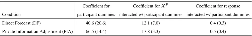
Table C.2 Replicating Experiment 1 with MTurk Workers: Prediction Algorithms for Each Condition. Coefficient for Coefficient forXP
Coefficient for response
Condition participant dummies interacted w/ participant dummies interacted w/ participant dummies
Direct Forecast (DF) 40.6 (20.6) 12.1 (7.0) 0.4 (0.3)
Private Information Adjustment (PIA) 66.5 (14.4) 17.8 (3.3) 0.5 (0.4)
Table C.3 provides detailed summary statistics comparing students and MTurk workers in Experiment 1 and this
experiment. In addition, Table C.4 provides a more detailed comparison of RMSE. Although students and MTurk
workers did not differ in their responses or in their time to provide the responses, the comparison results suggest that
students were significantly better at our task than MTurk workers. An important takeaway, however, is that the benefit
Table C.3 University Students versus MTurk Workers.
DF PIA
Student MTurk p-value Student MTurk p-value
N 56 68 56 55
Response 152.6 (30.8) 154.0 (37.3) 0.819 12.1 (23.7) 20.2 (35.3) 0.160
Corr(XI,response) 0.39 (0.20) 0.29 (0.22) 0.018 0.74 (0.26) 0.57 (0.33) 0.003
Corr(XI,R) 0.62 (0.20) 0.49 (0.24) 0.003 0.76 (0.24) 0.61 (0.30) 0.004
RMSE of test set 22.4 (6.3) 26.0 (5.8) 0.001 17.8 (7.6) 22.5 (8.7) 0.003
Average response time (seconds) 10.2 (6.4) 10.7 (8.3) 0.692 12.5 (9.3) 13.2 (7.5) 0.692
Note.Mean, standard deviation (in parentheses), andp-value from independent-samples t-test are reported.
Table C.4 RMSE Comparison of University Students versus MTurk Workers.
(1)
Root Mean Squared Error
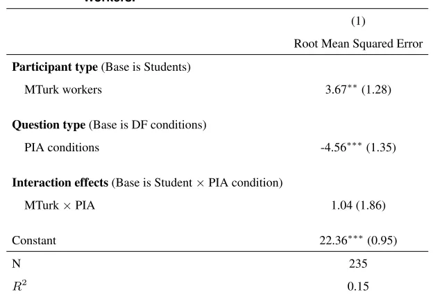
Participant type(Base is Students)
MTurk workers 3.67∗∗(1.28)
Question type(Base is DF conditions)
PIA conditions -4.56∗∗∗(1.35)
Interaction effects(Base is Student×PIA condition)
MTurk×PIA 1.04 (1.86)
Constant 22.36∗∗∗(0.95)
N 235
R2 0.15
Note.Columns (1) is a linear regression model with RMSE as the dependent variable. +p <
Appendix D: Changing the Format of the Private Information Adjustment (PIA) Question
Because we use human judgments asinputsto algorithms, responses need not be in the same domain as the ultimate
forecast (in our case, minutes). Any linear transformation of DF and PIA responses defined in (5) are equivalent from
the algorithm’s perspective. This observation is practically relevant because it broadens the range of possible formats
that the system designer can use to elicit the PIA. A designer may search this broader range of possibilities to try to
reduce human random error, lower the effort required, and enhance PIA’s performance.
We conduct an experiment to test whether Hypothesis 1 is robust even when the PIA question is formatted as a
non-numeric multiple choice question. We further conjecture that structuring the PIA question in a way that reduces
the cognition required to translate the private information into the domain requested can potentially reduce random
error incorporating the private information, leading to enhanced PIA performance.
D.1. Experimental Design
The experiment was similar to Experiment 1, but with the additional manipulation of a 5-point scale multiple-choice
question format for both DF and PIA. Thus, the experiment had a2answer types (numeric or multiple choice) by2
question types (DF or PIA) between-subject design.
Participants assigned to the Multiple choice-DF condition were asked: “I think this surgery duration will be: a) a lot
shorter than average, b) a little shorter than average, c) about average, d) a little longer than average, e) a lot longer than
average.” On the other hand, participants assigned to the Multiple choice-PIA condition were asked: “Of the above
two characteristics of this future surgery, the hospital system only knows about the number of procedures. Compared
to surgeries with the same number of procedures, I would advise the hospital system that this surgery duration will be:
a) a lot shorter than average, b) a little shorter than average, c) about average, d) a little longer than average, e) a lot
longer than average.”
We conjectured that even though the multiple-choice format can convey less precise information than the numeric
format, it may be cognitively easier (thereby reducing random error) for participants to translate the private information
(a score between -5 and 5) to this multiple choice format as opposed to attempt to convert to minutes in the numeric
format. The pre-registration document for the experiment is available athttps://aspredicted.org/blind.
php?x=mx2if3.1
D.2. Results
D.2.1. Participants, Participant Response, and Prediction Algorithms. The MTurk worker qualification and
payment settings were the same as in Experiment 2 (see§4.2.1). A total of 200 MTurk workers participated. Following
the pre-registered exclusion criteria, we removed 30 individuals who did not complete the experiment. Among the 170
remaining participants, 45% were female, 9% were 18 to 24 years old; 45%, 25 to 34; 30%, 35 to 44; 13%, 9 to 54;
and 6%, 55 or over. Columns (1) and (2) of Table D.1 provide the number of participants and the average response in
each condition.
1
Table D.1 Changing the Format of the PIA Question: Summary of Experiment Results.
Answer Question (1) (2) (3) (4) (5) (6)
Type Type N Response Corr(XI, response) Corr(XI,R) RMSE of test set DF-PIA gap
Numeric DF 46 159.9 (30.1) 0.30 (0.18) 0.52 (0.26) 28.4 (5.4) 5.0*
PIA 32 26.7 (29.2) 0.56 (0.35) 0.62 (0.33) 23.4 (11.6)
Multiple choice DF 44 11%, 15%, 24%, 28%, 21% 0.34 (0.27) 0.48 (0.31) 27.5 (6.2) 8.6**
PIA 48 17%, 15%, 21%, 28%, 19% 0.64 (0.37) 0.71 (0.35) 18.9 (12.5)
Note.Means and standard deviations (in parenthesis) are shown. For multiple choice conditions, the average percentage of each response is provided in the following order: ‘a lot shorter than average’; ‘a little shorter than average’; ‘about average’; ‘a little longer than average’; and ‘a lot longer than average.’ We coded ‘a lot shorter than average’ as 1, ‘a little shorter than average’ as 2, ‘about average’ as 3, ‘a little longer than average’ as 4, and ‘a lot longer than average’ as 5 for correlation computation and prediction algorithm development.XPis public factor andXIis private factor. In column (4),Ris defined as the residual of response after regressing it onXP. In column (6), DF-PIA gap is defined as the difference between the mean RMSEs of DF and PIA conditions. Column (6) also shows DF-PIA gap’s statistical significance from a two-sample t-test for difference of means. *p <0.05, **
p <0.01, ***p <0.001.
We developed prediction algorithms in the same way as Experiment 1 (see§3.2.2). As was pre-registered, we used
the first 20 rounds of each participant to develop prediction algorithms and the last 20 rounds to evaluate prediction
performance. Table D.2 summarizes the prediction algorithms.
Table D.2 Changing the Format of the PIA Question: Prediction Algorithms for Each Condition. Coefficient for Coefficient forXP Coefficient for response
Answer type Question type participant dummies interacted w/ participant dummies interacted w/ participant dummies
Numeric DF 27.8 (20.4) 8.7 (10.0) 0.6 (0.4)
PIA 67.2 (13.2) 16.9 (4.4) 0.7 (0.6)
Multiple choice DF 20.0 (35.8) 15.2 (5.9) 19.5 (18.3)
PIA 7.9 (32.8) 17.5 (5.4) 20.8 (15.9)
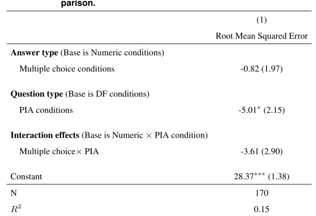
D.2.2. Performance Comparison. Columns (5) and (6) of Table D.1 summarize the prediction performance of
the four conditions. Consistent with Hypothesis 1, the results show robust support for the benefit of eliciting human
judgment via PIA over DF. The DF-PIA gap was5.0(p= 0.0121) in numeric conditions and8.6 (p= 0.0001) in
multiple-choice conditions. The DF-PIA gap was directionally larger under multiple choice, but the difference was
not statistically significant (p= 0.2152; see Table D.3). In addition, columns (3)-(4) of Table D.1 show the average
correlation betweenXI and the response and the average correlation betweenXI andR, respectively. The higher
correlation values betweenXIandRin PIA conditions show, once more, strong mechanism evidence for Hypothesis
1.
The average RMSEs in numeric versus multiple choice conditions were not statistically different within DF
con-ditions (28.4versus27.5,p= 0.5016). Within the PIA conditions, RMSEs were directionally better under multiple
choice versus numeric, although the difference was not statistically significant at the 5% level (23.4 versus 18.9,
p= 0.1138). The RMSEs in the best performing condition, Multiple choice-PIA, were significantly better than the