DOI: 10.1051/epjconf/201510401005
C
Owned by the authors, published by EDP Sciences, 2015
Neutron reflectivity
Fabrice Cousin and Alain Menelle
Laboratoire Léon Brillouin, CEA-CNRS, CEA-Saclay, 91191 Gif-sur-Yvette, France
Abstract.The specular neutron reflectivity is a technique enabling the measurement of neutron scattering length density profile perpendicular to the plane of a surface or an interface, and thereby the profile of chemical composition. The characteristic sizes that are probed range from around 5 Å up 5000 Å. It is a scattering technique that averages information on the entire surface and it is therefore not possible to obtain information within the plane of the interface. The specific properties of neutrons (possibility of tuning the contrast by isotopic substitution, sensitivity to magnetism, negligible absorption, low energy of the incident neutrons) makes it particularly interesting in the fields of soft matter, biophysics and magnetic thin films. This course is a basic introduction to the technique and does not address the magnetic reflectivity. It is composed of three parts describing respectively its principle and its formalism, the experimental aspects of the method (spectrometers, samples) and two examples related to the materials for energy.
Résumé.La réflectivité spéculaire des neutrons est une technique permettant de mesurer le profil de densité de longueur de diffusion de neutron, et ce faisant le profil de composition chimique, perpendiculairement à une surface ou une interface plane. Les tailles caractéristiques sondées sont de l’ordre de 5 Å à 5000 Å. C’est une technique de diffusion qui moyenne l’information sur l’ensemble de la surface et qui ne permet donc pas d’obtenir d’informations dans le plan de l’interface. Les propriétés spécifiques des neutrons (possibilité de moduler le contraste par substitution isotopique, sensibilité au magnétisme, absorption négligeable, faible énergie des neutrons incidents) la rendent particulièrement intéressante dans les domaines de l’étude de la matière molle, de la biophysique et des couches minces magnétiques. Ce cours est une simple introduction à la technique et ne traite pas la réflectivité magnétique. Il est composé de trois parties décrivant respectivement son principe et son formalisme, les aspects expérimentaux de la méthode (spectromètres, échantillons) et deux exemples en lien avec les matériaux pour l’énergie.
1. Introduction
Neutron reflectivity (NR) is a technique enabling to measure the thickness and the chemical composition of one or several thin layers at a surface or at interface. The typical order of magnitude of the thicknesses that can be measured experimentally lie in the range 5 Å–5000 Å. The principle is to measure the coefficient of reflection R of a neutron beam sent in grazing incidence on the surface that is to be studied. In this course, we will focus only on the specular reflectivity that provides only the profile of chemical composition perpendicular to the surface. This specular reflectivity corresponds to the reflection of neutrons making the same angleto the surface that the incident beam. Since it is a scattering technique,
Table 1. Coherent scattering length of some atoms and scattering length density of some molecules. PS refers to
polystyrene.
Coherent scattering length b (10−12cm)
1H D (2H) C O N Si Ni Ti
−0.374 0.667 0.665 0.580 0.936 0.415 1.03 −0.344
Scattering length density (Å−2)
H2O D2O PSH PSD SiO2 Si(crystal) Ni(crystal) Ti(crystal)
−0.56 10−6 6.38 10−6 1.41 10−6 6.5 10−6 3.41 10−6 2.07 10−6 9.4 10−6 −1.95 10−6
such a profile will be averaged on the whole surface and the technique and NR will not provide any information on the possible in-plane structure at the surface. It is thus usually very valuable to combine NR with a technique enabling such in-plane structure information, either a scattering method (GISAS, surface diffraction, off-specular measurements) or a microcopy (AFM, Brewster micrsocopy..).
The lower limit of thickness that can be measured is directly linked to the minimal reflectivity that can be experimentally obtained (Vide Infra). Given the actual brightness of the neutrons sources, such minimal reflectivity is of the order of 10−6 to 10−7 on samples of a few cm2. This is of the same order of what can be measured by X-Ray reflectivity, whose principle is similar to NR, on laboratory apparatus. Such minimal X-Ray reflectivity can be extended down to 10−10, id est one photon being reflected for 10 billions, on synchrotrons sources. X-rays measurement have thus to be preferred in many experimental cases. Neutrons have however some unique specific properties with respect to photons that enables some measurements that cannot be achieved with X-rays, essentially for the characterization of buried interfaces and for the study of materials containing hydrogen or for magnetic materials. Such specificities have made NR experiments very popular since the early 90’s.
The first of such specificities concerns the neutron-matter interaction that directly occurs between the neutron and the nuclei of atoms, and not with the electronic cloud, as for X-rays. This interaction has a very short range and is usually represented by the Fermi pseudo-potential punctual and centered on the atom. As a consequence, it differs from one isotope of a given atom to another. The amplitude of such interaction, id est the coherent scattering length, is tabulated and varies randomly from one atom to another along the periodic table of elements. The coherent scattering length can be either positive or negative, contrarily to the case of X-rays for which is always positive and proportional to the number of electrons. The values of some representative atoms are reported in Table1. It appears that the of hydrogen1H has an opposite sign and a very different value than the ones of all other atoms constitutive organic molecules (C,O,N..) and, last but not least, than the one from deuterium2H. This enables to achieve experiments on organic materials because the amplitude of the interaction of a given organic molecule with neutrons (averaged on all of its atoms), and therefore its neutron refraction index, is essentially dependent on its content on hydrogen atoms. In particular, the replacement of some hydrogen atoms of a molecule by deuterium atoms will strongly modify its refraction index without altering its physical properties. It opens the way to contrast variation experiments where some molecules are labeled by deuterium to create a neutron contrast in the system. It is also possible to continuously tune the neutron refractive index of a solvent in a complex system by mixing hydrogenated and deuterated solvents in order to match the one of a component, making it invisible from the neutron point of view. Such contrast variation experiments, which have been very successfully applied in soft matter in the field of surfactants and polymers (1), (2), (3) or in biophysics (4), have great potential for functional materials coated by organic thin layers such as solar cells.
As they bear a spin±1/2, the second important specificity of neutrons is their ability to interact
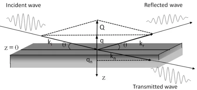
Figure 1. Reflection on an infinite planar surface.
The third important property of neutrons is their very weak absorption by matter (they do not interact with electric fields..) that can be neglected in general, except in cases when on probes materials containing one of the few atoms that have a huge neutron absorption cross-section (boron, gadolinium, lithium, ...). The neutron refractive indexes have thus no imaginary part, contrarily to its counterpart in in X-Ray reflectivity. It is then possible to study buried interfaces or to perform in situ experiments in various sample environments.
The fourth and last important characteristic of neutrons is their weak energy. After their thermalization at the wavelengths required for experiments, they have an energy of a few meV. The NR experiments are thus absolutely not destructive, which is of great importance in biology or for the expertise of industrial devices.
This course is divided in three parts. We will present in the first part the principle of NR by an approach where the spin of neutrons is not taken into account. This approach is no longer valid for magnetic systems (2). The formalism that treats correctly the magnetism can be found in (5). Besides, the off-specular aspects of reflectivity are not presented here. We will describe in the second part how it is possible to realize a NR experiment from practical point of view (description of spectrometers and of possible geometries of measurements, sample environments, accessibility to neutrons beams. . .). Finally two examples related with materials for energy will be presented in the third part.
2. Principle of neutron reflectivity
The formalism described in this part is a wave formalism very close to the one of light. Please remember that is it not applicable for magnetism and that the absorption of neutrons is not considered here.
2.1 Neutron-matter interaction and calculation of refractive index for neutrons
Let consider a neutrons beam reflecting on an infinite flat surface with an incident angle(see Fig.1). This surface is defined by the interface between the vacuum (n=1) and a media with a refraction index n. In vacuum, the modulus of the wave vector of an incident neutron of wavelength is defined by:
The energy E of the neutron is:
E=
2mk (2)
whereis the reduced Planck constant and m the mass of neutron.
In the media of refractive index n, the neutron interacts with the nuclei of atoms. The neutron-matter interaction is described by the Fermi pseudo-potential V(r) that considers that the neutron interacts punctually with an atom independently from the others:
V(r)=b
2 m
(r) (3)
where (r) is the Dirac function and b the coherent scattering length that describes the interaction between neutron and the nuclei of the atom. This coherent scattering length has a real part and an imaginary part that accounts for absorption of neutron by the nuclei. In the followingbis always reduced to its real part because absorption is neglected. In the vacuum or in the media of index n the wave functionof the neutron is described by the Schrödinger equation:
2m(r)+[E−V (r)](r)=0 (4)
By considering that the structure of the media is invariant within the xy plan parallel to the surface, it is possible to separate the space variablesx,yandzin Eq. (4) since V(r) is only dependent onz:
2m
d2z
dz2 (r)+[Ez−Vz)]z =0 (5)
The mean potential Vzwithin the layer is obtained by integration of the Fermi pseudo-potential (6):
Vz = 1 V
V
V(r)dr= 2
m Nb (6)
where N is the number of atoms per volume unit.
In the framework of this course, one considers that neutrons do not exchange energy when then penetrate within the media of index n (elastic scattering). The conservation of energy at z=0 enables to write the wave vector of neutrons in media knas a function of k and Vz:
2k2
2m = 2k2
n
2m +Vz (7)
One finally obtains from Eqs. (6) and (7):
k2n=k2−4Nb (8)
This last equation allows to express the index of refraction n of the homogeneous media, defined as the ratio of the wave vectors in the material and in vacuum (6):
n2 =k
2
n k2 =1−
2
Nb (9)
is very simple for crystals or solvents∗but may rise difficulties for glasses or polymers when the exact value of specific volume of the molecule is not determined with certainty.
The characteristic wavelengths of the incident neutrons being always of the order of a few Å and the Nb of the order of 10−6Å−2, the values of the neutron refractive index are always very close to 1
(∼1±10−3). Contrarily to the case of visible light, the effects of reflection for neutrons on surfaces
occur only at very grazing angles, of the order of∼1◦. Please note that the refractive index can be smaller or larger than 1 for neutrons.
At the interface between the vacuum and the media of index n, one writes the refraction law of Descartes:
cos=ncosn (10)
The reflection is total when≤c, where the critical anglecis defined so thatn=0. If the index is
higher than 1, the conditions of total reflection are never fulfilled, which happens for example when the substrate is light water or titanium.
This leads to:
cosc=n (11)
Since n is very close to 1, a limited development enables to write:
n≈1−
2
2Nb (12)
From the two precedent equations on obtains:
1−(sinc)2=1−
2
Nb (13)
Or equivalently to:
sinc=
Nb
(14)
When total reflection occurs, the measurement of the critical anglecfor a given wavelength is a
very precise measurement of the substrate’s Nb and therefore of its chemical composition, which is not always known.
2.2 Reflection on a succession of layers
The reflectivity is a function that is only dependent on the scattering vector Q defined by:
Q=kr−ki= 4sin (15)
It is equal to twice the projection of the incident wave vector kion the z axis perpendicular to the surface.
In the following we will use in the calculation the variable q, projection of the wave vector on z such that q=Q/2.
∗An example of calculation of scattering length density: the case of water. This density is obtained through Nb=(ibi)/V where the bicorrespond to the atoms constitutive of the molecule (Table1) and V the volume of the molecule. Since the mass molar of H2O is 18 g/mol and the density of H2O 1 g/cm3, the volume of a molecule of water is 18/6.02 1023=2.99 10−23cm3 per molecule. The volume of a molecule of D2O is similar. On gets:
If the system under study is made of several layers, each of them having a refractive index np, the
propagation of the planar wave describing the neutron within the layer p and the layer p+1 can be written like:
z
zp=Apexpiqpzp+Bpexp−iqpzp (16) z
zp+1
=Ap+1exp
iqp+1zp+1
+Bp+1exp
−iqp+1zp+1
(16’) where i2= −1, and A
p and Bp are respectively the amplitudes of the wave propagating towards the
inner and the outer of the material. From Eq. (8) we can also write:
qp2 =q2−4Nbp (17)
qp2+1=q2−4Nbp+1 (17’)
The conditions of continuity of the wave and of its derivative at the interface p/p+1 are: z
zp=z
zp+1
=uzp/p+1
(18)
z
zp=zzp+1
=uzp/p+1
(18’) The reflectivity at zp/p+1is defined by the ratio of the intensity of the beam reflected by the layer p+1
by the intensity of the incident beam on such a layer. It comes:
R = Bp
2
Ap2 =
1− u(zp/p+1)
iqpu(zp/p+1)
1+ u(zp/p+1)
iqpu(zp/p+1)
2 (19)
where u(zp/p+1) and u(zp/p+1) are functions that depend both on zp/p+1and qp+1.
From this last equation it is possible to calculate the reflectivity at the last interface between the last layer and the bulk substrate material, and then to calculate recursively the reflectivity at each interface up to the outer surface in order to obtain the whole reflectivity of the system. This method is known as the optical matrix method that uses the Abélès formalism.
2.3 The ideal interface and the Fresnel reflectivity curve
Let us consider here a neutron beam propagating in vacuum (or air) and reflecting on an ideal planar substrate without any layer at the surface. It the interface is perfect without roughness, such a system is a diopter. The reflectivity of such an interface is called the Fresnel reflectivity (RF). Its calculation can
be achieved with last Eq. (19) by replacing the media p and p+1 by vacuum (n=1) and the substrate of refractive index n. In this case, within the bulk material substrate, Bp+1=Bs=0 in Eq. (16) because
there is no intensity returning from z =∞. The Fresnel reflectivity writes: RF =B
A
2=q−qs q+qs 2 (20) or: RF = 1− 1− qc q
21/2
1+ 1− qc q
21/2
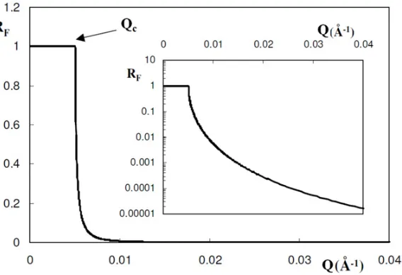
Figure 2. Linear-linear representation and logarithmic-linear representation (inset) of the Fresnel reflectivity as
function of Q for Nbs=2.07 10−6Å−2(interface air/silicon).
where qcand qsare obtained from:
q2
s =4Nbs (22)
qs2 =q2−4Nbp =q2−qc2 (22’)
qcis the critical wavevector that separates total reflection (below qc) from partial reflection where
a part of the beam is refracted beam (above qc). At qc, the wave propagates only at the surface, parallel
to it. The measurement of qcenables the measurement of Nbs(this is another way or writing Eq. (14) in
Sect.2.1).
Please note that, far from the critical angle (qqc), RF ∝(1/q)4. This means that the decay of
the reflectivity is always very fast whatever the layer at the surface (see the representation of Fig.2in linear scale). The NR curves R=f(q) are thus traditionally represented in logarithmic-linear scales or logarithmic-logarithmic scales, as in the inset of Fig.2. Another convenient way of representation is the
Fresnel representation R(q)q4=f(q) for which the q4term compensates the intrinsic q−4decay of the
NR curve to highlight the features coming from the layers at the interface (see the experimental data in the part 4 devoted to the examples). A last possible useful representation is to show R(q)/RF(q)=f(q).
2.4 The case of an homogeneous layer on a substrate
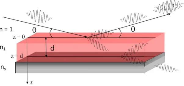
Let us now consider that there is a single homogeneous layer of thickness d at the surface of the perfectly flat substrate whose thickness is considered as infinite of the previous section (Fig.3). The three media are respectively the air (n=1), the layer of refractive index n1 and scattering length density Nb1and
the substrate of index nsand scattering length density Nbs. The air/layer interface is set at z=0 and the
layer/substrate interface is set at z=d.
On such a system a part of the incident wave will be reflected on the first interface at z=0 and a part will be transmitted for q>qc. Also a part of this last transmitted wave will be reflected on the second
Figure 3. Homogenous layer on a substrate.
their phase which is directly linked to their difference of optical path and thus to the thickness of the layer. It therefore appears qualitatively that the reflectivity curve will exhibit interference fringes that enable the measurement of the layer.
After a few calculations the reflectivity writes:
R=
cos(2q1d)
1+ qs q 2
−q1
q
2
−qs q1
2
+1−4qsq +
qs q
2
+q1
q
2
+qs q1
2
cos(2q1d)
1+ qs q 2
−q1
q
2
−qs q1
2
+1+4qsq +
qs q
2
+q1
q
2
+qs q1
2 (23)
It appears on such an equation that the curve of R as function of q will exhibit oscillations whose frequency is given by 2q1d=m×2(m is an integer). This is the Bragg relationship corrected from the critical angle:
2d
sin2
m−sin2c=m (24)
These oscillations are called the Kiessig fringes. Figure4 presents the characteristic NR curve of a system made of a single homogeneous layer on a substrate.
2.5 Roughness and interdiffusion
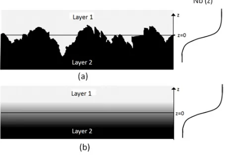
A physical system is described by a profile of scattering length density Nb(z) that is function from the distance to the surface of the substrate. Up to now, we have always considered that the interface between the layer p and the layer p+1 was perfect without any heterogeneity and showed a discontinuity from Nbp to Nbp+1 (step function). In practice, the interfaces are never so abrupt because of two different
physical phenomena: (i) roughness and/or (ii) interdiffusion (see Fig. 5). The roughness accounts from the fact that the passage from one layer to the next is not always at the same distance from the surface z from one area of the surface to another. The interdiffusion accounts from the fact that two materials making two successive layers often mutually diffuse slightly one to each other, which creates a smooth transition.
Figure 4. Reflectivity R calculated for a layer of nickel (Nb=9.4 10−6Å−2) of thickness 500 Å on silicon (Nbs=2.07 10−6Å−2).
Figure 5. (a) Schematic representation of roughness; (b) schematic representation of interdiffusion. The profiles
represented on the right shows the effective Nb(z) profile averaged on the whole surface.
orientations which make some neutrons being reflected out of the specular plane. This does not happen in case of interdiffusion.
Both kinds of interface will be simulated by the same error function:
erf
z−zp/p+1
p/p+1
= √2
(z−zp/p+1)/p/p+1
0
e−t2dt (25)
where p/p+1 is the interface between two successive layers. The curve that shows such an error function has an inflection point in zp/p+1.p/p+1 is the inverse of the tangent’s slope of the curve at zp/p+1. The
thickness of the interface is given by 2p/p+1.
Figure 6. Influence of the roughness on the NR curve calculated on a 500 Å nickel layer deposited on a silicon
substrate. Thick line:s=air=0 Å; thin line:s>0; Dotted line:air>0.
that writes:
DW =exp−4qpqp+12p/p+1
(26) where qpand qp+1are given by equation (ex17).
Another method to take into account roughness is to discretize the density profile in a large number of layers having a low variation of the Nb from one layer to another. However, the calculation time may become very long.
Figure6shows the effect of roughness/interdiffusion on the NR curve calculated in case of the single layer reflectivity of nickel of thickness 500 Å on silicon substrate already presented in Fig.4.
2.6 Data modeling
As mentioned in paragraphs 2.2 to 2.4, it is possible to numerically calculate recursively the reflectivity of a system with n layers if the thickness and the scattering length density of each layer is known, taking into account the roughness at each interface between two adjacent layers by the optical matrix method. The data modeling is then achieved by fitting numerically the calculated NR curve for the studied multilayers system to the experimental curve. The parameters of the fits are the respective thicknesses and scattering length densities of the layers, as well as the roughness of the interfaces. The experimental resolution has also to be taken into account in the simulation (see paragraph 3.2 for calculation). When the scattering length density profile perpendicular to the surface Nb(z) is continuous (as in the case of the adsorption profile of a polymer in solvent at an interface for example), such profile can simply be discretized. As the NR is averaged on the whole surface of the sample, the scattering length density of a layer that contains two types of objects (two polymers in a melt, some molecules dissolved in a solvent, etc.) is the average of the scattering length density of the objects weighted by volume†.
†Example: the case of polymers in a solvent. If the polymer volume fraction ispolyin a given layer, the Nb of the layer is:
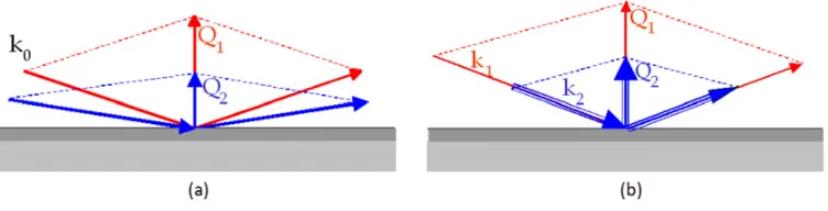
Figure 7. Principle of neutron reflectivity: (a), 2: measurement at variableand fixed; (b) time of flight: measurement at fixedand variable.
There exists however an important problem for the data modeling associated to the fact that the NR curves are cannot be inverted in direct space because only the intensity is measured and not the phase. It is indeed possible to show theoretically that a set of different profiles in direct space give the same NR curve. It is thus important to have a rough idea of the system being studied, as blind treatment can lead to. . . curious results! Besides, owing to the poor fluxes provided by the neutron sources, the error bars are often rather large in an experiment, which makes the distinction between two close profiles sometimes impossible. In order to obtain unambiguous results, several strategies can be implemented. The first one is obviously to make complementary experiments with other techniques that enable to arbitrate between several possible profiles. It is also important to check that the profiles are consistent from a physical point of view, for instance by verifying the volume conservation if one probes the evolution of the profile of a polymer layer as a function of an external stress. Then two strategies specific of NR can be envisaged: (i) When possible, it is possible to use several experimental neutron contrasts for a given physical profile, for instance for measurements in solvent. The obtaining of a unique profile that fits all experiments simultaneously in the different contrasts conditions enables to assess the real profile with confidence (1). This technique is very popular. (ii) Another way of changing the contrast is to place a magnetic layer below the layer to be studied and to perform polarized NR. The advantage here is to get two contrasts conditions on a unique sample but the price to pay is the addition of a layer that make the system more complex (8).
3. Experimental aspects of neutron reflectivity measurements
3.1 Spectrometers
3.1.1 The Different kinds of spectrometers
There exists two ways of measuring the reflectivity of a sample as a function of the scattering vector Q=4sin/(see Fig.7).
The most simple (, 2) is similar to a 2-axis diffractometer and uses a fixed wavelength lying between 1.5 Å and 6 Å. It is suited to continuous neutron sources, id est reactors. The neutron beam, polychromatic at the reactor outlet, is made monochromatic upstream of the sample by a monocrystal, collimated, and sent on the sample in grazing incidence. One measures then the reflected beam, step by step, by rotating the sample of an angleand the detector of 2. The illumination of the sample varies from one angle to another and has to be taken into account in the data reduction. Such a geometry is also used for measurements with X-rays.
NR that it is very often used reactors. As it has a mass, the neutron moves at a finite length, linked to its wavelength via the De Broglie relationν=h/mwhere h is Planck constant and m the neutron mass. For the cold neutrons used in the experiments (with a typical wavelength ranges between 2 and 20 Å), the speed of neutrons lies between a few 100 m/s and a few 1000 m/s. This permits to measure the wavelength of a given neutron within a polychromatic neutron beam by separating the neutrons of different wavelengths of a neutron pulse through their speed, the fastest neutrons moving faster than the slower ones. The pulse, which is spontaneously created on a spallation source, is created by a chopper on a reactor source. The neutrons beam is sent in grazing incidence on the sample and the chopper defines origin of times t0=0 (the “starting line”). On measures then the timet taken by the neutron
to reach the detector located at the distance L from the chopper to determine the wavelength (via= h/mL*t)‡. The rotation of the chopper is chosen so that the slowest neutrons of a pulse arrive sooner on the detector than the fastest neutrons of the next pulse. Measuring the coefficient of reflection is simple: The white incident polychromatic beam has to be first measured without reflection prior to the measure to determine its energy dispersion. The intensity measured for the reflected beam has then to be divided by this incident white beam for every value of.
The time-of-flight method is extremely convenient for some geometries of measurement, in particular those at the air/liquid, because it does not force to rotate the sample (and to make it flow. . . ) or to use a deviating mirror. Moreover, all the points of reflectivity curve are measured in the same time, which removes any incertitude on the possible aging of the sample during measurement, a feature that often occurs in soft matter. Reciprocally, this method allows kinetics measurements that have become very popular these last years with the development of high-fluxes spectrometers such as Figaro at ILL that enable to measure a given NR spectrum in a few minutes.
In an NR experiment, the incident angle on the surface to study is always very weak, ranging typically from 0.5 to 5◦. Given the typical wavelengths of the incident neutrons (∼3 Å–25 Å), the range of scattering vectors lies between 0.003 Å−1and 0.3 Å−1. The typical thicknesses that can be measured
in standard conditions vary then from around 10 Å to 2000 Å.
3.1.2 An example of Time-of-Flight Spectrometer: EROS at LLB
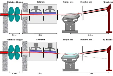
A full description of this horizontal spectrometer can be found in reference (9). It is shown on Fig.8. Briefly, the neutrons produced by the Orphée reactor (CEA Saclay) are thermalized by a liquid hydrogen cold source (T=20K). A bended neutron guide conveys them up to the spectrometer located at around 30m from the source. A “white” beam containing a broad spectra of wavelengths is then available at the chopper position (in practice from 3 to 25 Å). The chopper with a raw/constant resolution is made of two-rotating wheels covered by gadolinium, a neutron absorber, pierced by two large slits. The distance and phase between the two wheels enable to change the/from 1% to 13% depending on the resolution request. The beam passes then through a collimator under vacuum that is 1.8 m. The aperture of the horizontal entrance and exit slits may be varied from 0.2 mm up to several cm (in standard conditions, on uses apertures lying from 1 mm to 3 mm). Two neutron supermirrors can be inserted within the collimator to deviate the beam for air/liquid measurements. The beam is then reflected by the sample tilted of an angleand measured by a3He single detector.
The maximal angle that can be reached is 5◦, which enables to cover a scattering vector range from 0.003 à 0.3 Å−1(measurements below 0.3◦are practically almost impossible because the reflected
beam has to be separated from the incident non-deviated beam). A measurement at one angle allows
Figure 8. Scheme of the EROS reflectometer, from reference (9). Top: Geometry of measurement for air/solid measurements; Bottom: Geometry of measurement for air/liquid measurements.
to cover around one decade in q. If this is sometimes sufficient for the desired measurement, most of times 2 or 3 different angles are used to cover a broad q-range. The actual minimal reflectivity in air/solid geometry that can be obtained is a few 10−7. For measurements involving liquids, this
limit is superior to 10−6 because of incoherent scattering (see Ref. (9) for more details). The vertical
position has to be adjusted as a function of the chosen angle. If h0 are hD are the respective
position of the direct beam and of the detector at the distance L from the chopper, the angle of a measurementis given by: tan 2= hD−h0
DS_Dwhere DS_Dis the distance from the sample to the detector
(Fig.8).
The principle of alignment is simple. The angle of work has to be chosen first such as part of the neutron beam is in total reflection (if the neutron contrast conditions enable it) thanks to the formula (14). The height position is then fixed. The sample has than to be placed within the beam and rotated with the goniometer up to recording the maximum of neutrons on the detector. This is exactly similar to what you were doing when you were a child when you rotated your watch to reflect the light (the neutrons) in the eye of someone (the detector). . . For air/liquids measurements, the angle of work is fixed by the deviating supermirrors within the collimator (see Fig.8b).
The typical duration of the acquisition time depends on the minimal reflectivity that is requested. If it is of the order of 10−5, 30 min to 1h are necessary to obtain a correct statistics but this time has to be
extended up to∼4 hours to reach a few 10−6. These typical measurement times are given for sample of around 10 cm2. Such large surfaces can be indeed be used because the collimations used are large (see below).
Figure 9. Divergence of incident beam when the effect of the earth gravity on the neutrons path is neglected.
3.1.3 Angular resolution
Owing to the collimation, the incident beam on the sample has a divergence that induced an enlargement of the beam and that has to be taken into account in the calculation, the expressions presented in the precedent part for the reflectivity being calculated for incident beam without divergence. This is achieved by the convolution of the calculated function by an apparatus function f(,0) centered
in 0. This function can be either a triangle function or a square function.
R/(q)=
R
qsin0 sin
f(0−,)d (27)
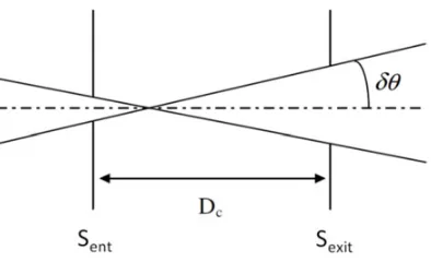
The divergence of the incident beamand the angular resolution/are set by the apertures of the entrance and exit slits of the collimator and by the collimator length Dc. If the earth gravity is neglected,
the trajectory of the beam is supposed straight and the divergence by: tan = (Sent+Sexit)/2Dc.
The calculation of the resolution for an angle of 1◦, for slits Sent= 2 mm and Sexit 1 mm and for
Dc=1800 mm give :=0.047◦and/=4.7% (characteristic values used on EROS).
3.2 Samples and possible geometries of measurements
3.2.1 The different geometries of measurements
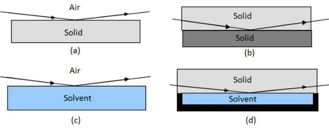
Figure10shows the four types of interfaces that is it possible to study: air/solid, solid/solid, air/liquid solid/liquid and the associated geometries. For the solid/liquid geometry, the beam must necessarily cross the solid and not the liquid (considered here as either water or an organic solvent). It is indeed impossible for a neutron beam to cross several centimeters of liquid. Indeed, for some reasons that will be not detailed here but that are described in the introduction course of this volume, a neutron can be scattered by some atoms with a constant probability over 4independently from the positions of these atoms (incoherent scattering). The incoherent scattering cross-section is very high for hydrogen1H and
some elements of the periodic table (vanadium. . . ), rather important for2H deuterium, and null or very
weak for most elements of the periodic table. The incoherent scattering of a liquid is thus very important, which in turn decreases the transmission of the beam. For example, the transmission by a neutron beam at=6 Å is only 0.5 through 1 mm of H2O and 0.8 through 2 mm of D2O.
3.2.2 Samples
Figure 10. The four possible kinds of measurements in Neutron Reflectivity: (a) air/solid interface; (b) solid/solid
interface; (c) air/liquid interface; (d) solid/liquid interface.
that it is similar to an increase of the divergenceof the beam. This divergence could be taken into account by an increase of the effectivewithin the resolution function during the data modeling. Solid samples must be rigid enough not to deform mechanically under internal stresses. One must also ensures that samples do not contain atoms that strongly absorb neutrons (Li, B, Gd. . . ) or have an important incoherent scattering cross-section (V...) to avoid the decrease of flux in general and the radiological activation of samples in case of absorption. This is especially important for the solid incoming media that has to be crossed in solid/liquid or solid/solid geometries. The absorption and incoherent scattering cross-sections can be found in neutron periodic tables (6).
The raw measured reflectivity is proportional to the surface of the sample illuminated by neutrons prior to the data reduction where it is normalized to unity for total reflection. If possible, the surface of the sample has to be maximized in order to get a good signal-to-noise ratio with reasonable acquisition times. Ideally, the best is to have an overall surface of sample that is higher than the area illuminated by neutrons during experiment (some cm2 depending on the collimation and samples). The surfaces
can be decreased at cost of increasing counting rate but is must avoided to decrease down to 1 cm2
(actually the lowest surface ever probed on EROS were∼0.15 cm2 but the minimal reflectivity was 10−3 (10). It is not possible to go down to such small surface for measurements at air/liquid interface (see below).
Silicon wafers or quartz crystals are very commonly used as model substrates for solid. They must be thick enough not to deform mechanically (a minimum of 1 mm is required for silicon wafers)). The silicon wafers are especially suited to design model substrates for NR and are used in∼90% of experiments on solid substrates for non-magnetic systems, both at air/solid interface and solid liquid interface because they have several properties that make them unique for NR: (i) they are nearly transparent to neutron because their incoherent scattering cross-section is null and their absorption cross-section is very weak (7 cm of silicon are required to attenuate a neutron beam at =6 Å by a factor 2!); (ii) their lack of incoherent scattering do not any additional background scattering; (iii) they have an excellent mosaicity with an rms roughness of a few Å; (iv) their chemical surface (Si-OH groups) lends itself to many chemical modifications which are easy to achieve at laboratory without any specific material in order to design hydrophilic surfaces, hydrophobic surfaces, charged surfaces, functionally-terminated surfaces. . . ; (v) last but not least, they are rather cheap and easy to purchase at silicon manufacturers owing to their importance in electronic industry.
perturb the measurement because they have an impact on the NR curve only for very small reflectivities that cannot be reached with neutrons.
3.2.3 Samples environments
Thanks to the poor absorption of neutrons by matter and in particular by some metallic elements, it is easy to design various samples environments for in situ experiments: liquids cells, cells with solvent circulation baths, Langmuir trough, ovens, cryomagnets, pressure cells, temperature controllers, etc.
It is advised to contact people from facilities prior to experiments to check that the equipment can be used with the kind of sample to study. It is also of course possible to design its on sample environment for specific experiments.
3.3 Access to the spectrometers
As NR is a growing expanding technique, there are reflectometers in all of the large neutron facilities. A recent special issue on neutron instrumentation has focused on the reflectometers recently released or upgraded and new techniques of instrumentations in NR (11). In France, there exist two neutron facilities, the Institut Laue Langevin (ILL) in Grenoble which is an European source run jointly By France, Germany and United Kingdom (12) and the Laboratoire Léon Brillouin (LLB), the French national source which is located in Saclay 30 km from Paris (13). There are actually 3 reflectometers at ILL (FIGARO dedicated to soft matter and biophysics, D17 for multipurpose measurements and SUPERADAM for magnetic studies) and 2 at LLB (EROS, an horizontal versatile multipurpose instrument that will be soon be upgraded in HERMES, and PRISM for magnetic studies).
All of these spectrometers are available free of charge by the whole scientific community. The beamtime is allocated by a committee of experts on the basis of proposals experiments. The proposals can generally submitted twice a year (the deadlines depend from one facility to another). Information on formalities claims experience can be found on the websites of the facilities. All results obtained with allocated beamtime must be published without restriction.
It is also possible to perform experiments whose results will remain confidential, for industrial applications for example. The beamtime is no longer free and the contract allowing access to the beam must be negotiated directly with the facilities.
Finally, although neutron scattering is poorly taught at university, there exist some neutron schools open to pHD students, post-doc fellows and academic researchers with practicals on the spectrometers that enable to get familiar with NR. In France, there are two recognized recurrent formations: Hercules which combines X-rays and neutrons in association with several facilities (in English) (14) and les FANs
du LLB specifically on neutrons at LLB (in French) (13).
4. Examples of neutron reflectivity related to materials for energy
4.1 Asphaltene adsorption mechanism under shear flow probed by in situ neutron reflectivity measurements
The results presented here all come from the reference (15). This work was a collaboration between
IPFEN, the French institute for research on oil, and LLB.
(16) formed by an aromatic dense core and a highly aliphatic shell (17) that is described in the SANS
course of this volume). Due to their surfactant properties, these clusters are able to adsorb solid-liquid
interfaces (18), which may have important effects such as wettability alteration in petroleum reservoirs. During oil production, the pressure decrease near the wellbore can also induce the flocculation of the asphaltene fractions resulting in reduction of the porous volume by pore blockage and/or multilayer formation. NR was then used to get a description at of these adsorption and deposition mechanisms at the nanometer scale.
In steady state, it was shown that the adsorbed asphaltene layer is a solvated monolayer with a thickness of the order of the size of the nanoaggregate in bulk in good solvent, both for hydrophilic and hydrophobic solid surfaces (19). When a bad solvent is progressively added, the asphaltene adsorbed layer keeps its monolayer structure as long as the bulk flocculation threshold is not reached. Above the threshold, the size of the asphaltene adsorbed layer growths and forms a multi-layer structure with time. This first study however did not mimic properly the real situation in porous media or pipes because crude oils undergo a strong laminar shear flow during their transport. In order to go further on the description of such real situation, the kinetic evolution of the structure of the adsorbed layer of asphaltene in bad solvent at a hydrophilic solid/liquid interface in presence of a shear flow controlled by a cone/plate rheometer was probed, as described in the following.
4.1.1 Material and methods
The asphaltenes clusters (Mw of 200000 g/mol and Rg of 84 Å) were initially dissolved in a good
solvent, xylene, after their extraction from crude oils. Deuterated xylene (5.91 10−6Å−2) was used
to obtain a good contrast with respect to the silicon substrate (2.07 10−6Å−2) and to asphaltenes (1.40 10−6Å−2) , as well as to lower incoherent scattering from solvent. The addition of bad solvent was done by adding deuterated dodecane (6.71 10−6Å−2) in the solution to reach a 34%/66% xylene/dodecane ratio, below the threshold ratio required for bulk flocculation (19). An hydrophilic wafer was used as substrate.
Figure11a shows a schematic view of the experiment assembly. A controlled stress rheometer with a cone/plate geometry was placed on the EROS spectrometer just after the collimator, with its plateau at a fixed angle to the incident neutron beam (Fig. 11b). The measurements were performed at the silicon/mixture of xylene and dodecane interface in a sealed cell especially designed to be mounted on rheometer, whose inner diameter was slightly higher than the one of the plate of the rheometer in order to ensure a homogeneous shear within the cell. The neutron beam was entering through the silicon. It was possible to measure shear rates ˙=0/up to 2600 s−1. The reflectivity curves were recorded by
slices of 30 minutes, a time sufficient for an acquisition with a good statistics.
4.1.2 Results and discussion
Two different shear rates ˙(1200 s−1and 2600 s−1) were probed, as well as the references measurements
in good solvent and after addition of bad solvent without shearing. Figure12presents the whole kinetic evolution of the SNR curve obtained at 1200 s−1. An interest reader can find all other experimental
results in (15). Data are presented in the log(RQ4)= f(Q) Fresnel representation to highlight the
evolution of the structure of the asphaltenes layer at the interface. Even after 30 minutes of elapsed time, the thickness of such layer is around∼200 Å, already much larger than the monolayer evidenced in good solvent (∼87 Å, in accordance with the bulk Rg (15)), due to the subsequent adsorption of
Figure 11. (a) Principle of the experiment. The silicon wafer is represented in gray, the cone of the rheometer in
light blue, the deuterated solvent in orange and the asphaltene nanoaggregates in black. (b) Experimental set-up. The neutron beam, schematized in red, outcoming from the exit slit of the collimator, crosses the cell where it is reflected and finally enters a black arm made of B4C used to reduce background placed in the front of the detector (not visible in the picture). Inset: picture of the cell specifically designed for the experiment (top view). Taken from reference (15).
It was chosen to model the adsorbed layer as a multilayer, an approach that enables a confident determination of the overall volume fraction at the surface and its decay down to overall thickness of the layer. The SLD profiles corresponding to the modeled SNR curves are presented in Fig.12b and are converted into asphaltenes volume fraction profiles (Fig.12c). The layer is poorly solvated at the vicinity of the surface sinceasphaltenereached∼85%.asphaltene decays then down to∼40–45% at the
top of the layer. The volume fraction profile has almost the same shape as time passes, showing that the inner structure of the asphaltene adsorbed layer remained unchanged.
Finally the surface excess were obtained from the integral of the profiles that enable to extract the excess mass (in mg/m2). They are shown in Fig. 13 as function of time for all the different experiments where they are compared with complementary experiments performed by Quartz Crystal Microbalance (only the raw data, id est the shift of frequency of the microbalance f are presented).
It shows a clear-cut linear behavior with time: the increase of amount of asphaltenes deposited is much higher at 0 s−1than at 1200 s−1, the adsorption is therefore shear-limited. The surface excess
increases initially almost linearly with time for a given shear rate. It slows down at longer time probably due to the competition between the adsorption at the interface induced by bulk flocculation and the desorption due to the applied shear rate. The adsorption is strongly limited at 2600 s−1since the surface
excess is around twice lower at 2600 s−1than 1200 s−1at long times.
4.2 Phase separation-driven stratification in conventional and inverted P3HT:PCBM organic solar cells
The results presented here all come from the reference (20) and were performed by a team specialized on polymers for electronics at LCPO laboratory (Bordeaux, France).
Figure 12. Kinetic evolution of the SNR experimental curves at 1200 s−1, and the corresponding fits. For clarity, all curves were shifted in intensity, except for t=30 min. (b) SDL profiles corresponding to the fits of Fig. 12a. (c)asphatene=f(z) profiles corresponding to the fits of Fig.3(b). Taken from reference (15).
Figure 13. Comparison of the kinetic evolution of the surface excess of asphaltenes with or without appliance of
shear derived from neutrons with raw QCM data. Taken from reference (15).
Figure 14. The reflectivity curves collected for the as cast and annealed P3HT:PCBM blends spun on:
(a) PEDOT:PSS and (b) TiOx layers, to mimic the films incorporated in conventional and inverted solar cells respectively.The curves that correspond to the unannealed films were shifted vertically for clarity. Taken from reference (20).
charge transport to the electrodes should be promoted through a co-continuous network that provides pathways to the corresponding electrodes. While much work is directed towards tuning the in-plane active layer morphology, it is of great importance to determine if there are concentration gradients and heterogeneities perpendicular to the film plane. Indeed, in a photovoltaic cell the photo-generated charges should travel perpendicular to the plane of the film to reach the electrodes. Thus, if concentration heterogeneities exist next to the electrodes, charge harvesting may be either inhibited or facilitated. The aim of the study was then to determine by neutron reflectivity the concentration-depth profiles of blend films of the electron- donor poly(3-hexylthiophene) (P3HT) and the electron-acceptor phenyl-C61-butyric acid methyl ester (PCBM,), which is the most well-studied system for organic photovoltaic applications. The P3HT:PCBM active blends were respectively spun cast on the top of two different kinds of layers: (i) a film made of one part poly(3,4-ethylenedioxythiophene) to six parts poly(styrene-4-sulfonate) (PEDOT:PSS) that is a common hole transport layer for conventional solar cells and (ii) titanium oxide (TiOx), which is widely used as an electron transport layer, suitable for inverted solar cells. The two layers were themselves deposited on silicon wafers.
Neutrons are a unique tool for studying the P3HT:PCBM blends due to the significant contrast between the two materials; P3HT has an SLD of 0.67 10−6Å−2 while PCBM has an SLD of 4.34 10−6Å−2. These SLD are also different from the ones of PEDOT:PSS (0.67 10−6Å−2) and TiOx (1 10−6Å−2). Figure14shows the results obtained in Fresnel representation for both geometries, either
for as-cast and annealed films (165◦C for 20 min). All curves show large oscillations arising from the different layers at the surface. For both systems, the fringes are much more marked for the annealed films, pointing out that is less interdiffusion within the films. Figure 15a and Fig. 15b shows the scattering length profiles corresponding from the fits of the NR curve. Finally, the PCBM volume fraction distribution within the annealed P3HT:PCBM blends was specifically extracted from these SLD profiles, as shown in Fig.15c.
Figure 15. The neutron scattering length density profiles derived by fitting the reflectivity curves of the as cast and
annealed P3HT:PCBM blends spun on: (a) PEDOT:PSS and (b) TiOx layers. The transport/active layer interface is set to z= 0. (c) The PCBM volume fraction distribution within the annealed P3HT:PCBM blends cast on PEDOT:PSS and TiOx transport layers. Taken from reference (20).
The authors thank the organizers of the “Neutrons and Materials for Energy” school Monica Ceretti, Marie-Hélène Mathon, Clemens Ritter and Werner Paulus for their kind invitation to participate to this special issue.
References
[1] J. Penfold, R. K. Thomas, The application of the specular reflection of neutrons to the study of surfaces and interfaces, J. Phys.: Condens. Matter. 1990, Vol. 2, 1369–1412.
[2] T.P. Russell, X-ray and neutron reflectivity for the investigation of polymers. Materials Science
Reports, 1990, Vol. 5(4), 171–271.
[3] N. Torikai, N. L. Yamada, A. Noro, M. Harada, D. Kawaguchi, A. Takano, Y. Matsushita, Neutron Reflectometry on Interfacial Structures of the Thin Films of Polymer and Lipid. Polymer Journal, 2007, Vol. 39, 1238–1246.
[4] Wacklin, H.P. Neutron reflection from supported lipid membranes. Curr. Opinion in Coll. Inter. Sci. 2010, Vol. 15(6), 445–454.
[5] C. Fermon, F. Ott, A. Menelle. Neutron reflectivity. J. Daillant and A. Gibaud (eds) X-Ray and
Neutron Reflectivity: Principles and Applications, Springer Lecture Notes in Physics, Berlin,
1999, 163.
[6] Sears, V.F. Neutron scattering lengths and cross sections. Neutron New,. 1992, Vol. 3, 26–37.
[7] http://www.neutron.anl.gov/reference.html.
[9] F. Cousin, F. Ott, F. Gibert, A. Menelle. EROS II: A boosted Time-of-Flight Reflectometer for Multi-purposes Applications at the Laboratoire Léon Brillouin. Eur. Phys. Jour. Plus, 2011,
Vol. 126, 109.
[10] F. Lechenault, C.L. Rountree, F. Cousin, J.-P. Bouchaud, L. Ponson, E. Bouchaud. Evidence of deep water penetration in silica during stress corrosion fracture. Phys. Rev. Lett., 2011, Vol. 106, 165504.
[11] A. Menelle, G. Fragneto. Progress in neutron reflectometry instrumentation,. Eur. Phys. Jour.
Plus, 2011, Vol. 126, 106.
[12] http://www.ill.eu/. [13] http://www-llb.cea.fr/. [14] http://hercules-school.eu/.
[15] Y. Corvis, L. Barré, J. Jestin, J. Gummel, F. Cousin. Asphaltene adsorption mechanisms under shear flow probed by in-situ neutron reflectivity measurements. Eur. Phys. Jour. Special Topics, 2012, Vol. 213, 295–302.
[16] L. Barré, S. Simon, T. Palermo. Solution properties of asphaltenes. Langmuir, 2008, Vol. 24, 3709. [17] J. Eyssautier, P. Levitz, D. Espinat, J. Jestin, J.Gummel, I. Grillo, L. Barré. Insight into asphaltene nanoaggregate structure inferred by small angle neutron and X-ray scattering. J. Phys. Chem. B, 2011, Vol. 115, 6827.
[18] S. Acevedo, M.A. Ranaudo, C. Garcia, J. Castillo, A. Fernandez, M. Caetano, S. Goncalvez. Importance of asphaltene aggregation in solution in determining the adsorption of this sample on mineral surfaces. Colloids Surf. A, 2000, Vol. 166, 145.
[19] N. Jouault, Y. Corvis, F. Cousin, J. Jestin, L. Barré. Asphaltene adsorption mechanisms at the local scale probed by neutron reflectivity: transition from mono to multilayer growth above flocculation threshold. Langmuir, 2009, Vol. 25(7), 3991–3998.