Software Fault Prediction Model for Embedded
Systems: A Novel finding
Pradeep Singh1, Shrish Verma2 1,2
National Institute of Technology, Raipur, India
Abstract— Software testing plays a vital role in software development especially when the software developed is mission, safety and business critical applications. Software testing is the most time consuming and costly phase. Prediction of a modules info fault-prone and non fault prone prior to testing is one of the cost effective technique. Predicting a safe module as faulty increases the cost of projects by more cautious and better-test resources allocation for those modules, whereas prediction of faulty code as fault free code end up in under-preparation and may leave modules untested this may cause accidental failure and lead towards massive loss . In this research, we present a novel fault prediction technique that reduces the probability of false alarm (pf) and increases the precision for detection of faulty modules. The general expectation from a predictor is to get very high probability of false alarm (pf) to get more reliable and quality software product. We have taken embedded systems software for this study and the goal is to predict as many faulty modules as possible. In this paper we apply a supervised discretization for pre-processing and clustering based classification for prediction of a modules info prone (fp) and non fault-prone (nfp) modules. To evaluate this approach we perform an extensive comparative experimental study for the effectiveness of our method with benchmark results for the same embedded software’s. Our fault prediction model produces better results than the standard and benchmark approaches for software fault prediction.
Results from our proposed model significantly decreases probability of false alarm (pf) down to 9% while increasing precision and balance rates at 68% and 79% respectively.
Keywords Software fault prediction, supervised discretization, and software metric.
I. INTRODUCTION
The demand of highly reliable and secure system is increasing day by day. To fulfill these demands by the ever-increasing power of computing devices, systems are growing complex. Due to the complexity of these systems, effort and cost incur in development is increasing. Software complexity is the main source of failure and potential hazards. High quality software within allocate budget requires a careful planning and cost effective use of testing resources. Mission critical or safety and business critical system needs more reliability and therefore requires more testing time and resources.
Testing phase is the most expensive, time and resource consuming phase of the software development lifecycle requires approximately 50% of the whole project schedule [1, 2]. So an effective and intelligent test strategy can minimize the time of testing by using resources efficiently. Various methods for minimization of testing effort, inspections [3], manual software reviews or automated
models [4], [5] are proposed. A panel at IEEE Metrics 2002 [6] concluded that manual software reviews can find approximately 60% of faults. Automated models proposed for fault prediction are useful tools for software organizations and significantly better in terms of fault detection performance, compared to other verification , validation and testing activities [5][17][18]. These automated models uses static code attributes such as Lines of Code (LOC) and the McCabe/Halstead complexity and other software attributes that can be easily extracted from source code repositories even for large systems.
Software fault prediction uses various method-level static code software metrics such as Halstead , Mc- Cabe metrics etc. to categorize modules and predicting them either fault-prone(fp) or non-fault prone( nfp) modules by using classification model derived from the data of projects. In software fault prediction problems, we have X = {x1, x2, …
xn}where x represents software module that is characterized
by software metrics and Y = {fp,nfp} ,where an unknown system S predictive model transforms from instances X to predicted classes Y; Y = S(X). Prediction models based on software metrics, can estimate number of faults in software modules as well as which module is faulty. So the predictive models are easy to use and faster to run for highlighting fault-prone modules compared to inspections [4],[5],[7].Fault predictors models are useful tools for software organizations to manage their testing resources effectively through focusing on fault-prone software modules to mprove software quality. Many researchers have already worked for fault prediction model and various software metrics and techniques like linear regression, decision trees, neural networks and Naive Bayes classification have been analyzed [5][8][9].
ANN, Voting Feature Intervals (VFI) ,Naïve Bayes and other ensemble( Ens2) which uses Naive Bayes and VFI algorithm .
In the following section, models used for defect prediction are explained. After describing the experimental design, results, and conclusions will be given.
II. RELATED WORK
Researchers have used various methods such as statistical analysis, regression, Genetic Programming [11], Decision Trees [12], Neural Networks [13], Naïve Bayes [5], Case-based Reasoning [14], Fuzzy Logic [15] and Logistic Regression [16] for software fault prediction.
Elish et al. [17] investigated the performance of Support Vector Machines (SVMs) and found SVM better than, or at least is competitive against the other statistical and machine learning models in the context of four NASA datasets. They compared the performance of SVMs with the performance of Logistic Regression, Multi-layer Perceptrons, Bayesian Belief Network, Naive Bayes, Random Forests, and Decision Trees. They used correlation based feature selection technique (CFS) to down select the best predictors out of the numbers of independent variables in the datasets. Catal et al. [18] investigated effects of dataset size, metrics set, and feature selection techniques and found Random Forests provides the best prediction performance for large datasets and Naive Bayes is the best prediction algorithm for small projects. Tomaszewski [19] have conducted Statistical models vs. expert estimation for fault prediction and found statistical techniques performed superior to locate software fault than an expert estimations approach stating that” When it comes to comparing both methods we found that statistical models outperformed expert estimations”.
Gondra’s [20] experimental results showed that Support Vector Machines provided higher performance than the Artificial Neural Networks for software fault prediction. Quah [21] used a neural network model with genetic training strategy to predict the number of faults, the number of code changes required to correct a fault, the amount of time needed to make the changes and he proposed new sets of metrics for the presentation logic tier and data access tier. Turhan et al. [22] analyzed the effects of preprocessing of software defect data from NASA with PCA ,subset selection and weighted Naive Bayes and concluded that either pre-processing software defect data with PCA or using weighted Naive Bayes should be preferred rather than subset selection for Naïve Bayes models.Menzies et al. [5] reported that Naive Bayes with logNums filter achieves the best performance in terms of the probability of detection (pd-71%)and the probability of false alarm (pf-25%) values which is are much larger than their prior results of mean (pd, pf)=(36%, 17%). They also stated that there is no need to find the best software metrics group for software fault prediction because the performance variation of models with different metrics group is not significant and the choice of learning method is more important. Almost all the software fault prediction studies use metrics and fault data of previous software release to build fault prediction models, which are called ‘‘supervised learning” approaches in
machine learning community. There have been discussions on finding the best classifier for fault predictors. Lessmann et al. [35] argued that their 15 best performing classifiers were statistically indistinguishable from each other in terms of the area under the receiver operating characteristic (ROC) curve. The authors did not use any filtering or transformation techniques. Instead, they used the algorithms on the original data to measure their effectiveness on detecting defect-prone modules. Ayse et al [23] used multiple predictors (classifiers) to produced better results for locating defects they used an ensemble of classifiers to predict defects in embedded software and achieved probability of detection (pd-76%) and the probability of false alarm (pf-22%) for ensemble (Ens1) which combines ANN, Voting Feature Intervals(VFI) and NB and probability of detection (pd-69%) and the probability of false alarm (pf-17%) by ensemble (Ens2) which uses only Voting Feature Intervals(VFI) and NB.
We used embedded data from promise repository [25] which is an open source repository for fault data. Therefore; all projects used in this study are available online. So, this work can easily be repeated, improved or refuted by other researchers [24][22] .We present a defect prediction model based on cluster based classification for embedded and mission critical software results reveal probability of detection (pd-76%) and the probability of false alarm (pf-9%) which is statistically significant by the earlier models.
III.EXPERIMENTAL DESIGN
From an industrial perspective, software managers aim to decrease their testing efforts while decreasing fault rates, thereby producing high quality real time systems. We observed that cluster based classifiers would detect 76% of the faulty modules with precision of 68%. Also the cluster based classification decreases the false alarms rates. In commercial applications, companies need to employ cost effective oracles, since an increase in false alarms would waste inspection costs by guiding testers through actually safe modules. Therefore, in this paper, our objective is “building a learning-based fault predictor for embedded systems that would decrease false alarms while producing high detection rates’’.
We used a cluster-based classification framework in which fault-prone and not fault-prone modules are grouped into clusters. In our experiment we use supervised discretization as preprocessing technique. We first discretized the data using entropy based supervised discretization to divide the continuous attributes into the range intervals. It makes learning more accurate and faster. After supervised discretization we have applied clustering technique on processed data to build and effective fault prediction model. We evaluated this model on embedded software and then compared this method with a recent study which is based on ensemble classification for the same embedded softwares [23].
As indicated by Shull et al. [43], replications help the software engineering researchers to address internal and external validity problems. These types of studies also lead the research community to build a solid knowledge about the influence of conditions on the experimental results and observations. In this study, we observed a recent study on defect predictors for embedded system by Ayse et al [23] and we have reproduced better results via new techniques in order to find the better approaches for fault prediction .
Lessman et al. [35] reported that data preprocessing or engineering activities such as the removal of noninformative features or the discretization of continuous attributes may improve the performance of some classifiers [35]. For example, Menzies et al. report that their Naive Bayes classifier benefits from feature selection and a log-filter preprocessor [5].
Discretisation is the transformation of a continuous variable into a discrete space, grouping together multiple values of a continuous attribute, and partitioning the continuous domain into a finite numbers of non-overlapping intervals. The task of discretizing an input attribute for classification problems is usually divided into supervised discretisation, when knowledge interdependency between the class level and attribute values is used for the discretization process and unsupervised discretization, when the class values of the instances are unknown or not used. The methods for unsupervised discretization are equal-width and equal-frequency binning. The equal width divides the range of values of a numerical attribute into a pre-determined number of equal intervals. The equal frequency divides the range of values into a pre-determined number of intervals that contain equal number of instances.
Supervised algorithms are maximum entropy [37], Patterson and Niblett [39], statistics- based algorithms like ChiMerge [40] and Chi2 [41].
Fayyad & Irani developed a concept of entropy based partitioning in [36]. We have used entropy based [46][36] discretization before classification.
Fayyad & Irani's approach was developed in the context of decision tree learning that tries to identify a small number of intervals, each dominated by a single class. They first suggested binary discretization, which discretizes values of continuous attribute into two intervals. The training instances are first sorted in an increasing order, and the midpoint between each successive pair of attribute values is evaluated as a potential cut point. The algorithm selects the best cut point from the range of values by evaluating every cut point candidate. For each evaluation of a candidate, the data is discretized into two intervals and the entropy of the resulting discretization is computed. In a given a set of instances S ,a feature A, and a partition boundary T, the class information entropy of the partition induced by T, denoted E(A,T;S)is given by
E(A,T;S)= S1/S Ent(S1 )+S2/S Ent(S2 )
For a given feature A, the boundary Tmin which minimizes the entropy function over all possible partition boundaries is selected as a binary discretization boundary. This method can be applied recursively to both of the partitions induces by Tmin until some stopping condition is achieved. Fyyad and Irani make use of minimal descriptive length Principle to determine stopping criteria for their recursive discretisation process. Recursive partitioning within a set of value S stops if
Gain(A,T;S)<(log2 (N-1))/N+(∆(A,T;S))/N
Where N is the number of instance in the set,S, Gain(A,T;S)=Ent(S)-E(A,T;S),
∆(A,T;S)=log2(3k-2)-[k.Ent(S)-k1.Ent(S1 )-k2.Ent(S2 )],
and ki is the number of class labels represented in the set S.
Since the partitions along each branch of the recursive discretisation are evaluated independently using this criteria, some areas in the continuous space will be partitioned very finely whereas other which has relatively low entropy will be partitioned coarsely.
building .Finally after building clusters mapping is done on the basis of lowest error. A particular class label can be associated with at most one cluster. To overcome the sampling bias we have used M*N-way cross validation where both M and N are selected as 10 [44]. We create 10 stratified bins: 9 of these 10 bins are used as training sets and the last one is used as the test set. We randomize the dataset M = 10 times and create N = 10 sets in each iteration. We apply clustering based classification algorithm on the preprocessed embedded fault dataset. Finally we have compared our result with the Ens1 and Ens2 used by [23] for fault prediction of embedded systems. The pseudo code of the model is shown below in Fig. 1.
Procedure Evaluation data Learning (data, scheme)
Input: data - the data on which the learner is built, AR3, AR4, AR5]
Learners- The learning scheme. [Cluster_based_classification ]
Output Result [D_pd, D_pf, D_prec,D_bal] = D_predictor on TEST pd,pf, precision and balance over M*N way cross validation.
Preprocessing = {supervised discretisation} M=10;N=10;
FOR each data
D_Data = apply supervised discretisation //discretization of data
// construct predictor from D_Data For 1=1 to M
T=Generate N parts of each D_Data For J =1 to N do
Test=T[j] Train=T- T[j]
Model=Apply learning scheme on Train D_Prediction =Apply Model to test End for
End for
//Evaluate predictors on the test data
[D_pd ,D_pf, D_prec, ,D_balance ] = D_ predictor on TEST
End for
Figure 1: Algorithm for Software fault prediction
IV.DATASOURCE
We use data which is publicly available in the Promise Data Repository [25]. The three embedded projects AR3, AR4, AR5 are from Turkish white good manufacturer Software Company. Each data set is encompassed of several software modules, together with their static code attributes and associated corresponding number of faults. After metric and bug data extraction from software repositories , modules that contain one or more bugs were marked as fault prone (fp), and where no bug were reported those modules were treated as non fault prone (nfp). The fault data sets which are taken from promise repository includes LOC counts, several Halstead attributes, McCabe complexity measures as well as various other static code attributes. Individual software metric feature per data set,
together with percentage faulty modules and some general descriptions are given in Table 1.
TABLE 1:DATA SET USED IN THE STUDY
Source No of Module
Features LOC % Faulty
Language
AR3 63 29 5624 12.7 C
AR4 107 29 9196 18 C
AR5 36 29 2732 20 C
A. Performance Measures
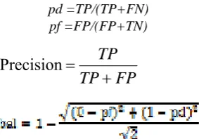
The accuracy and performance of prediction models for two-class problem, defective or not defective is typically evaluated using a confusion matrix. A confusion matrix contains information about actual and predicted classifications done by a classification system. In this study, we used the commonly used prediction performance measures: probability of detection (pd), probability of false alarm (pf), precision (prec), balance (bal) to evaluate and compare prediction models quantitatively. These measures are derived from the confusion matrix.
A confusion matrix
Actual Faulty Module Not Faulty Module
Predicted
Faulty Module TP(True
positive)
FP (False positive) Not Faulty
Module
FN (False
negative)
TN (True Negative)
False alarms, pf, should be 0, meaning that the predictor should never label a fault-free module as faulty. In general, an increase in pd would also increase pf rates since the model triggers more often to achieve the ideal case [5]. To see how close our estimates are to the ideal case, we use a balance metric, which is the Euclidean distance between the ideal point and where we are on the ROC curve in reality. Precision is also known as correctness. It is defined as the ratio of the number of modules correctly predicted as defective to the total number of modules predicted as defective.
pd =TP/(TP+FN) pf =FP/(FP+TN)
The higher the precision, the less effort wasted in testing and inspection. It has a strong relation with pd and pf, such that when pd is fixed for a dataset, pf rate is controlled by precision and the class distribution of the data [5]
FP
TP
TP
V. RESULTS
A novel approach Cluster based classification (CBC) method used in this research to improve the performance of fault prediction methods to detect more defects and to produce as low false alarms as possible. We compare CBC with the model proposed on embedded datasets (Aysre et al. 2011), AR3, AR4, and AR5 to validate its performance. We found that our results are outperforming with their study, so we can confirm that the CBC approach is worth using in the context of embedded software. In Table 2, the prediction performances of CBC and the model of Aysre et al. [23] are presented. Comparison of CBC with Ens1 which is consists of ANN, NB, VFI, and Ens2 (ANN,NB), in embedded datasets on the basis of pd(probability of detection). From the results, we could argue that CBC achieves good results for embedded datasets. Our model outperformed in comparison with the results of Ens1 of Aysre et al. 2011 in terms of pf. on average from 22% to 9% .When we analyze our cluster based classification for all embedded projects, the average performance is (76%, 9%) in terms of (pd, pf).
CBC also outperformed of Ens2 which is improved ensemble by Aysre et al. 2011 in terms of pf on average from 17% to 9% and in pd on average from 69% to 76%. Ens1 consist if of ANN, NB and VFI algorithms. The strength of these three is combined to achieve better predictions by creating ensemble Ens1. So it is a good practice to check individual performances of the algorithms. Thus, we compared our model with the result of each algorithm to evaluate each of the algorithms, whose results pd, pf, precision and balance are illustrated Tables in 2, 3, 4 and 5 for all embedded projects.
Our model decreases false alarms by 13%, and hence increases precisions by 22 % in comparison with Ens1, Mann–Whitney U tests show that these rates of our models are significantly high. Therefore we can conclude that our model is useful and is outperforming for the embedded systems. Mann–Whitney U test shows that the pf rates of two models are significantly different when we compare pf with the results of [23] for Ens1 for all embedded projects.
TABLE 2:COMPARISON OF CBC WITH ENS1,ANN,NB,VFI, AND ENS2 (AYSRE ET AL.2011), IN EMBEDDED DATASETS ON PD (PROBABILITY OF DETECTION)
Dataset Our Ens1 ANN NB VFI Ens2
AR3 0.714 0.62 0.12 0.62 0.62 0.62
AR4 0.55 0.8 0.45 0.75 0.80 0.70
AR5 1 0.85 0.50 0.75 0.87 0.79
Avg 0.76 0.76 0.36 0.71 0.76 0.69
This shows us in our case, defect prediction using an CBC model would definitely be helpful and outperformed than ensemble Ens2 and ANN, NB, for detecting as many defects as possible and, hence, reducing testing effort. It would correctly classify defective modules and guide developers to fewer modules to inspect rather random reviews.
TABLE 3:COMPARISON OF CBC WITH ENS1,ANN,NB,VFI, AND ENS2 (AYSRE ET AL.2011), IN EMBEDDED DATASET ON PF (PROBABILITY OF FALSE ALARM)
Dataset Our Ens1 ANN NB VFI Ens2
AR3 0.018 0.2 0.31 0.32 0.14 0.13
AR4 0.115 0.36 0.43 0.32 0.43 0.29
AR5 0.143 0.1 0.43 0.10 0.21 0.10
Avg 0.092 0.22 0.39 0.25 0.26 0.17
From the results, of Table 3 we could argue that CBC achieves good results for embedded datasets. We outperform the results of Aysre et al. 2011 in terms of pf on average from 39% to 9% for ANN. In pf Mann– Whitney tests: CBC is significant outperformed than Ens1, Ens2 and also from constitute of Ens1(ANN,NB,VFI). Therefore we can conclude that our model is decreasing false alarm and is useful for the embedded systems, performing better than the Ens1 consists of ANN, NB and VFI algorithms [23].
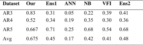
TABLE 4:COMPARISON OF CBC WITH ENS1,ANN,NB,VFI, AND ENS2 (AYSRE ET AL.2011), IN EMBEDDED DATASET ON PRECISION
Dataset Our Ens1 ANN NB VFI Ens2
AR3 0.83 0.31 0.05 0.22 0.39 0.41
AR4 0.52 0.34 0.19 0.35 0.30 0.36
AR5 0.667 0.71 0.25 0.68 0.54 0.68
Avg 0.675 0.45 0.17 0.42 0.41 0.48
Table 4shows the comparison of CBC with Ens1, ANN, NB, VFI, and Ens2 (Aysre et al. 2011) using precision. In precision Mann– Whitney tests: CBC is significant outperformed than Ens1 .Therefore we can conclude that our model is useful for the embedded systems and is performing better than the Ens1 consists of ANN, NB and VFI algorithms [23].Also our model is outperforming than the all constitute of Ens1(ANN,NB,VFI) and Ens2.
There is significant increase in precision rates from 45% in Ens1, 48% in Ens2 to 67.5% in our model.
Also it decreases false alarms by 13%, and hence increases precision by 22 %. From table 5 Mann–Whitney U tests show that the balance rates of two models are significantly different. Therefore we can conclude that our model is useful and is outperforming for the embedded systems.
TABLE 5:COMPARISON OF CBC WITH ENS1,ANN,NB,VFI, AND ENS2 (AYSRE ET AL.2011), IN EMBEDDED DATASET ON BALANCE
Dataset Our Ens1 ANN NB VFI Ens2
AR3 0.79 0.69 0.34 0.64 0.71 0.72
AR4 0.67 0.70 0.50 0.71 0.66 0.70
AR5 0.898 0.81 0.53 0.80 0.82 0.81
We validated the performance of CBC on embedded datasets to compare with both Ens1 and En2 the model of Ayse et al. (20011). From Table 3,4, and 5, it is easily seen that the CBC significantly improve false alarms, precision and balance rates for embedded system fault prediction. As from result Tables, Ens1 produces (76%, 22%, 45%, 73%) in terms of (pd, pf, prec, bal) on embedded datasets, whereas our CBC approach produced (76%, 9%, 67%, 79%) respectively which in term significantly reduces false alarms by 13% from Ens1 and 8 % from Ens2 .It also increases the precision by 19% from Ens1 and 18% from Ens2. Therefore, CBC is much better for embedded system software in terms of the confidence (precision) and false alarm of predictions.
VI.CONCLUSIONS
We presented a CBC method and process for software fault prediction. We have conducted several experiments in order to compare the performances of our model. The effectiveness of the method is demonstrated using several embedded dataset from promise repository. We employed statistical methods to assess the validity of our results; we have conducted the Mann–Whitney U test to evaluate whether the changes in pf, precision and balance can be significantly validated. Statistical tests prove the validity of our results in terms of false alarms, precision and balance. We conclude that discretization on software defect data with Fayyad & Irani’s [36] supervised discretization should be preferred and CBC approach perform better than Ens1or Ens2 [23]. The time complexity of ensemble methods, increases rapidly with dimensionality of the data and is constructed by constitution of various algorithms. But our method uses a single CBC technique and is also good for huge data. From a software practitioner’s point of view, these results are useful for detecting faults before proceeding to the test phase. In this sense, test resources can be managed more efficiently. The contributions of this research are two folds: In empirical studies replications are very important to improve, refute, and validate the results of others [5, 45]. Ayse et al. donated data to the promise repository which is publicly available to encourage other researchers to repeat, improve or refute their study; our work is the first response to their call. This research is not only a replication study, but also provides an effective software fault predictor model for embedded dataset.
On all projects, our model detects 76% defective modules while producing 9% false alarms. Our model significantly improves the precision from 48% to 67%.It also manages to improve the balance rates from 74% to 79% on average (all projects). Furthermore we will attempt to use intelligent computing for data preprocessing or activities for the removal of non informative features to improve the performance of software fault prediction models.
REFERENCES
[1] M.J. Harrold, Testing: a roadmap, in: Proceedings of the
Conference on the Future of Software Engineering, ACM Press, New York, NY, 2000.
[2] B.V. Tahat, B. Korel, A. Bader, “Requirement-based automated
black-box test generation” in: Proceedings of the 25th Annual
International Computer Software and Applications Conference, Chicago, Illinois, 2001, pp. 489–495
[3] Wohlin, C., Aurum, A., Petersson, H., Shull, F., & Ciolkowski, M.
(2002). “Software inspection benchmarking— A qualitative and quantitative comparative opportunity”. In METRICS ’02: Proceedings of the 8th international symposium on software metrics (pp. 118–127). IEEE Computer Society.
[4] Basili, V. R., Briand, L. C., & Melo, W. L. (1996). A validation of
object-oriented design metrics as quality indicators. IEEE Transactions on Software Engineering. IEEE Press, 22, 751–761
[5] Menzies, T., Greenwald, J., & Frank, A. (2007). Data mining static
code attributes to learn defect predictors. IEEE Transactions on Software Engineering, IEEE Computer Society, 32(11), 2–13
[6] F. Shull, V.B. Boehm, A. Brown, P. Costa, M. Lindvall, D. Port, I.
Rus, R. Tesoriero, and M. Zelkowitz, “What We Have Learned About Fighting Defects,” Proc. Eighth Int’l Software Metrics Symp., pp. 249-258, 2002
[7] Tosun, A., Turhan, B., & Bener, A. (2009).” Practical
Considerations in Deploying AI for defect prediction: A case study within the Turkish telecommunication industry”. In PROMISE’09: Proceedings of the first international conference on predictor models in software engineering. Vancouver, Canada.
[8] N. Nagappan and T. Ball, “Static Analysis Tools as Early Indicators
of Pre-Release Defect Density”, Proc. Intl Conf. Software Eng., 2005.
[9] T. Khoshgoftaar and E. Allen, “Model Software Quality with
Classification Trees,” Recent Advances in Reliability and Quality Eng., pp. 247-270, 2001.
[10] Li, Q., & Yao, C. (2003). Real-time concepts for embedded systems.
San Francisco: CMP Books.
[11] M. Evett, T. Khoshgoftaar, P. Chien, E. Allen, “GP-based software
quality prediction”, in: Proceedings of the Third Annual Genetic Programming Conference, San Francisco, CA, 1998, pp. 60–65.
[12] T.M. Khoshgoftaar, N. Seliya, “Software quality classification
modeling using the SPRINT decision tree algorithm”, in: Proceedings of the Fourth IEEE International Conference on Tools with Artificial Intelligence, Washington, DC, 2002, pp. 365–374.
[13] M.M. Thwin, T. Quah, “Application of neural networks for software
quality prediction using object-oriented metrics”, in: Proceedings of the 19th International Conference on Software Maintenance, Amsterdam, The Netherlands, 2003, pp. 113–122.
[14] K. El Emam, S. Benlarbi, N. Goel, S. Rai, “Comparing case-based
reasoning classifiers for predicting high risk software components”, Journal of Systems and Software 55 (3) (2001) 301–320.
[15] X. Yuan, T.M. Khoshgoftaar, E.B. Allen, K. Ganesan, “An
application of fuzzy clustering to software quality prediction”, in: Proceedings of the Third IEEE Symposium on Application-Specific Systems and Software Engineering Technology, IEEE Computer Society, Washington, DC, 2000, pp. 85.
[16] H.M. Olague, S. Gholston, S. Quattlebaum, “Empirical validation of
three software metrics suites to predict fault-proneness of object-oriented classes developed using highly iterative or agile software development processes”, IEEE Transactions on Software Engineering 33 (6) (2007) 402–419.
[17] K.O. Elish, M.O. Elish, “Predicting defect-prone software modules
using support vector machines”, Journal of Systems and Software 81 (5) (2008) 649–660.
[18] Catal C, Diri B. ”Investigating the effect of dataset size, metrics sets,
and feature selection techniques on software fault prediction problem”, Information Sciences. 179:pp.1040-1058,2009.
[19] P. Tomaszewski, J. Hakansson, H. Grahn, and L. Lundberg,
“Statistical models vs. expert estimation for fault prediction in modified code-an industrial case study”, The Journal of Systems and Software, vol. 80, no. 8, pp. 12271238, 2007.
[20] I. Gondra, “Applying learning to software fault machine -proneness
prediction”, Journal of Systems and Software 81 (2) (2008) 186– 195.
[21] T. Quah, “Estimating software readiness using predictive models”,
Information Sciences, 2008
[22] B. Turhan and A. Bener, Analysis of Naive Bayes Assumptions on
Software Fault Data: An Empirical Study, Data & Knowledge Eng., vol. 68, no. 2, pp. 278-290, 2009.
[23] Ayse Tosun Misirli, Ayse Basar Bener, Burak Turhan: “An
[24] Boetticher, G., Menzies, T., & Ostrand, T. J. (2007). “The PROMISE repository of empirical software engineering data “West Virginia University, Lane Department of Computer Science and Electrical Engineering.
[25] http://promise.site.uottowa.ca/SERepository
[26] Amasaki, S., Takagi, Y., Mizuno, O., & Kikuno, T. (2005).
“Constructing a Bayesian belief network to predict final quality in embedded system development.” IEICE Transactions on Information and Systems, 134, 1134–1141.
[27] Kan, S. H. (2002). Metrics and models in software quality
engineering. Reading: Addison-Wesley.
[28] Oral, A. D., & Bener, A. (2007). “Defect Prediction for Embedded
Software”. ISCIS ’07: Proceedings of the 22nd international symposium on computer and information sciences (pp. 1–6).
[29] T.M. Khoshgoftaar, N. Seliya, “Fault prediction modeling for
software quality estimation: comparing commonly used techniques”, Empirical Software Engineering 8 (3) (2003) 255–283
[30] Zhong, S., Khoshgoftaar, T.M., and Seliya, N., “Analyzing
Software Measurement Data with Clustering Techniques”, IEEE Intelligent Systems, Special issue on Data and Information Cleaning and Pre-processing, Vol (2), 2004, pp. 20-27.
[31] T. Menzies, J. DiStefano, A. Orrego, and R. Chapman, “Assessing
Predictors of Software Defects,” Proc. Workshop Predictive Software Models, 2004.
[32] Fenton, N., Neil, M., “A Critique of Software Defect Prediction
Models”, IEEE Transactions on Software Engineering, Vol 25(5), 1999, pp.675-689.
[33] M. Halstead, Elements of Software Science. Elsevier, 1977.
[34] T. McCabe, “A Complexity Measure,” IEEE Trans. Software
Eng.,vol. 2, no. 4, pp. 308-320, Dec. 1976.
[35] S. Lessmann, B. Baesens, C. Mues, and S. Pietsch. “Benchmarking
classification models for software fault prediction”: A proposed framework and novel findings. IEEE Transactions on Software Engineering, 2008.
[36] U. M. Fayyad and K. B. Irani,” Multi-interval discretisation of
continuous-valued attributes," in Proceedings of the Thirteenth International Joint Conference on Artificial Intelligence. 1993, pp. 1022-1027,
[37] D. Chiu, A. Wong, and B. Cheung, “Information Discovery through
Hierarchical Maximum Entropy Discretization and Synthesis,” Knowledge Discovery in Databases, G. Piatesky-Shapiro and W.J. Frowley, ed., MIT Press, 1991.
[38] X. Wu, “A Bayesian Discretizer for Real-Valued Attributes,” The
Computer J., vol. 39, 1996.
[39] A. Paterson and T.B. Niblett, ACLS Manual. Edinburgh: Intelligent
Terminals, Ltd, 1987
[40] R. Kerber, “ChiMerge: Discretization of Numeric Attributes,” Proc.
Ninth Int’l Conf. Artificial Intelligence (AAAI-91), pp. 123-128, 1992.
[41] H. Liu and R. Setiono, “Feature Selection via Discretization,” IEEE
Trans. Knowledge and Data Eng., vol. 9, no. 4, pp. 642-645, July/ Aug. 1997.
[42] Dougherty, J., Kohavi, R., and Sahami, M. (1995), “Supervised and
Unsupervised discretization of continuous features”. Machine Learning 10(1), 57-78.
[43] Shull, F. J., Carver, J. C., Vegas, S., & Juristo, N. (2008). The role of replications in empirical software engineering. Empirical Software Engineering Journal, 13, 211–218.
[44] Hall, M. A., & Holmes, G. (2003). “Benchmarking attribute
selection techniques for discrete class data mining” IEEE transactions on knowledge and data engineering. IEEE Educational Activities Department, 15, 1437–1447.
[45] J. Lung, J. Aranda, S.M. Easterbrook, G.V. Wilson, “On the
difficulty of replicating human subjects studies in software engineering”, in: Proceedings of the 30th International Conference on Software Engineering, 2008, pp. 191–200.
[46] P. Singh and S. Verma, “An investigation of the effect of
discretization on defect prediction using static measures”, in Advances in Computing, Control, Telecommunication Technologies, ACT 09. International Conf on, 2009, pp. 837- 839.
[47] J. MacQueen. “Some methods for classification and analysis of
multivariate observations”. In Proc. 5th Berkeley Symp. Math. Statistics and Probability, pages 281-297, 1967.
[48] Lee, E. A. (2002). Embedded software, advances in computers