© 2017, IRJET | Impact Factor value: 6.171 | ISO 9001:2008 Certified Journal | Page 1810
DATA MINING APRIORI ALGORITHM IMPLEMENTATION USING R
D Kalpana
Assistant Professor, Dept. Of Computer Science and Engineering, Vivekananda Institute of Technology and Science,
Telangana, India
---***---Abstract –
R Data mining focuses mainly on learningmethods and steps in performing data mining using R Programming Language as a platform, and R ia an Open source tool, data mining using R is very interesting for learners at all levels. Data mining is the process of deciphering meaningful insights from existing Databases and analyzing results. In this paper I would like to explain how the data mining Apriori algorithm is implemented using R Programming, and also I have given briefing about the association rules.
Key Words: R, Data mining, Apriori, Association rule, support, confidence
1. INTRODUCTION
R is an open source programming language and software platform that provides statistical computing and visualization capabilities. Initial development was done by
Ross Ihaka and Robert Gentleman and currently it is developed by the R core team. R has established a reputation as an important tool for statistical modeling, data visualization, data mining and machine learning. The R language incorporates all of the standard statistical tests, models, graphics and analyses, as well as providing a comprehensive language for managing and manipulating data. Leading researchers in data science are widely using R in academia and software development. R is a GNU project which can be considered as a different implementation of S.
1.1 Essentials of R Programming
Understand and practice this section thoroughly. This is the building block of R programming knowledge. If we get this right, we would face less trouble in debugging. R has five basic or ‘atomic’ classes of objects. Wait, what is an object ?Everything we see or create in R is an object. A vector, matrix, data frame, even a variable is an object. R treats it that way. So, R has 5 basic classes of objects. This includes: Character
1. Numeric (Real Numbers) 2. Integer (Whole Numbers) 3. Complex
4. Logical (True / False)
Since these classes are self-explanatory by names, I wouldn’t elaborate on that. These classes have attributes. Think of attributes as their ‘identifier’, a name or number which aptly identifies them. An object can have following attributes:
1. names, dimension names 2. dimensions
3. class 4. length
Attributes of an object can be accessed using attributes()
function. The most basic object in R is known as vector. we can create an empty vector using vector(). Remember, a vector contains object of same class.
1.2 Advantages
1. R is open source and freely available software. 2. R implement a wide variety of statistical and
graphical techniques including classical statistical tests, linear and nonlinear modeling, time-series analysis, classification, clustering, and others. 3. R provides a very wide variety of graphics for
visualizing data. These capabilities are found in the base language and in specialized packages like ggplot2, vcd and scatterplot3d.
4. R has a large number of packages that virtually support any statistical technique and the R community is noted for its active contributions in terms of packages.
5. R is able to consume data from multiple systems like Excel, SPSS, Stata, SAS and relational databases 6. R runs on mostly used operating systems like Windows, Linux, and Mac OS. It is also supported on 32 and 64 bit systems.
7. R has a vibrant community that offers support and commercial support is also available.
8. R has stronger object-oriented programming facilities than most statistical computing languages which is inherited from S. Extending R is also eased by its lexical scoping rules.
1.3 Disadvantages
1. R is difficult to learn for users without any computer programming background
2. The documentation of R may be difficult to understand for a person without a good statistical training.
© 2017, IRJET | Impact Factor value: 6.171 | ISO 9001:2008 Certified Journal | Page 1811 there are some packages that can remedy this by
storing data on hard drive.
4. Some packages have a quality deficiency. However if a package is useful to many people, it will quickly evolve into a very robust product through collaborative efforts.
5. R lacks in speed and efficiency due to its design principles that are outdate
2. FUNCTIONALITY OF DATA MINING
Data mining is the process of extracting data from databases and data warehouses. Short stories or tales always help us in understanding a concept better but this is a true story, Wal-Mart’s beer diaper parable. A sales person from Wal-Mart tried to increase the sales of the store by bundling the products together and giving discounts on them. He bundled bread and jam which made it easy for a customer to find them together. Furthermore, customers could buy them together because of the discount.
To find some more opportunities and more such products that can be tied together, the sales guy analyzed all sales records. What he found was intriguing. Many customers who purchased diapers also bought beers. The two products are obviously unrelated, so he decided to dig deeper. He found that raising kids is grueling. And to relieve stress, parents imprudently decided to buy beer. He paired diapers with beers and the sales escalated. This is a perfect example of Association Rules in data mining.
This gives a beginner's level explanation of Apriori algorithm in data mining. And also we look at the definition of association rules. Let’s begin by understanding what Apriori algorithm is and why is it important to learn it.
2.1 Apriori Algorithm
Apriori is an algorithm for frequent item set mining and association rule learning over transactional databases. It proceeds by identifying the frequent individual items in the database and extending them to larger and larger item sets as long as those item sets appear sufficiently often in the database. It is very important for effective Market Basket Analysis and it helps the customers in purchasing their items with more ease which increases the sales of the markets. It has also been used in the field of healthcare for the detection of adverse drug reactions.
2.2 Association Rules
An association rule is of the form X => Y, where X = {x1, x2, ...,
xn}, and Y = {y1, y2,..., ym} are sets of items, with xi and yj being
distinct items for all i and all j. This association states that if a customer buys X, he or she is also likely to buy Y. In general, any association rule has the form LHS (left-hand side) => RHS (right-hand side), where LHS and RHS are sets
of items. The set LHS ∪ RHS is called an itemset, the set of items purchased by customers. For an association rule to be of interest to a data miner, the rule should satisfy some interest measure.
Two common interest measures are support and confidence. A rule can be defined as an implication, XY where X and Y are subsets of I(X,Y⊆I) and they have no element in common, i.e., X ⋂Y. X and Yare the antecedent and the consequent of the rule, respectively.
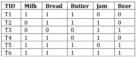
[image:2.595.323.544.368.464.2]Let’s take an easy example from the supermarket sphere. The example that we are considering is quite small and in practical situations, datasets contain millions or billions of transactions. The set of itemsets, I ={Milk, Bread, Butter, Jam, Beer} and a database consisting of six transactions. Each transaction is a tuple of 0's and 1's where 0 represents the absence of an item and 1 the presence. An example for a rule in this scenario would be {Milk, Bread} => {Butter}, which means that if milk and bread are bought, customers also buy a butter.
Table 1: Transactional Table
TID Milk Bread Butter Jam Beer
T1 1 1 1 0 0
T2 0 1 1 1 0
T3 0 0 0 1 1
T4 1 1 0 1 0
T5 1 1 1 0 1
T6 1 1 1 1 1
1) Support
The support of an itemset X, supp(X) is the proportion of transaction in the database in which the item X appears. It signifies the popularity of an itemset.
Supp(X) = No of Transaction in which X appears /Total no of transactions
In the example above, Supp(Milk)=4/6=0.66667
If the sales of a particular product (item) above a certain proportion have a meaningful effect on profits, that proportion can be considered as the support threshold. Furthermore, we can identify itemsets that have support values beyond this threshold as significant itemsets.
2) Confidence
Confidence of a rule is defined as follows:
Conf (XY)= supp (X U Y) / supp(X)
© 2017, IRJET | Impact Factor value: 6.171 | ISO 9001:2008 Certified Journal | Page 1812 probability of finding the itemset Y in transactions given the
transaction already contains X.
It can give some important insights, but it also has a major drawback. It only takes into account the popularity of the itemset X and not the popularity of . If Y is equally popular as X then there will be a higher probability that a transaction containing X will also contain Y thus increasing the confidence.
To overcome this drawback there is another measure called lift.
3) Lift
The lift of a rule is defined as:
lift (XY) = supp(X U Y) / supp(X) * supp(Y)
This signifies the likelihood of the itemset Y being purchased when item X is purchased while taking into account the popularity of Y.In this example above,If the value of lift is greater than 1, it means that the itemset Y is likely to be bought with itemset X, while a value less than 1 implies that itemset Y is unlikely to be bought if the itemset X is bought.
4) Conviction
The conviction of a rule can be defined as:
Conv(XY)= 1-supp(Y) / 1-conf(XY)
For the rule {milk, bread}=>{butter},The conviction value of 1.32 means that the rule {milk,bread}=>{butter} would be incorrect 32% more often if the association between X and Y was an accidental chance.
2.3 Working of Apriori Algorithm.
So far, we learned what the Apriori algorithm is and why is important to learn it.A key concept in Apriori algorithm is the anti-monotonicity of the support measure. It assumes that
1. All subsets of a frequent itemset must be frequent 2. Similarly, for any infrequent itemset, all its
supersets must be infrequent too
Let us now look at the intuitive explanation of the algorithm with the help of the example we used above. Before beginning the process, let us set the support threshold to 50%, i.e. only those items are significant for which support is more than 50%.
Step 1: Create a frequency table of all the items that occur in all the transactions. For our case:
Table2: Frequency table
Item Frequency Milk(M) 4 Bread(B) 5 Butter(Bu) 4
Jam(J) 4
Beer(Be) 2
Step 2: We know that only those elements are significant for which the support is greater than or equal to the threshold support. Here, support threshold is 50%, hence only those items are significant which occur in more than three transactions and such items are Milk, Bread, Butter and Jam. Therefore, we are left with:
Table3: Frequency Table with Minimum Support Item Frequency
Milk(M) 4
Bread(B) 5 Butter(Bu) 4
Jam(J) 4
The table above represents the single items that are purchased by the customers frequently.
Supp(X)=Number Of Transactions that in which X appears / Total number of Transactions
Step 3: The next step is to make all the possible pairs of the significant items keeping in mind that the order doesn’t matter, i.e., AB is same as BA. To do this, take the first item and pair it with all the others such as MB, MBu, MJ. Similarly, consider the second item and pair it with preceding items, i.e., BBu, BJ. We are only considering the preceding items because MB (same as BM) already exists. So, all the pairs in our example are. MB, MBu, MJ,BBu,BJ and BuJ.
Step 4: We will now count the occurrences of each pair in all the transactions.
[image:3.595.388.480.494.591.2]Step 5: Again only those itemsets are significant which cross the support threshold, and those are MB, MBu, BBu, and BJ
Table 4: Frequency table with 2-Itemset
Item Frequency
MB 4
Mbu 3
MJ 2
MB 4
BJ 3
BuJ 2
Step 6: Now let’s say we would like to look for a set of three items that are purchased together. We will use the itemsets found in step 5 and create a set of 3 items.
To create a set of 3 items another rule, called self-join is required. It says that from the item pairs MB, MBu, BBu, and BJ .we look for two pairs with the identical first letter and so we get
MB, MBu , this gives MBBu
BBu and BJ, this gives BBuJ
© 2017, IRJET | Impact Factor value: 6.171 | ISO 9001:2008 Certified Journal | Page 1813 Table 5: Frequency Table of 3-itemset
Itemset Frequency
MBBu 4 BBuJ 3
Applying the threshold rule again, we find that MBBu is the only significant itemset that satisfies minimum support Threshold. Therefore, the set of 3 items that was purchased most frequently is MBBu i.e Milk, Bread Butter.
The example that we considered was a fairly simple one and mining the frequent itemsets stopped at 3 items but in practice, there are dozens of items and this process could continue to many items. Suppose we got the significant sets with 3 items as MBBu and BBuJ now we want to generate the set of 4 items. For this, we will look at the sets which have first two alphabets common, i.e,MBBu and BBuj gives MBBuJ. In general, we have to look for sets which only differ in their last letter/item.Now that we have looked at an example of the functionality of Apriori Algorithm, let us formulate the general process.
2.4 General Process:
The entire algorithm can be divided into two steps:
Step 1: Apply minimum support to find all the frequent sets with k items in a database.
Step 2: Use the self-join rule to find the frequent sets with k+1 items with the help of frequent k-itemsets. Repeat this process from k=1 to the point when we are unable to apply the self-join rule.
This approach of extending a frequent itemset one at a time is called the “bottom up” approach.
Flowchart 1: Apriori Process
2.3.1 Mining Association Rules
Till now, we have looked at the Apriori algorithm with respect to frequent itemset generation. There is another task for which we can use this algorithm, i.e., finding association rules efficiently. For finding association rules, we need to find all rules having support greater than the threshold support and confidence greater than the threshold confidence. But, how do we find these? One possible way is brute force, i.e., to list all the possible association rules and calculate the support and confidence for each rule. Then eliminate the rules that fail the threshold support and confidence. But it is computationally very heavy and prohibitive as the number of all the possible association rules increase exponentially with the number of items. Given there are n items in the set I, the total number of possible association rules is .
We can also use another way, which is called the two-step approach, to find the efficient association rules.
The two-step approach is:
Step 1:Frequent itemset generation: Find all itemsets for which the support is greater than the threshold support following the process we have already seen earlier in this article.
Step 2:Rule generation: Create rules from each frequent itemset using the binary partition of frequent itemsets and look for the ones with high confidence. These rules are called candidate rules.
Let us look at our previous example to get an efficient association rule. We found that MBBu was the frequent itemset. So for this problem, step 1 is already done. So, let’ see step 2. All the possible rules using OPB are:
MB Bu, MBu B, BBu M, Bu MB, B MBu, M BBu
If X is a frequent itemset with k elements, then there are candidate association rules.
3.R IMPLEMENTATION
The package which is used to implement the Apriori algorithm in R is called arules. The function that we will demonstrate here which can be used for mining association rules is
apriori(data, parameter = NULL)
The arguments of the function apriori are
data: The data structure which can be coerced into transactions (e.g., a binary matrix or data.frame).
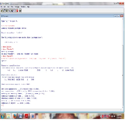
© 2017, IRJET | Impact Factor value: 6.171 | ISO 9001:2008 Certified Journal | Page 1814 run R Programming, We have to install R programming and
[image:5.595.36.285.176.416.2]it supports all operating systems. It is a open source software.No need to pay any subscription charges. Availability of instant access to over 7800 packages customized for various computation tasks
.
Fig 1: R Gui Console
After Applying arules for Adult dataset the result will be given as
> library(arules) > data("Adult")
> rules <- apriori(Adult,parameter = list(supp = 0.5, conf = 0.9, target = "rules"))
> summary(rules)
#set of 52 rules
#rule length distribution (lhs + rhs):sizes # 1 2 3 4
# 2 13 24 13
# Min. 1st Qu. Median Mean 3rd Qu. Max. # 1.000 2.000 3.000 2.923 3.250 4.000
# summary of quality measures: # support confidence lift
# Min. :0.5084 Min. :0.9031 Min. :0.9844 # 1st Qu.:0.5415 1st Qu.:0.9155 1st Qu.:0.9937
# Median :0.5974 Median :0.9229 Median :0.9997 # Mean :0.6436 Mean :0.9308 Mean :1.0036 # 3rd Qu.:0.7426 3rd Qu.:0.9494 3rd Qu.:1.0057 # Max. :0.9533 Max. :0.9583 Max. :1.0586
# mining info:
# data ntransactions support confidence # Adult 48842 0.5 0.9
> inspect(rules) #It gives the list of all significant association rules. Some of them are shown below
# lhs rhs support confidence lift
# [1] {} => {capital-gain=None} 0.9173867 0.9173867 1.0000000
# [2] {} => {capital-loss=None} 0.9532779 0.9532779 1.0000000
# [3] {hours-per-week=Full-time} => {capital-gain=None} 0.5435895 0.9290688 1.0127342
# [4] {hours-per-week=Full-time} => {capital-loss=None} 0.5606650 0.9582531 1.0052191
# [5] {sex=Male} => {capital-gain=None} 0.6050735 0.9051455 0.9866565
# [6] {sex=Male} => {capital-loss=None} 0.6331027 0.9470750 0.9934931
# [7] {workclass=Private} => {capital-gain=None} 0.6413742 0.9239073 1.0071078
# [8] {workclass=Private} => {capital-loss=None} 0.6639982 0.9564974 1.0033773
# [9] {race=White} => {native-country=United-States} 0.7881127 0.9217231 1.0270761
# [10] {race=White} => {capital-gain=None} 0.7817862 0.9143240 0.9966616
4. CONCLUSIONS
© 2017, IRJET | Impact Factor value: 6.171 | ISO 9001:2008 Certified Journal | Page 1815
REFERENCES
[1] M. Young, The Technical Writer’s Handbook. Mill Valley,
CA: University Science, 1989.
[2] Hornik, Kurt (November 26, 2015). "R FAQ". The
Comprehensive R Archive Network. 2.1 What is R ? Retrieved 2015-12-06.
[3] David Smith (2012); R Tops Data Mining Software Poll,
Java Developers Journal, May 31, 2012.K. Elissa, “Title of paper if known,” unpublished.
[4] S. van Buuren and K. Groothuis-Oudshoorn. MICE: