ISSN 2348 – 7968
493
Agent Based Markov Chain for Job Shop Scheduling and
Control: Review of the Modeling Technigue.
Chiagunye Tochukwu1, Inyiama Hyacinth2, Nwachukwu‐nwokeafor K.C1
Computer Engineering Dept. Michael Okpara University of Agriculture, Umudike, Abia State Nigeria.1
Electronic and Computer Engr. Dept. Nnamdi Azikiwe Unuversity Awka, Anambra State Nigeria.2
ABSTRACT
Owing to its impact on the industrial economy, the job shop scheduler and controller are vital algorithms for modern manufacturing processes. This paper is concerned with the review of the modeling of agent based markov chain for job shop scheduling and control. The work adopts an alternative view on job-shop scheduling problem where each resource is equipped with adaptive agent that, independent of other
agents makes job dispatching decision based on its local view of the plant. Given the fact that agent based
modeling is proven to be an effective way of modeling complex systems that are not easy to characterize analytically, this work is focused on addressing the JSP by developing an agent based model in which all information of the dynamics of the model is formulated as a Markov chain.
Keywords; Agent, Job shop, Scheduling, Makespan, algorithm, Markov Chain
1.0 Introduction
The urgent need for high responsiveness and flexibility in coping with the dynamic market changes has been demonstrated by the study carried out by Zhang and Sharifi (2001) [1] involving a case with 12 companies and a questionnaire survey with 1000 companies. The analysis of the study also indicates that, in order to achieve high responsiveness, one of the operational issues to be focused on is production planning and control, particularly process planning and production scheduling, which must be dynamically and cost-effectively integrated. However, the conventional control strategies for manufacturing systems were not designed to achieve such responsiveness.
In the United States alone, there are over 40,000 factories producing metal-fabricated parts [2]. These parts end up in a wide variety of products sold in the US and elsewhere. These factories employ roughly over 3 million people and ship close to $ 7 billion worth of products every year. The vast majority of these factories are what is called “job shops”, meaning that the flow of raw and unfinished goods through them is completely random. Over the years, the behavior and performance of these job shops have been the focus of considerable attention in the Operations Research (OR) literature.
ISSN 2348 – 7968
is concerned with the problem of assigning a set of jobs to resources over a period of time. Effective scheduling plays a very important role in today’s competitive manufacturing environment. Performance Criteria such as machine utilization, manufacturing lead times, inventory costs, meeting due dates, customer satisfaction, and quality of products are all dependent on how efficiently the jobs are scheduled in the system [6]. Hence, it becomes increasingly important to develop effective scheduling approaches that help in achieving the desired objectives.
The scheduling and planning of production order have an important role in the manufacturing system. The diversity of products, increased number of orders, the increased number and size of workshops and expansion of factories have made the issue of scheduling production orders more complicated, hence the traditional methods of optimization are unable to solve them [7][8].
With respect to related studies, [9] proposed a methodology for solving the job shop problem based on the decomposition of mathematical programming problems that used both Benders-type [10] and Dantzig/wolfe-type [11] decompositions. The methodology was part of closed loop, real-time, two-level hierarchical shop floor control system. The top-level scheduler (i.e., the supremal) specified the earliest start time and the latest finish time for each job. The lower level scheduling modules (i.e., the infimals) would refine these limit times for each job by detailed sequencing of all operations. A multi-criteria objective function was specified to include tardiness, throughput, and process utilization cost. The limitations of this methodology stem from the inherent stochastic nature of job shops and the presence of multiple, but often conflicting, objectives made it difficult to express the coupling constraints using exact mathematical relationships. This made the schedule not to converge. Furthermore the rigid centralization of the scheduler made it not able to adjust to disturbances at the shop floor. [12] evaluated the use of MRP or MRP-11 to create a medium-range scheduler. MRP system’s major disadvantages are rigidity and the lack of feedback from the shop floor, but also the tremendous amount of data that have to be entered in the bill of materials and the fact that the model of the manufacturing system and its capacity are excessively simple.
As can be deduced from these techniques, most approaches to job-shop scheduling assume complete task knowledge and search for a centralized solution. These techniques typically do not scale with problems size, suffering from an exponential increase in computation time. The centralized view of the plant coupled with the deterministic algorithms characteristic of these schedulers do not allow the manufacturing processes to adjust the schedule (using local knowledge) to accommodate disturbances such as machine breakdowns. Hence a production scheduling and control that performs reactive (not deterministic) scheduling and can make decision on which job to process next based solely on its partial (not central) view of the point becomes necessary. This requirement puts the problem in the class of agent based model (ABM). Hence this work adopts an alternative view on job-shop scheduling problem where each resource is equipped with adaptive agent that, independent of other agents makes job dispatching decision based on its local view of the plant.
1.1 Statement of the Problem
This work explore the well known n x m static Job Scheduling Problem (JSP) [13] in which n jobs must
be processed exactly once on each of m machines. Each job i (1 i n) is routed through each of the m
machines in a predefined order i, where i(j) denotes the jth machine (1 ʲ m) in the routing order.
The processing of job ¡ on machine i(ʲ) is denoted Oij and is called an operation. An operation Oij
must be processed on machine i(ʲ) for an integral duration Tij О. The scheduling objective is
ISSN 2348 – 7968
495
As indicated in the introduction of this work, the existing deterministic shop floor schedulers do not
possess the capability that allow the dispatch of Oij to react to disturbances on the factory floor, such as
break down of i(ʲ), arrival of new job i, all which require frequent re-planning that introduces
complexities (making the JSP N-P hard). Also given the fact that agent based modeling (ABM) is proven to be an effective way of modeling complex systems that are not easy to characterize analytically, this paper is focused on addressing the JSP by developing an agent based model in which all information of the dynamics of the model is formulated as a markov chain.
1.2 Significance of the Study
Efficient shop floor scheduling is very vital in a production system that relies heavily on the tight integration of the upstream supplier of parts, the midstream manufacturer and assembler of components, and the downstream distributor of finished goods. The successful outcome of this work should be of great prospect to raising the performance of this sort of supply chain that relies heavily on the shop floor scheduling and control mechanism of the middle manufacturer.
Globalization and strong competition in the current market place have forced companies to change their ways of doing business. Manufacturers have been compelled to adopt strategies such as Build-to-order (BTO) or Configuration-Build-to-order (CTO) services. These all geared towards harnessing Just-in-Time (JIT) and Total Quality Management (TQM) strategies in order to realize greater plant productivity, improved processes and products, lower cost and higher profits. The methodical leverage of the contributions of this work would help remove the bottleneck currently inherent at the shop floor towards the effective exploitation of these production management strategies.
2.1 Job Shop Scheduling
Scheduling is an important tool for manufacturing and engineering, where it can have a major impact on the productivity of a process [14]. In manufacturing, the purpose of scheduling is to minimize the production time and cost, by telling a production facility when to make, with which staff, and on which machine.
Survey of the literature indicates that the job shop scheduling problem (or job-shop problem) is at least 70 years old. In the publications [15][16][17], job shop scheduling is reported as an optimization problem in computer engineering and operations research in which ideal jobs are assigned to resources at particular times. The most basic version is described [15] as follows:
Given n jobs J1, J2, …… Jn of varying sizes, which need to be scheduled on m identical machines, the
task is to work out the scheme for assigning job i to machine mi in order to minimize the makespan. The
makespan is the total length of the schedule (that is, when all the jobs have finished processing). In the literature nowadays, the problem is presented as an online problem (dynamic scheduling), that is, each job is presented, and the online algorithm needs to make a decision about that job before the next job is presented. This problem is one of the best known online problems, and was the first problem for which competitive analysis was presented, by Graham [18]. Best problem instances for basic model with make span objectives are due to Taillard [19].
ISSN 2348 – 7968
Exploration of the literature indicates the disjunctive graph [21] as one of the popular models used for describing the job shop scheduling problem (JSP) instances [22].
A mathematical statement of the problem can be as follows:
Let m = {M1, M2, ……Mm} and J= {J1, J2,……Jn} be two finite sets. On account of the industrial origins
of the problem, the Mi are called machines and the Jʲ are called jobs.
Let denote the set of all sequential assignments of jobs to machines, such that every job is done by
every machine exactly once; element ∈ may be written as n x m matrices, in which column i lists the
jobs
that machine Mi will do, in order. For example, the matrix
1 2 2 3 3 1
Means that machine M1 will do the three jobs J1, J2, J3, in the order J1, J2, J3, while machine M2 will do
the jobs in the order J2, J3, J1. Suppose also that there is some cost function ∁: → 0 ∞. The cost
function may be interpreted as a “total processing time”, and may have some expression in terms of time.
Cij: M x J → 0 ∞, the cost /time for machine Mi to do job Jʲ.
The job-shop problem is to find an assignment of jobs ∈ such that ∁ is a minimum, that is, there is
no ∈ such that ∁ ∁ .
The reference [15] noted that one of the first problems that must be dealt with in the JSP is that many
proposed solutions have infinite cost: i.e., there exists ∞∈ such that ∁ ∞ ∞. Infact, it is quite
simple to concoct examples of such ∞ by ensuring that two machines will deadlock, so that each waits
for the output of the other’s next step.
Graham had already provided the list scheduling algorithm, which is (2-1/m) – competitive, where m is the
number of machines [18]. Also, it was proved that list scheduling is optimum online algorithms for 2 and 3 machines. The Coffman – Graham algorithm [23] for uniform – length jobs is also optimum for two
machines, and is (2-2/
m) – competitive. Bartal et.al. [24] presented an algorithm that is 1.986 competitive.
It is reported [25] that a 1.945 – competitive algorithm was presented by Kanger, Philips and Torry. Albers [26] provided a different algorithm that is 1.923 – competitive. Currently, the best known result is an algorithm given by Fleischer and Wahl, which achieves a competitive ratio of 1.9201 [27].
2.3 Offline Makespan Minimization
ISSN 2348 – 7968
497 2.4 Job Consisting of Multiple Operations
The basic form of the problem of scheduling jobs with multiple (m) operations over m machines, such that all of the first operations must be done on the first machine, all of the second operations on the second, etc., and a single job cannot be performed in parallel, is known as the open shop scheduling problem. Various algorithms are reported [29] in the literature.
A heuristic algorithm by Johnson [30] can be used to solve the case of a 2 machine N job problem when all jobs are to be processed in the same order. The steps of the algorithm are as follows:
Job Pi has two operations, of duration Pi 1, Pi 2, to be done on machines M
1, M2 in that sequence.
Step 1. List A = {1,2, ….., N}, List L
1 = { }, List L2 = { }
Step 2, from all available operation durations, pick the minimum.
If the minimum belongs to Pk1,
remove K from list A; Add K to end of list L1 if minimum belongs to Pk2, remove K from list A; Add K
to beginning of list L2.
Step 3. Repeat step 2 until list A is empty
Step 4. Join list L1, list L2. This is the optimum sequence.
Johnson’s method only works optimally for two machines. However, since it is optimal, and easy to compute, some researchers have tried to adopt it for M machines, (m>2).
The idea is as follows: Imagine that each job requires m operations in sequence, on m1, m2, ….Mm, the
first m/
2 machines are combined into an (imaginary) machining center, MC1, and the remaining machines
into a machining center MC2. Then the total processing time for a job P on MC1 = Sum (operation times
on first m/
2 machines), and processing time for job P on MC2 = sum (operation times on last m/2 machines).
By doing so, the m – machine problem is said to be reduced to a two machining center scheduling problem. This can then be solved by using the Johnson’s method.
2.5 Markov Chain
A Markov Chain [31] named after Andrey Markov, is a mathematical system that undergoes transition from one state to another on a state space. A Mark Chain is a stochastic process with the Markov property. The term “Markov Chain” refers to the sequence of random variables such a process moves through, with the Markov property defining serial dependence only between adjacent periods (as in a “Chain”). It can thus be used for describing systems that follow Chain-of linked events, where what happens next depends only on the current state of the system. In the literature, different Markov processes are designated as “Markov Chains”. Usually however the term is reserved for a process with a discrete set of times (i.e. a discrete-time Markov Chain (DTMC) [32], although some authors use the same terminology to refer to a continuous – time Markov Chain without explicit mention [33][34]. While the time parameter definition is mostly agreed upon to mean discrete-time, the Markov Chain state space does not have an established definition: the term may refer to a process on an arbitrary general state space [35]. However, many uses of Markov Chain employ finite or countable (discrete on the real line) state space, which have a more straightforward statistical analysis.
2.6 Formal Definition
A Markov Chain is a sequence of random variable X1, X2, X3,…… with the Markov property, namely
ISSN 2348 – 7968
Pr (Xn+r = x/X1, = x1, X2 = x2 ….., Xn = xn) = Pr (Xn+r = x/Xn = xn), if both conditional probabilities are
defined, i.e.
if Pr (X1 = x1, ……, Xn = xn) >0 the possible values of Xi form a countable set S called the state space
of the Chain.
Markov Chains are often described by a sequence of directed graphs, where the edges of graph n are labeled by the probabilities of going from one state at time n to other states at time n+1,
Pr (Xn+1 = x/Xn = xn). The same information is represented by the transition matrix from time n to time
n+1. However, Markov Chains are frequently assumed to be time-homogenous, in which case the graph and matrix are independent of n and so are not presented as sequences.
These descriptions highlight the structure of the Markov Chain that is independent of the initial
distribution Pr (X1 = x1). When time-homogenous, the Chain can be interpreted as a state machine
assigning a probability of hopping from each vertex or state to an adjacent one. The probability Pr (Xn =
x/X1 = x1) of the machines state can be analyzed as the statistical behavior of the machine with an element
x1 of the state space as input, or as the behavior of the machine with the initial distribution Pr (X1 = y) =
[x1 = y] of states as input, where (P) is the /verson bracket. The stipulation that not all sequences of states
must have nonzero probability of occurring allows the graph to have multiple connected components, suppressing edges encoding a zero (O) transition probability, as if a has a nonzero probability of going to
b but a and x lie in different connected components, then Pr (Xn+1 = b/Xn = a) is defined, while Pr (Xn+1 =
b/X1 = x, …..xn = a) is not. [35]
Variations
Continuous –time Markov processes have a continuous index
Time-homogenous Markov Chains (or stationary Markov Chains) are processes where Pr (Xn+1 =
x/Xn = y) = Pr (Xn = x/Xn-1 = y) for all n. The probability of the transition is independent of n.
A Markov Chain of order m (or a Markov Chain with memory m), where m is finite, is a process
satisfying
Pr (Xn = xn/Xn-1 = xn-1, Xn+2 = xn-2, …….. X1 = x1)
= Pr (Xn = xn/Xn-1 = xn-1, Xn-2 = xn-2, …….. Xn-m = xn-m) for n > m 2.1
In other words, the future state depends on the past m states. It is possible to construct a Chain (Yn) from
(Xn) which has the ‘classical’ Markov property by taking as state space the ordered m – tuples of x values,
i.e. Yn = (Xn, Xn-1, ………, Xn-m+1).
Transient Evolution
The probability of going from state i to state j in n time steps is Pij(n) =Pr (Xn = j /X0 = i) 2.2
and the single – step transition is
Pij =Pr (X1 = j /X0 = i) 2.3
For a time-homogenous Markov Chain:
Pij(n) =Pr (Xk+n = j /Xk = i) 2.4
and
Pij =Pr (Xk+1 = j /Xk = i) 2.5
The n-step transition probabilities satisfy the Chapman –Kolmogrov equation, that for any K such that 0<k<n,
2.6
ISSN 2348 – 7968
499
where S is the state space of the Markov Chain.
The marginal distribution Pr (Xn = x) is the distribution over states at time n. The initial distribution is Pr
(X0=x). The evolution of the process through one time step is described by
2.7
Properties
A state j is said to be accessible from a state i (written i→j) if a system started in state has a non-zero
probability of transitioning into state j at some point. Formally, state j is accessible from state:
If there exists an integer nij≽0 such that
Pr (Xnij = j/X0 = i) = Pij(nij) > 0. 2.8
This integer is allowed to be different for each pair of states hence the subscripts in nij. Allowing n to be
zero means that every state is defined to be accessible from itself.
A state i is said to communicate with state j (written i↔j) if both i ⟶ j and j ⟶ i. A set of state (is a
communicating class if every pair of states in C communicates with each other, and no state in C communicates with any state not in C. It can be shown that communication in this sense is an equivalence relation and thus that communicating classes are the equivalent classes of this relation. A communicating class is closed if the probability of leaving the class is zero, namely that if i is not in j, then j is not accessible from i.
A state i is said to be essential or final if for all j such that i ⟶ j it is also true that j ⟶ i. A state i is
inessential if it is not essential [36].
A Markov Chain is said to be irreducible if its state space is a single communicating class, in other words, if it is possible to get to any state from any state.
Periodicity
A state i has period k if any return to state i must occur in multiple of k time steps. Formally, the period of a state is defined as:
K = gcd {n : Pr (Xn = i/X0 = i) 0}
(where “gcd” is the greatest common division). Note that even though a state has period k, it may not be possible to reach the state in k steps. For example, suppose it is possible to return to the state in {6,8,10,12….} time steps; k would be 2, even though 2 does not appear in this list.
If k = 1, then the state is said to be a periodic: returns to state i can occur at irregular times, in other
words, a state i is aperiodic if there exists n such that for all n1 ≽ ,
Pr (Xn1 = i /X0 = i) > 0
Otherwise (k>1), the state is said to be periodic with period k. a Markov Chain is aperiodic if every state is aperiodic. An irreducible Markov Chain only needs one aperiodic state to imply all states are aperiodic. Every state of a bi partite graph has an even period.
Recurrence
A state i is said to be transient if, given that the system start in state i, there is a non-zero probability that the system will never return to i formally, but the random variable Ti be the first return time to state i (the
P
r(X
n= j) = ∑
P
rʲP
r(X
n-1= r) = ∑
(n)P
rʲP
r(X
0= r)
∞
ISSN 2348 – 7968
“hitting time”): Ti = inf{n≽1:Xn = i /X0 = i} the number fii(n) = Pr (Ti = n) is the probability that state is
returned to for the first time after n steps. Therefore, state i is transient if
State i is recurrent (or persistent) if it is not transient. Recurrent states are guaranteed to have a finite hitting time.
Even if the hitting time is finite with probability 1, it need not have a finite expectation. The mean
recurrence time at state i is the expected return time Mi.
2.10
State i is positive recurrent (or non-null persistent) if Mi is finite; otherwise, state i is null recurrent (or
null persistent).
It can be shown that a state i is recurrent if and only if the expected number of visits to this state is infinite, i.e.
2.11
A state i is called absorbing if it is impossible to leave this state. Therefore, the state i is absorbing if and only if
Pii = 1 and Pij = 0 for i ‡ j
2.7 Agent-Based Modeling (ABM)
Agent-based modeling (ABM) is a modeling approach reported [37] to have gained increasing attention over the past 18 years or so. This growth trend is evidenced by the increasing number of applications, articles appearing in modeling and applications journals, funded programs that call for agent-based models incorporating elements of human and social behavior, the growing number of conferences on or that have tracks dedicated to agent-based Modeling, the demand for ABM courses and instructional programs, and the number of preparations at conferences such as the WSC that references agent-based Modeling. Some authors [38][39] contend that ABM “is a third way of doing science” and could augment traditional deductive and inductive reasoning as discovered methods.
Based on survey of the literature, it can be said that agent-based modeling is being applied to many areas, spanning human social, physical and biological systems. It is reported that applications range from modeling ancient civilizations that have been gone for hundreds of years, to designing new markets for products that do not exist right now. Heath et al [40] provides a review of agent-based modeling applications. Selected applications that use the Repast agent-based modeling toolkit are listed in table 2.1. All of the cited publications make the case for agent-based Modeling as the preferred modeling approach against other modeling techniques for the problem addressed. These cited publications (refer to table 2.1) argue that agent-based modeling is used because only agent-based model can explicitly incorporate the complexity arising from individual behaviors and interactions that exist in the real-world.
2.8 Designing Agent-Based Model
Modern software practices are based on a template design approach in which recurring elements are codified and reused for new applications; this approach has proven very valuable in designing model’s as
∞
Mi = £ [Ti] = ∑ .
fii
(n)n=1
∞
∑ Pii
(n)= ∞
ISSN 2348 – 7968
501
well as software. Several formats have been proposed for describing agent-based designs. Chief among these standards is Grimm et al’s “Overview, Design concepts, and Detail (ODD) protocol [56]. ODD describes models using a three-part approach: overview, concepts, and details. The model overview includes a statement of the model’s intent, a description of the main variables, and a discussion of the agent activities and timing. The design concepts include a discussion of the foundations of the model, and the details include the initial setup configuration, input value definitions, and description of any embedded models [56].
North et.al [57] discussed product design patterns for agent-based modeling. For example, design patterns that have proven themselves useful for agent-based modeling includes:
Scheduler scramble: The problem addressed is when two or more agents from the ABM pattern can
schedule events that occur during the same clock tick. Getting to execute first may be an advantage or disadvantage. How do you allow multiple agents to act during the same clock tick without giving a long-term advantage to any one agent?
Context and projection Hierarchy: The problem addressed is how to organize complex space into a
single unified form such that individual agents can simultaneously exist in multiple spaces and the spaces themselves can be seamlessly removed and added.
Strategy: The problem addressed is how to let clients invoke rules that may be defined long after the
clients are implemented? There are a set of rules that need to be dynamically selected while a program is running. There is a need to separate rule creation from rule activation.
Learning: The problem addressed is to how to model agents that adapt or learn. There is need for
agents to change their behavior over time based on their experiences.
2.8 Markov Chain Approach for Agent-Based Modeling
Sven et.al [58] analyzed the dynamics of agent based models from a Markovian perspective and derived explicit statements about the possibility of linking a microscopic agent model to the dynamical processes of macroscopic observables that are useful for a precise understanding of the model dynamics. These authors strongly argue that it is in this way the dynamics of collective variables may be studied, and a description of macro dynamics as emergent properties of micro dynamics, in particular during transient times, is possible. This work [58] is a contribution to interweaving two lines of research that have developed in almost separate ways: Markov Chains and agent-based models. The former represents the simplest form of a stochastic process while the later puts a strong emphasis on heterogeneity and social interactions.
The usefulness of the Markov Chain formalism in the analysis of more sophisticated ABM has been discussed by Izquierds [59], who looked at 10 well-known social simulation models by representing them as a time-homogeneous Markov Chain. Among these models are the schelling segregation model [60], the Axelrod model of cultural dynamics [61] and the sugar scape model from Epstein and Axtell [62]. The main idea of Izquierdo et al [59] is to consider all possible configurations of system as the state space of the Markov Chain. Despite the fact that all the information of the dynamics on the ABM is encoded in a Markov Chain, it is difficult to learn directly from this fact, due to the huge dimension of the configuration space and its corresponding Markov transition matrix. The work [59] mainly relies on numerical computations to estimate the stochastic transition on metrices of the models.
ISSN 2348 – 7968
configuration space the set of all possible combinations of attributes of the agent, i.e., = SN. This also
incorporates models where agents move on a lattice (e.g., in the sugarscape model) because we can treat the sites as “agents” and use an attribute to encode whether a site is occupied or not. The updating process of the attributes of the agents at each time step typically consists of two parts. First, a random choice of a subset of agents of agents is made according to some probability distribution w. Then the attributes of the agents are updated according to a rule, which depends on the subset of agents selected at this time. With this specification, ABM can be represented by a so-called random map representation which may be taken as an equivalent definition of a Markov Chain [63]. Hence, ABM are Markov
Chains on with a transition matrix P. for a class of ABM the transition probabilities P(x,y) can be
computed for any pair , N of agent configurations. The process (,P) is referred to as micro chain.
When performing simulations of an ABM the actual interest is not in all the dynamical details but rather in the behavior of variables at the macroscopic level (mean job completion time, mean waiting time, mean
tardiness, etc.). The formulation of an ABM as a Markov Chain (,ṕ) enables the development of a
mathematical framework for linking the Micro-description of an ABM to a Macro-description of interest. Namely from the Markov Chain perspective, the transition from the micro to the macro level is a
projection of the Markov Chain with state space onto a new state space X by means of a (protection)
map from to X. The meaning of the projection is to lump sets of Micro configuration in
according to the macro property of interest in such a way that, for each xєX, all the configurations of in
-1 (x) share the same property.
3.0 Summary of Related Literature
Scheduling understood to be an important tool for manufacturing and engineering has a major impact on productivity of a process [14]. In manufacturing, the purpose of scheduling is to minimize the production time and cost, by telling a production facility when to make with which staff, and on which machine. Cited publications argued that agent-based modeling is used because only agent-based model can explicitly incorporate the complexity arising from individual behavior and interactions that exist in the real-world. [58] contributed to interweaving Markov Chains and agent-based modeling. [59] worked on and represented 10 well-known simulation models as a time homogenous Markov Chain. The author’s main idea is the formulation of the system configuration as the state space of the Markov Chain.
ISSN 2348 – 7968
503
this work adopts an alternative view on job shop scheduling problem where each resource is equipped with adaptive agent that independent of other agents, makes job dispatching decision based on its local view of the plant.
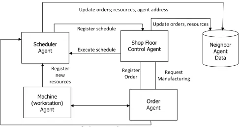
Fig.1: Block Diagram of the Proposed ABM Framework for Solving the JSP
Fig. 1 presents the shop for scheduler agent, shop floor control (SFC) agent, order agent and the machine (or work station) agent. This figure shows the interaction between the scheduler agent and other agents. First the agent needs a model of the surrounding agents. Agents have to register themselves with the SFC agent. Second, resources like a machine (or workstation) needs to notify the shop control agent when they have spear productivity capability. The order agent sends request for production capacity (to the scheduler agent or SFC agent), the function of the shop floor control agent is to match the request of the order agent with the offers of the resources on a certain instance of time. The SFC agent therefore uses the schedules it receives regularly from one or more schedules. Order agents and resources (or workstation) are not obliged to wait with their request and offers until the operation is executable or the resource is free. This enables the agents to foresee future events and consider the consequences of it. This will be used to have, e.g. an idle machine (workstation) waiting for an important order, even when work is available.
3.2 Analysis of the Existing System
Analysis of the integer programming formulation of the job shop scheduling problem is presented. In the integer programming technique, it is assumed that each job consists of m operations and most pass
Scheduler Agent
Machine (workstation)
Agent
Order Agent
Neighbor Agent
Data Shop Floor
Control Agent Update orders; resources, agent address
Update orders, resources
Execute schedule
Register schedule
Register
new
resources
Register
Order ManufacturingRequest
ISSN 2348 – 7968
through each machine exactly one. All machines are available at time zero. Furthermore, the total number of sublots is given and consistent sublot sizes are considered. In addition, transport times are negligible. With the notations and assumptions, the model can then be summarized as follows:
min Cmax 3.1
subject to:
= Di i 3.2
X
ij 0 i,j 3.3
δijk Xij i,j,k 3.4
tijk’ tijk + r
ik . δijk + Pik . Xij (0ijk, 0ijk
’)ЄA 3.5
ti (j+1)k tijk + r
ik . δijk + Pik . Xij i, k, j, < s 3.6
Cmak tisk + rik . δisk + Pik . Xis i, 0isk Є L 3.7
tijk ti’ j’ k + r
i’ k . δi’ j’ k + Pi’ k . Xi’ j’ - H . Yiji’ j’ k
ti’ j’ k tijk + r
ik . δijk + Pik . Xij - H . Yi’ ji’ j’ k
Yi ji’ j’ k +Yi’ j’ i j k = 1 i ‡i’, j, j’ 3.8 δi1k = 1 i, k 3.9
δi (j + 1)k Yi j i’ j’ k - Yi (j + 1) i’ j’ k
i ‡i’, j < s, j’ k 3.10
In this model the conventional make span objective function (3.1) is employed, constraint (3.2) ensure that all required units are produced. Constraints (3.3) are the non-negativity conditions. Since sublots sizes may equal 0, the actual number of sublots is possibly smaller than the given number S. This adds flexibility to the formulation with the fixed total number of sublot(s) obviously, no setup is necessary, if the corresponding sublot doesn’t exist. Constraints (3.4) are therefore used to avoid redundant setups. Constraints (3.5) represent the precedence relations of the operations that belong to the same sublot. When attached setup times are taken into consideration, the setup of a certain machine cannot begin until the corresponding sublot has been transferred to this machine. Constraint (3.5) fulfill this requirement on the other hand, detached setups can be performed in advance, with no regard to the availability of sublots. The constraints can then be slightly modified as:
tijk’ +rik’ . δijk’ tijk + rik . δijk + Pik . Xij
(0ijk, 0ijk’) Є A 3.11
Constraint (3.6) states that a sublot can only be scheduled on a certain machine after the sublots with smaller induces of the same job finish their processing. For instance, the second sublot cannot be processed prior to the first sublot of the same job. Due to the simultaneous determination of sublot sequences and sublot sizes, constrained (3.6) can be employed without loss of generality. These constraints provide the basis for the concise formulation of setup times.
Constraint (3.7) indicates that the makespan is refined by the latest completion time of the last operation of the sublot with the maximal index (s).
Theoretically, constraint (3.6) can be removed. The makespan is thus determined by: Cmak ti,k + rik - δi,k + Pik . Xij i, j, k 3.12
u u
u
X¡ j
u
u
ISSN 2348 – 7968
505
Owing to the complex interactions between sublots and machines, this formulation generally requires more iteration to solve an identical problem.
Constraint (3.8) are adopted to determine the sequences on machines and to prevent overlapping of
operations. If Yiji’j’k takes the value 1, only the first set of constraint is relevant, which indicate that
operation 0i’j’k must be processed after the completion of operation 0ijk. If Yiji’j’k equals 0, the second set
of constraints operate in a similar manner.
In view of setups, constraint (3.9) ensures that the machines are properly adjusted before processing the first sublot of each job. Note that only one setup is essential, if sublots of the same job are consecutively
scheduled on a certain machine. According to (3.6), operation 0ijk should always be scheduled before
0i(j + 1)k. If these two operations are processed directly one after the other, δi(j+1)k takes the value 0
automatically. As long as there is an operation of any other job in between, the rigid side of the
corresponding equation equals 1, which forces δi(j+1)k to be 1. Therefore, constraint (3.10) ensures that
all the consecutively scheduled sublots of the same job are processed under a single setup.
4.0 SUMMARY /CONCLUSION
The production manager of a job shop will use the results of agent based scheduling in several aspects of decision making. At the broadest level is capacity planning, in which the need for additional capacity and the type of capacity needed are identified. To a great extent, efficient scheduling can improve the utilization of existing processors so that expensive additions to capacity can be postponed. Simple procedures, such as “first come first served” or random selection, will often produce unacceptable solutions, resulting in delayed deliveries, the unbalanced utilization of processors, and the like. A clear understanding of the nature of scheduling at this most detailed level and the procedures of scheduling will provide input to the higher level decisions.
REFERENCES
[1] Zhang, Z., Sharifi, H., 2001. A methodology for achieving agility in manufacturing organisations. Int. J. of Operations and Production Management, 20 (4), 496-512
[2] Albert Jones, Luis C. Rabelo “Survey of job shop scheduling techniques” MIT, USA (2009), pp 232
[3] Eric scherer “shop floor control – An integrative framework from static scheduling models
towards an agile operations management” , CH8092 Zurich Switzerland 2002, pp. 1,2.
[4] Philippe Baptiste, claude le pepe and Wim Nuijten. Constraint-Based optimization and
Approximation for job-shop scheduling” ILOG S.A., France (1995).
[5] Baker, K.R [1974]. “Introduction to sequencing and scheduling, Wiley & sons.
[6] Akeela M.Al-Atroshi, Sama T. Azez, Baydaa S. Bhnam An Effective Genetic Algorithm for job
shop scheduling with fuzzy Degree of satisfaction,” University of Dohuk, Irag (2013), pp. 180
[7] Z. Othman, K. Subari, and N. Morad, “job shop scheduling with Alternative machines using
ISSN 2348 – 7968
[8] K. Raya, R. Saravaran, and V. Selladurai,” Mult-Objective Optimization of parallel machine
scheduling (PMS) using Genetic Algorithm and fuzzy Logic Approach” IE(I). journal-PR,vol. 87, 2008, pp. 26-31
[9] Davis, W. and A. Jones (2001), ” A real-time production scheduler for a stochastic manufacturing
environment”. 1(2): 101-112.
[10] Benders, J. “Partitioning procedures for solving mixed-variables mathematical programming problems” Number sche mathematik, 4(3): 238-252.
[11] Dantzig, G. and P. walfe “Decomposition principles for linear programs”, 8(1): 101-111
[12] Bauer, A, Bowden, R., Brown, I. Duggen J en Lyons, G., “shop floor control systems, design and
implementation, “chapman & Hall, London, 1991.
[13] J. Blazewicz, W. Domschke, and E. Pesch. ”The job shop scheduling problem: conventional and
new solution-techniques” European journal of operational research, 93:1-33, 1996.
[14] Blazewic, S. Ecker, K. H., Pesch. E., Schmodt, G. Ind J. Weglerz, Scheduling Computer and
Manufacturing processes, Berlin (springer) 2001, ISBN 3-540-41931-4. PP. 322, 323.
[15] Michael Pinedo, “scheduling theory, Algorithms, and systems” prentice hall, (2002). Pp. 1-6
[16] Z Othman, K. Subari, and N. Morad,” job shop scheduling with alternative machines using Genetic Algorithms,” journal Teknolosi, 41(D). 2007.PP.67-78.
[17] J.T, Tsai & others, “An improved genetic algorithm for job shop scheduling problems using
taguchi-based crossover”, (2008) pp. 22-27
[18] Graham, R (1966). “Bourds for certain multiprocessing anomalies”
http://www.math.ucsd.edu/% of Ermspub 166-0-41 multiprocessing .pdf). (PDF). Bell system Technical journal 45 pp 1563-1581
[19] Taillard Instances (1972) “model the job shop scheduling problem”, ordonnencement. Berlin
Heidelberger, Springer pp.431-440
[20] Malakoot, B (2013) “Operations and Production Systems with multiple Objectives”. John Wiley
and sons. ISBN 978-1-11-58537-8 PP.63-69.
[21] B. Roy, B. Sussmann, “The problems and theory of constraint disjunctives “ semiral notes, D.S.
No. 9 Paris, 1964
[22] Jacek Blazewicz, Erwin Pesch, Malgorzata, sterna, “The disjunctive graph machines representation of the job shop scheduling problem”, European Journal of operational research, volume 127, issue 2,1 December 2000, pp.317-331, ISSN 0377-2217
[23] Coffman, E-G., Jr., Graham, R.L. (1972) “optimal scheduling for two-processor systems”, Acts
Informatica 1: pp. 200-213.
[24] Bartal Y.; A. Fiat, H. Karloff; R. Vohra ”New Algorthms for an Ancient scheduling problem”
proc. 24th ACM symp (1992). Theory of computing pp. 51-58.doi:10.1145/129712.129718
[25] Karger, D., S. Phillips; E. Torng “A Better Algorithm for an Ancient Scheduling Problem”, proc.
Fifth ACM Symp (1994). Discrete Algorthms. Pp.18-23
[26] Albers, Susanne; Torben Hagerup “Improved parallel integer sorting without concurrent writing”
proc. Of the third annual ACM-SIAM Symposium on Discrete algorithms (1992). Pp. 463-472. [27] Fleischer, Rudolf “Algorithms-ESA 2009” prof. ISAM conf. on advanced scheduling algorithms
(2009). Pp. 14-15.
ISSN 2348 – 7968
507
[29] Khuri, Sami; Miryala, Sowmy a Rao “Genetic Algorithm for solving open shop scheduling
problem “, (2001) proceeding of the 9th Portuguese conference on Artificial Intelligence: progress
in Artificial Intelligences.
[30] S. M. Johnson, “Optimal two – and three-stage production schedules with setup times included “
(2003) Naval Ros. N. Y. USA, pp. 61-66
[31] Norris, James R. “Markov Chains”, (1998) Cambridge University Press.
[32] Everitt, B. S. (2002) “The Cambridge Dictionary of statistics. CUP.ISBN 0-521-81099-x.
[33] Parzen, E. I “Stochastic Processes “, Holden-Day ISBN 0-8162-6664-6.
[34] Dodge, Y. (2003) “Markov Chains” the Oxford Dictionary of statistical terms, OUP 0-19-92
0613-9
[35] Meyn, S. Sean P., and Richard L. Tweedic “Markov Chains and stochastic stability “ Cambridge
University Press. (reference, pp.iii).
[36] Asher Levin, David (2009). “Markov Chains and mixing times” , UK PP 16-23.15BN
97.8-0-8218-47-39-8
[37] Charles M. Macal, Michael J. North “Introductory tutorial: Agent-based modeling and simulation” proc. Of the 2011 winter simulation conference, Argonne, IL 60439 USA, pp. 1456
[38] Axelrod, R. 1997. “The complexity of cooperation: Agent-Based-Models of competition and
collaboration” Princeton, NJ: Princeton University Press
[39] Law, A. M. “Agent-Based Modeling: A new approach to systems modeling” ASSS-journal of
Artificial societies and Social Simulation of (4): pp.100,101
[40] Heath, B. L., F. Ciarallo, and R. R. Hill. 2009: “A survey of Agent-Based-Modeling Practices”
(January 1998 to July 2008). Journal of Artificial Societies and social simulation 12(4) October.
[41] Leyk, S., C. R. Binder, and J. R. Nuckols 2009. “Spatial Modeling of Personalized Exposure
Dynamics: The case of pesticide use in small-scale Agriculture Production Landscapes of the Developing World”, International journal of Health Geographic’s, 8:17-doi:10.1186/1476-072x-8-17
[42] Conway, S. R. (2006). “An Agent-Based Model for Analyzing Control Policies and the Dynamic
Service-Time performance of a capacity-constrained Air Traffic Management Facility”, In
processing of ICAS 2006-25th congress of the International Council of the Aeronautical sciences.
Hambing, Germany, 3-8 Sept. 2006.
[43] Griffin, A. F., and C. Standish. (2007). “An Agent-Based Model of prehistoric settlement patterns
and political consolidation in the Lake Titicaca Basin of peru and Bolivia, structure and Dynamics”, Journal of Anthropological and Related sciences, 2(2).
[44] Folcik, V., G. C. Hn, and C. G. Orosz (2007). “The Basic immune Simulator: An Agent – Based
Model to study the Interactions between Innate and Adaptive Immunity”, Theoretical Biology and Medical Modeling, 4(39).
[45] Malleson, N. (2010). “Agent-Based Modelling of Burglany” Ph.D Thesis, school of Geography
University of leads.
[46] Grosman, P. D. , J. A. G. Jaeger, P. M. Biron, C. Dussault, and J. –P. Ouellet (2011). “A
ISSN 2348 – 7968
[47] Mock, K. J., and J. W. Testa (2007). “An agent-based model of predator-prey relationship
between transient killer whales and other marine mammals”. University of Alaska Anchorage, Anchorage, AK, may 31, 2007
[48] Opalvch, J.J., J. L. Anderson, and K. Schnierce “A Risk – Based Approach to managing the
international introduction of Non-native Species”, Paper presented at the AERE workshop Natural Resources at Risk, Grand Teton National Park, Wyoming, 12-14.(2005).
[49] Sopha, B. M., C.N. Klockner, and E. G. Hertwich “Exploring Policy for a transition to sustainable Heating System Deffusion using an Agent-Based Simulation”. (2011). Energy policy (in press).
[50] Lozzi J., F. Trusiano, M. Chinazzi, F. C. Bilkri, E. Zapheni, S. Merber, M. Aselli, E. Del. Feva,
and P. man fredi. (2010). “Little Haley” : An Agent Based Approach to the Estimation of contact patterns-fitting predicted matrices to Serological Data” Plos Comput Biol 2 el001021.
[51] Puckett, R.R. “Multi-Agent Crowd Behavior Simulation for Tsunami Evacuation”. Master thesis,
Department of information and computer science, University of Hawaii, May (200).
[52] Menges, F., Mishra B. And Narzisi G. (2008). “Modeling and Simulation of E-mail social networks: A new stochastic agent-based approach”. Proceeding of the 2008 winter simulation conference. 2792-2800.
[53] Bmabeau E (2001) “Agent-Based modeling: Methods and techniques for simulating Human
systems” in proc. National academy of science 99(3):7280-7287.
[54] Casti, J. (1997).” Would-be worlds: How simulation is changing the world of science”. New York: Wiley.
[55] Jennings, N. R. “On Agent-Based software Engineering”. Artificial intelligent. Aug. 2000: 117:277-296.
[56] Grimm, V.,U. Berger, F. Bastiansen, S. Eliassen, V. Ginot, J. Giske, J. Goss-Custard, T. Grand, S.K.Hein Z,G.Huse, A Huth, J.U.Depson, C. Jorgansen, W.M.Mooij.B. Muller, G. Pe’er, C piou, S.F. Railsback, A.M.Robbings, M.M Robbins, E.Rossmanth, N. Ruger, E. Strad, S. Souissi, R.A. Stillman. R. Vabo, U. Visser, and D.L. De Angelis. (2006). “A standard protocol for describing individual-based and Agent-Based models” Ecological modeling 198(1-2): 115-126.
[57] North, M.J, and C.M.Macal, “Product design pattern for Agent-Based modeling”. In precedings of the 2011 winter simulation conference, edited by S. Jain, R.R. Creasey, J. Himmelspach,k.