Automatic Foreground Initialization for Binary Image Segmentation

(1)

Western University Western University

Scholarship@Western

Electronic Thesis and Dissertation Repository

12-13-2012 12:00 AM

Automatic Foreground Initialization for Binary Image

Segmentation

Wei Li

The University of Western Ontario

Supervisor Olga Veksler

The University of Western Ontario Graduate Program in Computer Science

A thesis submitted in partial fulfillment of the requirements for the degree in Master of Science © Wei Li 2012

Follow this and additional works at: https://ir.lib.uwo.ca/etd

Part of the Artificial Intelligence and Robotics Commons, and the Graphics and Human Computer Interfaces Commons

Recommended Citation Recommended Citation

Li, Wei, "Automatic Foreground Initialization for Binary Image Segmentation" (2012). Electronic Thesis and Dissertation Repository. 1004.

https://ir.lib.uwo.ca/etd/1004

This Dissertation/Thesis is brought to you for free and open access by Scholarship@Western. It has been accepted for inclusion in Electronic Thesis and Dissertation Repository by an authorized administrator of

(2)

AUTOMATIC FOREGROUND INITIALIZATION FOR BINARY IMAGE

SEGMENTATION

(Thesis format: Monograph)

by

Wei Li

Graduate Program in Computer Science

A thesis submitted in partial fulfillment

of the requirements for the degree of

Masters of Science

The School of Graduate and Postdoctoral Studies

The University of Western Ontario

London, Ontario, Canada

c

(3)

THE UNIVERSITY OF WESTERN ONTARIO

School of Graduate and Postdoctoral Studies

CERTIFICATE OF EXAMINATION

Supervisor:

. . . . Dr. Olga Veksler

Supervisory Committee:

Examiners:

. . . . Dr. Steven Beauchemin

. . . . Dr. Mark Daley

. . . . Dr. Kenneth McIsaac

The thesis by

Wei Li

entitled:

Automatic Foreground Initialization for Binary Image Segmentation

is accepted in partial fulfillment of the requirements for the degree of

Masters of Science

. . . . Date

. . . .

Chair of the Thesis Examination Board

(4)

Abstract

Foreground segmentation is a fundamental problem in computer vision. A popular approach for foreground extraction is through graph cuts in energy minimization framework.

Most existing graph cuts based image segmentation algorithms rely on users initialization. In this work, we aim to find an automatic initialization for graph cuts. Unlike many previous methods, no additional training dataset is needed. Collecting a training set is not only expen-sive and time consuming, but it also may bias the algorithm to the particular data distribution of the collected dataset.

We assume that the foreground differs significantly from the background in some unknown feature space and try to find the rectangle that is most different from the rest of the image by measuring histograms dissimilarity. We extract multiple features, design a ranking function to select good features, and compute histograms based on integral images.

The standard graph cuts binary segmentation is applied, based on the color models learned from the initial rectangular segmentation. Then the steps of refining the color models and re-segmenting the image iterate in the grabcut manner, until convergence, which is guaranteed.

The foreground detection algorithm performs well and the segmentation is further improved by graph cuts. We evaluate our method on three datasets with manually labelled foreground regions, and show that we reach the similar level of accuracy compared to previous work. Our approach, however, has an advantage over the previous work that we do not require a training dataset.

Keywords: image features, graph cuts, discrete optimization, object detection, automatic segmentation, iterative energy minimization, expectation maximization

(5)

Acknowledgements

My deepest gratitude goes first and foremost to Dr. Olga Veksler, my supervisor, for her con-stant encouragement and guidance. She has walked me through all the stages of this thesis. I learnt a lot from her serious attitude toward research. Meanwhile, I really enjoy the process of discussing with her like old friends. Without her consistent and illuminating instruction, this thesis could not have been possible.

I would like to express my heartfelt thank to Dr. Yuri Boykov, who led me into the world of computer vision and image processing. I was delighted to attend his lectures and I appreci-ate the various and impressing ways he employed to explain every detail clearly.

Special thanks are given to the members of my examining committee, Dr. Steven Beauchemin, Dr. Mark Daley and Dr. Kenneth McIsaac.

I am also greatly indebted to Dr. Steven Beauchemin, Dr. Roberto Solis-Oba, and Dr. James H. Andrews, who have instructed and helped me in the past year.

I would extend my sincere thanks to students in Vision Group, Paria Mehrani who provided me images for testing and comparing the algorithms. Also Dr. Lena Gorelick, Dr. Yu Liu, Dr. Andrew Delong, Hossam Isack, Junwei Sun and Greg Elfers, for patiently answering my questions and I learnt quite a lot from the discussions with them.

I would also like to thank staff members in the main office and system group, for their help and support.

My thanks would go to my beloved family for their loving considerations and great confi-dence in me all through these years.

Last but not the least, I especially appreciate the support of my husband, Shenggang Shang, who is always there loving me, helping me, and encouraging me to do what I like.

(6)

List of Figures

1.1 Left: original image, middle: foreground region, right: background region . . . 1

1.2 Left: an ambiguous example, right: an unambiguous example . . . 2

1.3 Camouflage example . . . 3

1.4 The flow chart of the thesis . . . 4

1.5 From left to right: grabcut initialization rectangle, grabcut user editing, grabcut segmentation result and our result . . . 5

1.6 From left to right: segmentation result from previous work [56], our foreground detection result, our segmentation result and ground truth . . . 6

2.1 SIFT feature1 . . . 9

2.2 The Leung-Malik (LM) Filter Bank2 . . . 10

2.3 3×3 image patch vector . . . 11

2.4 The RGB color3 . . . 12

2.5 Feature selection models4 _{. . . 13}

2.6 Feature selection algorithms5 _{. . . 14}

3.1 Solving image segmentation problem in energy minimization framework . . . . 15

3.2 Left: original image, right: reshuffled image . . . 17

3.3 Swan . . . 18

3.4 An example of flow6_{from “Introduction to Min-Cut}/_{Max-Flow Algorithms” . . 19}

3.5 Left: a s-t cut, right: not a s-t cut . . . 20

3.6 An example of graph cuts . . . 21

3.7 An example of graph cuts . . . 22

4.1 Segmentation with hard constraints . . . 26

4.2 An example of segmentation using interactive graph cuts . . . 27

4.3 Workflow of grabcut method7 _{. . . 28}

4.4 Superpixels (left) and border editing (right) in lazy snapping algorithm8 _{. . . . 29}

4.5 Deformable contour of snakes algorithm . . . 30

4.6 Example of livewire algorithm9 _{. . . 30}

4.7 Saliency segmentation workflow . . . 31

4.8 Left: original image, middle: row watershed segmentation, right: watershed segmentation using region marks to control over segmentation10 _{. . . 32}

4.9 Left: original image, right: mean shift result11 _{. . . 33}

4.10 Left: original image, middle: image after quad spliding, right: image after merging12. . . 33

4.11 Left: original image, right: normalized cut result13 . . . 33

(9)

4.12 Left: original image, right: threshoding result14 . . . 33

4.13 Graph cuts based on saliency maps and AdaBoost15 _{. . . 34}

4.14 An example of a star shape, the center of the star shape is marked with a red dotc, and the star shape is outlined in green. Some of the straight lines passing throughcare shown in black16. . . 35

4.15 Image pair for co-segmentation . . . 36

4.16 Flow diagram17of algorithm in paper [55] . . . 37

5.1 Images of the same object in different backgrounds . . . 38

5.2 Major part of foreground on the image boundary . . . 39

5.3 Texture rotation18 _{. . . 40}

5.4 Texture rotation and geometric deformation19 _{. . . 41}

5.5 Left: original image, middle: patch based texture map (random color) with k= 10, right: SIFT features map (sampling at every 10th_{pixel) with k}=₆ _{. . . 42}

5.6 Pixels assigned to one particular texture cluster after k-means clustering of the patches, withk=10. This cluster roughly corresponds to tiger stripes . . . 42

5.7 image before quantization20 _{. . . 43}

5.8 image after quantization21 . . . 43

5.9 Color quantized image (color=8) . . . 44

5.10 Left: artificial features map, middle: good features, right: bad features . . . 44

5.11 Image divided into 25 boxes . . . 45

5.12 A feature with high rank (2), that is small variance in selected box centers. Selected boxes are shown in shaded blue, green circles denote the box centers. . 46

5.13 A feature with low rank (10), that is a large spread of selected box centers. Selected boxes are shown in shaded blue, green circles denote the box centers. . 47

5.14 Ranked patch based features map (tiger image), from left to right and top to down, the features are sorted in non-decreasing order of box variances. . . 48

5.15 Foreground/background histograms . . . 50

5.16 The sum of the pixels within rectangleDcan be computed with four array references. The value of the integral image at location 1 is the sum of the pixels in rectangleA. The value at location 2 isA+B, at location 3 is A+C, and at location 4 isA+B+C+D. The sum within Dcan be computed as 4+1−(2+3). . . 51

5.17 Foreground detection results using three representation windows . . . 52

5.18 Sliding window range and step . . . 53

5.19 Left: artificial feature map, right: good features(red) and bad features focus region(black) . . . 53

6.1 Computing data terms from foreground/background color modes . . . 55

6.2 Column 1: segmentation results without boundary constraints, column 2: bound-ary constraints added . . . 57

6.3 Segmentation using iterative graph cuts . . . 59

6.4 Segmentation using grabcut, column 1: user initialization rectangle (shown in red) and interactons (shown in blue), column 2: refined segmentation results . . 60

6.5 Segmentation results in iteration 1 to 5, compared with ground truth . . . 61

(10)

6.6 Graph showing convergence process of the energy on the starfish image. Hor-izontal axis plots iteration number. Vertical axis plots the energy value. Con-vergence is achieved after 9 iterations, but most of the progress is made during

the first three iterations. . . 62

7.1 Left: original image, middle: one group of SIFT features in 6×6 boxes, right: the same features in 3×3 boxes . . . 64

7.2 Left: detection result with 3×3 boxes, right: detection result with 5×5 boxes . 64 7.3 Left: detection result with 8×8 boxes, right: detection result with 5×5 boxes . 64 7.4 Color cluster results, from left to right, color number equals to 10, 20 and 40. . 65

7.5 Column 1: detection results based on half of the color, column 2: detection results based on all color features, column 3: detection results with seven dif-ferent windows. . . 66

7.6 Left: detection result on top 30% of texture, right: detection result on top 50% of texture . . . 66

7.7 Left: detection result on top 80% of texture, right: detection result on top 50% of texture . . . 66

7.8 Successful results on animal camouflage . . . 68

7.9 Left:λ=6 (not smooth enough), right:λ=8 (not smooth enough) . . . 68

7.10 Left: λ=10 (just right), right: λ=12 (over-smoothed) . . . 68

7.14 Left: grabcut initialization rectangle, middle: grabcut segmentation result, right: our result . . . 77

7.17 From left to right: grabcut initialization rectangle, grabcut user editing, grabcut segmentation result and our result . . . 77

7.18 Column1: Mehrani’s results, column 2: our results, column 3: ground truth . . 78

7.24 Failure detection examples, from left to right: landscape, animal camouflage, too small object and too sparse object . . . 84

7.25 Left: successful rectangle detection, right: segmentation failure . . . 84

8.1 Illustration of proposed workflow . . . 85

(11)

List of Tables

4.1 Weights of edges inE . . . 26

7.1 Average errors for pixel, foreground, background, and mean of them in diff er-ent iterations (300 images in BSD) . . . 69 7.2 Average errors for pixel, foreground, background, and mean of them when

reaching convergence (50 images in GSD, 1000 images in ASD) . . . 69

(12)

List of Appendices

(13)

Chapter 1 Introduction

1.1 Overview

The goal of image segmentation is to cluster pixels into meaningful image regions, i.e., regions corresponding to objects, natural parts of objects, or individual surfaces.

As a human, we can finish the tasks of object recognition and segmentation very fast, while developing a computer system that can automatically and in real time detect and segment an object is something that computer vision scientists have been working on for decades. Many researchers tried various segmentation techniques to make computers mimic human vision pro-cessing. However, we have to admit that there is still a long way to go before computer perfor-mance can compare with a human, even on a relatively simple task of foreground segmentation.

In this thesis, we focus on “binary” automatic segmentation of an input image. Intuitively, given an input image, the task is to separate it into two regions, one corresponding to the fore-ground, and the other one to the background (see figure 1.1), based on the feature differences in the two parts.

Figure 1.1: Left: original image, middle: foreground region, right: background region

(14)

2 Chapter1. Introduction

1.1.1 Application Prospect of Automatic Image Segmentation

Automatic image segmentation can be applied in object recognition [14], image compression [70], image editing [45], image searching [48] and other tasks of machine vision.

In industry and daily life, the applications of image segmentation lie in different aspects. Such as disease diagnosis [7, 8, 39, 37], including localization of tumors and other pathologies, mea-suring tissue volumes, and computer-guided surgery, etc. In remote sensing interpretation [24], image segmentation is being used to locate objects in satellite images (roads, forests, etc.). In order to maintain security, face recognition [40], fingerprint recognition technique can be help-ful. On the other hand, traffic control systems, such as brake light detection [13], is another application of automatic image segmentation in practice.

1.1.2 Motivation and Challenge of This Work

Besides the practical needs, our work was motivated by the graph cuts algorithm [8] for object segmentation , which makes accurate and efficient automatic segmentation possible, in princi-ple. Segmentation with graph cuts is attractive because it allows formulation of an objective function that encodes the desired property of segmentation, such as color coherence of the ob-ject/background, smoothness of the boundary, etc, as well as a method for globally optimizing this objective function.

Graph cuts, as well as the following publications that directly build upon it, such as grabcut [62], lazy snapping [49], star shape prior [74], paint selection [51], etc. are effective inter-active segmentation approaches. However, there are some drawbacks in those methods. The segmentation performance is very dependent on user-specified seeds or other form of initializa-tion. Often, additional interactions are necessary when the initialization is not precise enough. Moreover, the user interactions are time-consuming and therefore infeasible in certain appli-cations [35]. The pros and cons of interactive segmentation with graph cuts are the direct inspiration of this work.

(15)

1.2. OurApproach 3

The challenges of this work mainly rise from two aspects. First, image segmentation, including binary image segmentation, is a highly ambiguous problem. Consider the left image in figure 1.2. Should the birds or the nest or all of them be in the foreground? Different viewers will have different opinions on this subject. Therefore a plethora of interactive, that is user-guided, segmentation methods were designed [8, 62, 49, 36, 58, 21]. However, there are many cases that are unambiguous, or at least where most of the viewers would agree on a single foreground object (see the right image in figure 1.2). The goal or our thesis is automatic foreground seg-mentation in cases that are unambiguous.

The second challenge of proposed method lies in the fact that natural images are usually quite complex both in foreground and background appearance. The complexity comes from the ob-ject and the surrounding, such as wide range of color, texture, as well as imaging conditions, viewing angles, inter-reflections in the scene, etc. The input of the task is usually a single im-age, or several closely-related images, for example, a stereo pair [12], a common foreground object with varying backgrounds [63], or an image sequence [46]. Independent of the input type, the objects blend into the background seamlessly, which due to the loss of 3D informa-tion. There are also cases of animal camouflage, where an object (an animal) has developed appearance similar to its background in order to fool the visual system of its predators by blend-ing in with the background, see crocodile example in figure 1.3. Therefore, it is quite difficult to segmentation natural images automatically.

Figure 1.3: Camouflage example

1.2 Our Approach

1.2.1 Methodology

(16)

to non-redundant representations.

Different from graph cuts [8] or grabcut [62] methods, this work employs an automatic search-ing strategy to detect a rough foreground location instead of asksearch-ing for foreground/background seeds or foreground rectangle from a user.

Our approach is also different from supervised machine learning approach, that trained on a large collection of pre-labeled images to learn to detect the foreground object [5, 29]. A downside of these approaches is that they require a large training set and the results are sensi-tive to the particular dataset used for training [71]. Our approach is to find a feature space in which the object is quite different from the background, which can be accomplished easier.

To a large extent, our method is close in spirit to saliency detection methods [32, 25]. The difference between them is that instead of combining different features with different weights, like they do, we are selecting features to make some rectangle stand out from the background.

The aim of our work is to achieve an accurate automatic object segmentation method. Fig-ure 1.4 shows the flow chart of our method, which can be roughly divided into three steps.

(17)

1.2. OurApproach 5

First, we extract and select points of interest in feature space. In particular, an image patch [72] is employed to capture texture characteristics and image quantization algorithm is applied to quantize color characteristics. Since a feature is only useful if it helps to separate the object from the background, a ranking function is designed with the goal to rank each feature as being useful or not. The ranking function looks at the feature distribution throughout the image. If a feature spread more or less uniformly throughout the image, such feature is judged as useless. If a feature is highly concentrated in some spatial area of the image, it is likely to be useful and is ranked higher. After feature ranking, lower-scoring features are filtered out because they are unhelpful for foreground/background discrimination.

Our second step is to search for a rectangular region where the foreground is probably lo-cated by measuring the divergence of feature histograms inside and outside this region. The greater the divergence, the more likely the rectangle contains the foreground. The reason we choose rectangular shape is that histograms can be computed efficiently for rectangles based on integral images [76].

The last step is to model the foreground/background regions from the rectangular initializa-tion and perform iterative segmentainitializa-tion in the binary graph cuts [8, 62] style.

1.2.2 The Advantages of Our Method

We evaluate our algorithm on three datasets: Berkeley (BSD)1 _{[54], Grabcut (GSD)}2 _and

Achanta et al.(ASD) [1]. Our approach performs in the similar level or even better compared with the results from previous work. For example, in figure 1.5, we segment the same image as well as the result from grabcut [62] algorithm, that user initialization and editing are needed. In figure 1.6, we get more precise segmentation for koala image than the work in [56], which initialize graph cuts based on saliency map trained on manually labeled dataset. Our algo-rithm reaches the similar average accuracy compared to the method [56]. For more results and comparison, see chapter 7.

Figure 1.5: From left to right: grabcut initialization rectangle, grabcut user editing, grabcut segmentation result and our result

1_{http://www.eecs.berkeley.edu/Research/Projects/CS/vision/bsds/}

2_{http://research.microsoft.com/en-us/um/cambridge/projects/visionimagevideoediting/}

(18)

Figure 1.6: From left to right: segmentation result from previous work [56], our foreground detection result, our segmentation result and ground truth

Meanwhile, our algorithm shows significant advantages in many aspects, which are listed as follows:

• Automatic segmentation Although the existing interactive segmentation methods have made an impressive progress in the last decade, enabling the computer to segment im-ages automatically has obvious advantim-ages, such as applicability in domains where user interaction is not possible or desirable. Automatic segmentation methods have a wider application base than the interactive ones. Our work targets to find an effective way to implement automatic segmentation in energy minimization framework.

• Foreground detection without dataset bias There are automatic foreground segmen-tation techniques based on learning from a labelled dataset [56], however, training on a particular dataset can give a method that is tuned (biased) to the particular data distribu-tion in that dataset [71]. If the object of interest is very different from those appearing in the training dataset, such learning-based methods are more likely to fail. On the con-trary, our proposed method mines the input image itself, which makes it applicable to any object class, as long as we can find features that distinguish it from the background.

• No training dataset requiredWe work on single input image and only mine the input image itself, making use of low-level visual cues, such as intensity, color and texture. Hence, we do not need to collect and label a large training set, which is usually very labor intensive and time consuming.

(19)

1.3. Outline of theThesis 7

1.3 Outline of the Thesis

(20)

Chapter 2 Image Features

The first stage of this thesis is based on image feature analysis to detect the potential object location. In particular, we choose the combination of texture and color as our feature space, and detect the rectangle where the features inside and outside of the rectangle show the largest dissimilarity. This chapter gives a brief overview of image features.

2.1 Feature, Feature Vector and Feature Space

In computer vision, a feature is a term that is usually used to denote a piece of information which is useful for solving a specific task. Understandable, there is no universal or exact def-inition of what constitutes a feature, since the exact defdef-inition that makes sense often depends on the problem or the type of application. Informally, a feature is understood as an “interest-ing” part of an image.

In practice, the set of features of a given data instance is often grouped into a feature vector. This is because no single feature is usually enough to describe sufficient amount information. Instead, two or more different features are extracted, resulting in two or more feature descrip-tors at each image point. A common practice is to organize the information provided by all feature vectors as the elements of one single vector, referred to as a feature vector.

The set of all possible feature vectors constitutes a feature space. Within this thesis, there is a basic assumption that the foreground and background of the input image can be well separated in certain feature space.

2.2 Feature Types

Many computer vision algorithms use feature extraction as the initial step, as a result, all kinds of feature detectors have been developed. There is a large variability in the ways features are detected, the computational complexity and the repeatability. At an overview level, these features can be divided into different groups (with some overlap), for example, feature at each pixel (texture, intensity, color, gradient, motion, and stereo depth cue) and feature of a group

(21)

2.2. FeatureTypes 9

of pixels, such as edge, corner, blob and ridge. Here, a short introduction is given about texture and color features tested in this work, with explanations about how we make the choice.

2.2.1 Texture Descriptors

In this section we describe a few popular features for capturing texture information in an image.

• SIFT

In Scale Invariant Feature Transform (SIFT) [53] algorithm, features are detected through a staged filtering approach that identifies stable points in scale space. Image keys are cre-ated that allow for local geometric deformations by representing blurred image gradients in multiple orientation planes and at multiple scales. SIFT feature is invariant to im-age scaling, translation, and rotation, and partially invariant to illumination changes and affine or 3D projection.

Intuitively, SIFT features capture how edges are oriented in the neighborhood of a given pixel, thus capturing texture information. In particular, SIFT first transforms an image into a large collection of local feature vectors, then maxima and minima of a difference of Gaussian function are applied in scale space to select key locations. The pixels that fall in a circle of radius 8 pixels around the key location are inserted into the orientation planes. The orientation is measured relative to that of the key by subtracting the keys orientation. Usually, 8 orientation planes are used, each sampled over a 4×4 grid of locations, with a sample spacing 4 times that of the pixel spacing used for gradient de-tection. The blurring is achieved by allocating the gradient of each pixel among its 8 closest neighbors in the sample grid, using linear interpolationin orientation and the two spatial dimensions. The resulting SIFT descriptor has length of 128. Figure 2.1 shows how SIFT feature is extracted.

In our work, SIFT feature is used to present the texture characteristic around every pixel, which is relatively computationally expensive.

Figure 2.1: SIFT feature1

(22)

10 Chapter2. ImageFeatures

• The Leung-Malik (LM) Filter Bank

Another popular way to capture texture is filter banks response. The LM [47] set is a multi scale, multi orientation filter bank with 48 filters. It consists of first and second derivatives of Gaussians at 6 orientations and 3 scales making a total of 36, 8 Laplacian of Gaussian (LOG) filters, and 4 Gaussians.

In LM Small (LMS), the filters occur at basic scales σ = n1,

√

2,2,2

√

2o. The first and second derivative filters occur at the first three scales with an elongation factor of 3 (i.e. σx = σ andσy = 3σx ). The Gaussians occur at the four basic scales while the 8

LOG filters occur atσand 3σ. For LM Large (LML), the filters occur at the basic scales

σ=n√

2,2,2√2,4o. The illustration of filter bank is shown in figure 2.2.

Figure 2.2: The Leung-Malik (LM) Filter Bank2

In our work, the filter response vectors are use as descriptor of image texture, which are clustered later in the proposed algorithm.

• Patch Representation

Though there has been ample evidence to suggest that filter banks can lead to good performance, however, many empirical results have shown that a scale, multi-orientation large support filter bank is not necessary. Small image patches [72] can also lead to successful classification.

Also, the supremacy of filter banks for texture synthesis was brought into question by the approach of Efros and Leung [20]. They demonstrated that superior synthesis results could be obtained using local pixel neighbourhoods directly, without resorting to large scale filter banks.

Usually, the central pixel is discarded and only the neighborhood is used, feature vectors drawn from the set ofN: i.e. the set of N× N image patches with the central pixel left

2_{figure cited from}

(23)

2.2. FeatureTypes 11

out. For example, in the case of a 3×3 image patch, only the 8 neighbors of every central pixel are used to form feature vectors. Figure 2.3 illustrates how to get a 3×3 image patch vector.

Figure 2.3: 3×3 image patch vector

In this thesis, these patch vectors are quantized to get “textons” that describe image tex-ture.

Filter banks have a number of disadvantages compared to smaller image patches: first, the large support they require means that far fewer samples of a texture can be learnt from training images (there are many more 3×3 neighborhoods than 50×50 in an 100×100 image). Second, the large support is also detrimental in texture segmentation, where boundaries are localized less precisely due to filter support straddling region boundaries; A third disadvantage is that the blurring (e.g. Gaussian smoothing) in many filters means that fine local detail can be lost [73].

2.2.2 Color Features

• RGB Space

The RGB color model is an additive color model in which red, green, and blue light are added together in various ways to reproduce a broad array of colors. The name of the model comes from the initials of the three additive primary colors, red, green, and blue. The range of each color channel is [0, 255], so the total number of color in RGB space is 2563_{. RGB color model is the most commonly used in computer vision and image}

processing.

Figure 2.4 shows the RGB color space, intuitively.

• CIELAB Space

(24)

Figure 2.4: The RGB color3

CIELAB describes all the colors visible to the human eye and was created to serve as a device-independent model to be used as a reference. The three coordinates of CIELAB represent the lightness of the color (L∗ = 0 yields black andL∗ = 100 indicates diffuse white; specular white may be higher), its position between red/magenta and green (a∗, negative values indicate green while positive values indicate magenta) and its position between yellow and blue (b∗, negative values indicate blue and positive values indicate yellow).

CIELAB is a nonlinear transformation of RGB where the Euclidean distance between two colors is equal to their perceptual distances. Algorithms that process color images often produce better results in CIELAB4_{, but it dosen’t show significant advantage in our}

task.

2.3 Feature Selection

Feature selection (also known as subset selection) is a process commonly used in machine learning. It aim to select the best subset contains the least number of dimensions that most contribute to accuracy, therefore, reduce overfitting facilitate data visualization and data under-standing, reduce the measurement and storage requirements, and training and utilization times.

Feature selection is also an important stage of image preprocessing. Many feature selection algorithms include ranking function as a principal or auxiliary selection mechanism because of its simplicity, scalability, and good empirical success.

General speaking, there are two approaches of feature selection [66]:

(25)

2.3. FeatureSelection 13

Forward selection Start with no variables and add them one by one, at each step adding the one that decreases the error the most, until any further addition does not significantly decrease the error.

Backward selectionStart with all the variables and remove them one by one, at each step re-moving the one that decreases the error the most (or increases it only slightly), until any further removal increases the error significantly.

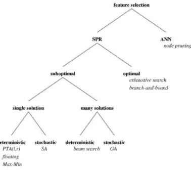
Figure 2.5 and 2.6 show common feature selection models and feature selection algorithms, respectively.

We develop our own feature selection approach based on how useful a feature is in separat-ing a rectangular region from the rest of the image.

Figure 2.5: Feature selection models5

(26)

Figure 2.6: Feature selection algorithms6

(27)

Chapter 3 Overview of Energy Minimization

Framework

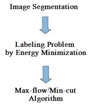
The proposed algorithm implements automatic segmentation using the tool of graph cuts, which works in the energy optimization framework. The task of binary image segmentation is posed as a binary labeling problem, and solved by minimization a energy function. The resulting energy function can be globally and optimally solved with the max-flow/min-cut al-gorithm. Figure 3.1 below shows the way to solve image segmentation problem in the energy optimization framework.

Figure 3.1: Solving image segmentation problem in energy minimization framework

In the optimization framework, there are two major steps, the formulation of energy function and the optimization of it. There are many advantages to the optimization based approach, though it is difficult to formulate appropriate energy function, and to optimize them are not trivial tasks, either. First, it provides a common framework which abstracts useful constraints from details of each particular problem. Once an energy function is formulated, the standard optimization approaches can be applied to solve it. Secondly, it enables us to apply our prior knowledge to solve the problem by encoding it in the energy function. Thus we can expect the

(28)

16 Chapter3. Overview ofEnergyMinimizationFramework

desired solution to have some nice global properties, such as the overall smoothness. Finally, the value of the energy function provides an effective way to evaluate the solution and can be used as a guide in the optimization algorithm [52].

Graph cuts is an optimization algorithm in energy minimization framework, which has been successfully used for a wide variety of vision problems, including image restoration [11, 12, 28, 34], stereo and motion [6, 11, 12, 33, 38, 41, 65, 50, 64], image synthesis [45], image segmentation [9], voxel occupancy [42], multicamera scene reconstruction [69], and medical imaging [7, 8, 39, 37]. The output of graph cuts algorithms is generally a solution with some interesting theoretical quality guarantee. In some cases, the solutions are the global minimum, even though in some case [11, 28, 33, 34, 50], it is a local minimum, but still within a known factor of the global minimum [12]. The experimental results produced by graph cuts algorithm are also quite good [43].

In this chapter, we will go over the energy optimization framework and introduce graph cuts algorithm.

3.1 From Segmentation to Labeling Problem

The goal of segmentation is to simplify and/or change the representation of an image into something that is more meaningful and easier to analyze [67]. Image segmentation is typically used to locate objects and boundaries (lines, curves, etc.) in images. In computer vision, seg-mentation is the process of partitioning an image into multiple segments (sets of pixels, also known as superpixels). More precisely, image segmentation is the process of assigning a label to every pixel in an image such that pixels with the same label share certain visual characteris-tics.

A labeling problem is, roughly speaking, the task of assigning an explanatory “label” to each element in a set of observations [17]. Many classical clustering problems are also labeling problems because each data point is assigned a cluster label. Obviously, we can pose the task of image segmentation as a labeling problem, too.

To describe a labeling problem, one needs a set of observations (the data) and a set of pos-sible explanations (the labels). A discrete labeling problem associates one discrete variable with each datum, and the goal is to find the best overall assignment to these variables (a “label-ing”) according to some criteria. In computer vision, the observations can be things like pixels in an image, salient points within an image, depth measurements from a range-scanner, or in-tensity measurements from CT/MRI. The labels are typically either semantic (car, pedestrian, street) or related to scene geometry (depth, orientation, shape, texture) [17].

The goal in a labeling problem is to construct a map f : P 7→ L that assigns to each ele-ment p ∈ Pa corresponding label fp. The setP indexes the observations, and the label set

(29)

3.2. EnergyFunctionConstruction 17

In image segmentation, the map f is to assign labels fpto image pixels such that∀p∈ P, fp ∈

L, where fpis the label assigned to pixelp,Lis the set of possible labels, andP={1,2, . . . ,P}

is the set of image pixels. If the label set for all pixels is the same, i.e.L, then the set of possi-ble labelings isL= L×L× · · · ×L. That is, the total number of different labelings is as huge asLp_.

For binary image segmentation, the label setL ={0,1}, where 0 and 1 stand for the background and the foreground, respectively. In this thesis, we will focus on binary labeling problem.

3.2 Energy Function Construction

3.2.1 Objective Function

The first step of optimization problem is to formulate an objective function, which maps any so-lution to a real number. In this way, we get a quantity measurement of how good the soso-lution is.

An objective function f : X 7→ Y with Y ⊆ _R is a function which subjects to optimiza-tion [78]. The codomainYof an objective function as well as its range must be a subset of the real numbers (Y ⊆_R).

Generally speaking, the objective function should be incorporated with the constraints that an acceptable solution must satisfy. A good objective function should assign high goodness score to solutions that match the constraints well. In computer vision, the objective function is usually referred to as energy function.

In particular, when designing an energy function, we should make sure it maps a good so-lution to low energy, and a bad soso-lution will get a high energy. For example, in figure 3.2, the right image is the reshuffled image of the one on the left. Although the histograms of the left and right images are the same, the left image is more spatially coherent in its color distribution, so the energy of the solution on the left should be much lower than the energy of the solution on the right.

(30)

There are two commonly used constraints in designing an energy function in image segmen-tation, the data constraint and the smoothness constraint. The data constrain comes from the observed data. It requires the solution to be close to the observed data.

Figure 3.3: Swan

For example, in swan image (figure 3.3), it is easy to come up with the constraint that the pixels that belong to the swan should have lighter colors, and the background pixels should have darker colors. Otherwise, they are violating the data constraints provided by the color information of the image [52].

The smoothness constraint usually encodes our preference for spatial coherence of the labels. Intuitively, most physical world objects are coherent in space. If a pixel in an image belongs to an object, the nearby pixels are very likely to belong to the same object. In other words, the smoothness knowledge tells us that both the background and the object should be spatially coherent. At the same time, we can encode more prior constraints in the energy functions, such as a preference for a particular shape [74].

3.3 Optimization Approaches

The second step of the energy minimization framework is to minimize the energy. In general, this is a very hard problem. The computational task of minimizing the energy is usually quite difficult as it usually requires minimizing a nonconvex function in a space with thousands of dimensions. If the functions have a very restricted form, they can be solved efficiently using dynamic programming [3]. However, researchers typically have needed to rely on general pur-pose optimization techniques such as simulated annealing [4], but it is very slow in practice [43].

(31)

Kol-3.3. OptimizationApproaches 19

mogorov and Zabih [43] describe the conditions on binary energy functions that can be opti-mized exactly with graph cuts, and the energy function satisfing the conditions can be solve in polynomial time.

In our case, we can optimize an energy function exactly and efficiently, using the results from [8] and [43].

3.3.1 Max-flow

/

Min-cut Algorithm

Max-flow/min-cut algorithm can be used to optimize the energy function when dealing with binary labeling problems. Here, we will give a brief summary of related definitions and how to find max-flow/min-cut of a graph.

Figure 3.4: An example of flow1_{from “Introduction to Min-Cut}/_{Max-Flow Algorithms”}

LetG = (V,E) be a network with s,t ∈ Vbeing the source and the sink of G, respectively, where V denotes vertices set and E is edges set. The capacity of an edge is a mapping

c : E 7→ _R+, denoted by c(u,v). It represents the maximum amount of flow that can pass through an edge.

A flow is a mapping f : E 7→ _R+, denoted by f (u,v), subjects to the following two con-straints:

1. fuv ≤ cuv , for each (u,v) (capacity constraint: the flow of an edge cannot exceed its

capacity)

2. P

(u,v)∈E

fu,v = P

(u,v)∈E

fv,u, for each v ∈ V{s,t}(conservation of flows: the sum of the flows

entering a node must equal the sum of the flows exiting a node, except for the source and the sink nodes)

The value of flow is defined by |f| = P

v∈V

fsv, where s is the source of G. It represents the

amount of flow passing from the source to the sink.

1_{Cited from Hong Chen (UCLA CIVS)’s ppt with a bit modification,}_{http://perso.telecom-paristech.}

(32)

Figure 3.5: Left: a s-t cut, right: not a s-t cut

An s− t cut C = (S,T) is a partition ofV such that s ∈ S andt ∈ T. The cut-set of Cis the set{(u,v)∈ E |u∈ S,v∈ T }. Note that if the edges in the cut-set ofCare removed,|f|= 0.

The capacity of ans−tcut is defined byc(S,T)= P

(u,v)∈S×T

cuv. For anys−tcut and flow, the

capacity of s−tcut is the upper-bound of the flow across thes−tcut.

The maximum flow problem is to maximize |f|, that is, to route as much flow as possible fromstot.

The minimum s− t cut problem is minimizing c(S,T), that is, to determineS and T such that the capacity of the s−tcut is minimal.

In optimization theory, max-flow/min-cut theorem is stated as follows:

Theorem [16]: If f is a flow function of as−tgraph, then the follows statements are equiva-lent2_:

A. f is a maximum flow

B. there is as−tcut that its capacity equals to the value of f

C. The residual graph contains no directed path from source to sink.

Max-flow/min-cut theorem means that in a flow network, the maximum amount of flow pass-ing from the source to the sink is equal to the minimum edges’ capacity in all possible way of removing edges. Removing these edges from the network should guarantee no flow can pass from the source to the sink.

There are two main approaches to solve max-flow/min-cut problem for the two-terminal graphs. In Cormen et al. [16], an augmenting path strategy is described to compute the minimum cut of a graph. Goldberg and Tarjan [26] propose an alternative approach named push-relabel to solve the minimum cut problem. Theoretically, the computational cost of minimum cut algorithms is a low order polynomial [52].

(33)

3.4. BinaryImageSegmentation withGraphCuts 21

In [12], Boykov et al. developed new min-cut algorithms, two types of large moves (α −

expansionandα−βswap), which can be used to solve multi-label problem. These algorithms find good approximate solutions by iteratively decreasing the energy on appropriate graphs. Experiment results show that the final solutions do not change significantly by varying the initial labelings. In practice, their algorithm is significantly faster than other standard move algorithms. As a special case of multi-label problem, in this work, we use the α− β swap

algorithm bases on their implementation. For binary submodular energies [8, 43], the swap algorithm finds the exact optimum of the energy function.

3.4 Binary Image Segmentation with Graph Cuts

In this thesis, we deal with the problem of segmenting the foreground object from the back-ground. It can be posed as a binary segmentation problem and can be addressed in the energy optimization framework. This was first done in the work of [8].

The main advantage of segmentation using graph cuts is that it incorporates the appearance of the foreground/background regions into data terms of energy function, meanwhile, constraints on the boundary is incorporated in smoothness term, and the energy function can be easily globally optimized. Here, we briefly review the graph cuts segmentation algorithm of [8].

First, we describe the basic terminology that pertains to graph cuts in binary image segmenta-tion method.

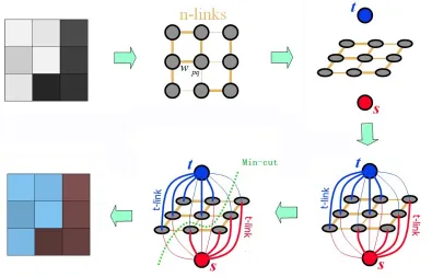
A weighted graph (figure 3.6) G = (V,E) is made up of vertices V and edges E. There are two additional nodes: an object terminal (a source S) and a background terminal (a sink

T). Therefore,V= P ∪ {S,T }. The set of edgesEconsists of two types of undirected edges:

n-links(neighborhood links) andt-links(terminal links). Each pixel phas twot-links{p,S}and

{p,T }connecting it to each terminal. Each pair of neighboring pixels{p,q}inN is connected by an n-link. Without introducing any ambiguity, an n-link connecting a pair of neighbors p

andqwill be denoted by {p,q}. Therefore, E = N S

p∈P

{{p,S},{p,T }}. Each edgee ∈ Ehas a

non-negative costwe.

(34)

A cut is a subset of edgesC ⊂ Esuch that the terminals become separated on the induced graph

G(C)= hV,E \ Ci. The cost of the cutCis the sum of cut edge weights: |C|= P

e∈C

we.

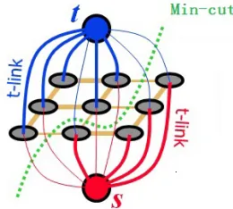
The max-flow/min-cut algorithm [22] can be used to find the minimum cut (the cut with small-est cost) in polynomial time. The segmentation prosess is illustrated as follows (figure 3.7):

Figure 3.7: An example of graph cuts

As mentioned before, image segmentation is posed as a labeling problem, for binary segmen-tation, each pixel in the image has to be assigned a label either foreground or background.

To illustrate binary labeling problem, let P be the set of all pixels in the image, and let N

be the standard 4- or 8-connected neighborhood system onP, pixel pairs{p,q}are neighbour pixels in P. Let fp ∈ L be the label assigned to pixel p. In binary labeling problem, the

la-bel set L = {0,1}, where 0 and 1 stand for the background and the foreground, respectively.

f = nfp | p∈ P

o

denotes the collection of all label assignments.

Energies which can be optimized through graphs cuts usually have the following form:

E(f)= EData(f)+ES mooth(f) (3.1)

where,

EData(f) =

X

p∈P

Dp

fp

(3.2)

ES mooth(f) =

X

{p,q}∈N

Vpq

fp, fq

(35)

3.4. BinaryImageSegmentation withGraphCuts 23

In Eq.(3.1), the first term is called the data term (definded in Eq.(3.2)) which incorporates regional constraints. Specifically, it measures how well pixels fit into the foreground or back-ground models. Dp

fp

is the penalty for assigning label fpto pixelp. The more likelyDp

fp

is for p, the smaller isDp

fp

.

ES mooth(f) is called the smoothness term (definded in Eq.(3.3)), measures the extent to which

f is not smooth. Vpq

fp, fq

is the penalty for assigning labels fp and fqto neighboring pixels.

Most nearby pixels are expected to have the same label, therefore there is no penalty if neigh-boring pixels have the same label, and a penalty otherwise.

Kolmogorov and Zabih [43] prove that if binary energy function is regular3_{, it can be}

opti-mized exactly with a graph cut.

The energy defined in Eq. 3.1 has|P|variables, and it can be viewed as a sum of several two-variableVpq

fp, fq

and single-variableDp

fp

functions. If all of these functions are regular, thenE(f) is regular, see [43]. To check the regularity of the energy functions, we only have to examine the interaction penaltyVpq

fp, fq

. According to [43], all the one variable functions

are regular. Therefore, ifVpq

fp, fq

satisfiesVpq(0,0)+Vpq(1,1)≤Vpq(1,0)+Vpq(0,1), then

E(f) is regular, and it can be optimized by graph cuts.

In our work, the energy function is formulated according to the basic form. The details are described in chapter 6.

3_{A function of two variables} _E₍_x

(36)

Chapter 4 Related Work

Image segmentation is a fundamental problem in computer vision, and it has experienced tremendous growth in the past 10 years. From the extent of user dependence, segmentation algorithms can be categorized into automatic methods and interactive methods. In practice, automatic and interactive methods are often used together to improve the segmentation results. For example, some automatic segmentation methods may require interaction for setting initial parameters and some interactive methods may start with the results from automatic segmenta-tion as an initial segmentasegmenta-tion.

In this chapter, we will give a general summary of the related methods and a brief analysis on them. In particular, since our proposed method target to find an effect automatic initializa-tion for binary image segmentainitializa-tion using graph cuts, we will also talk about some useful cues for starting graph cuts automatically.

4.1 Interactive Segmentation Methods

Interactive image segmentation becomes more and more popular in recent years. Because interactive segmentation gives the user the means to incorporate his knowledge into the seg-mentation process, it often makes the segseg-mentation result more satisfying or to reduce the computing time.

For “interaction”, the user is usually required to click a few “seeds” on the desired object, or near its border, and let the algorithm complete the rest segmentation task. At the same time, the user can edit the results by adding, removing or moving control points (seeds), and re-execute the segmentation algorithm to update the results.

Some popular interactive methods are introduced in this section.

4.1.1 Interactive Graph Cuts

The method of interactive graph cuts for binary image segmentation was first proposed by Boykov and Jolly [8], which is the most important inspiration of this work.

(37)

4.1. InteractiveSegmentationMethods 25

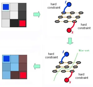
In [8], the user imposes certain hard constraints for segmentation in the way of setting cer-tain pixels (seeds) that absolutely have to be part of the object, and cercer-tain pixels that have to be part of the background. Intuitively, these hard constraints provide clues on what the user intends to segment.

Obviously, the hard constraints by themselves are not enough to obtain a good segmentation. The general energy function mentioned in chapter 3 can be viewed as a soft constraint that incorporates both region and boundary properties for segmentation. In the work of [8], they combine the hard constraints with the soft constraints.

Consider an arbitrary set of data elements P and some neighborhood system represented by a set N of all unordered pairs {p,q}, which are neighboring elements in P. In particular,

P can contain pixels (or voxels) in a 2D (or 3D) grid, and N can contain all unordered pairs of neighboring pixels (voxels) under a standard 8- (or 26-) neighborhood system. Let

f = (f1, . . . , fp, . . . , f|P|) be a binary vector whose components fp that specify assignments to

pixels p in P. Each fp can be either “obj” or “bkg” (abbreviations of “object” and

“back-ground”). In other words, vector f defines a segmentation. Then, the soft constraints that imposed on boundary and region properties of f are described by the energy functionE(f):

E(f)=λ·EData(f)+ES mooth(f) (4.1)

where,

EData(f)=

X

p∈P

Dp

fp

(4.2)

ES mooth(f)=

X

{p,q}∈N

Wpq·δ

fp, fq

(4.3)

δ

fp, fq

=

(

1 i f fp, fq,

0 otherwise

The coefficient λ ≥ 0 in (4.1) specifies a relative importance of the region properties (data) termEData(f) versus the boundary properties (smoothness) termES mooth(f). The regional term

assumes that the the individual penalties for assigning pixel pto object and background, cor-respondinglyDp(“obj”) andDp(“bkg”).

The boundary term comprises the “boundary” properties of segmentation f. CoefficientWpq ≥

0 should be interpreted as a penalty for a discontinuity between pandq. Normally,Wpqis large

when pixels pandqare similar (e.g. in their intensity) andWpq is close to zero when the two

are very different. The penaltyWpqcan also decrease as a function of distance betweenpandq.

The graph used in [8] has the same structure with the general one introduced in the previous chapter, but incorporated with the user input hard constraint (seeds) on corresponding s-link

andt-link. Table 4.1 gives weights of edges inE.

K = 1+max

p∈P

X

{p,q}∈N

(38)

26 Chapter4. RelatedWork

edge weight (cost) for

{p,q} Wpq {p,q} ∈ N

{p,S}

λ·Dp(“bkg00) p∈ P,p<O ∪ B

K p∈ O

0 p∈ B

{p,T }

λ·Dp(“ob j00) p∈ P,p<O ∪ B

0 p∈ O

K p∈ B

Table 4.1: Weights of edges inE

The segmenting process is illustrated in figure 4.1. In the graph, the hard constraints indicate that some pixels were marked as internal and some as external for the given object of interest. The subsets of marked pixels will be referred to as object and background seeds. The segmen-tation boundary can be anywhere but it has to separate the object seeds from the background seeds. In particular, the seeds can be loosely positioned inside the object and background re-gions. Using max-flow/min-cut algorithm, the target image can be segmented automatically by computing a global optimum among all segmentations satisfying the hard constraints.

Figure 4.1: Segmentation with hard constraints

(39)

segmentation can be very efficiently recomputed when the user adds or removes any hard con-straints (seeds). This allows the user to get any desired segmentation results quickly via very intuitive interactions. The process of interactive segmentation is illustrated in figure 4.2.

Figure 4.2: An example of segmentation using interactive graph cuts

Figure 4.2 shows how graph cuts works interactively. The first row illustrates the original im-ages with user interactions: red (foreground brush), blue (background brush). The second row displays the according segmentation results. The degree of user interaction increases from left to right. From the marked pixels, the appearance models for the foreground and the back-ground regions are constructed and used in theDp

fp

terms. For the smoothness term, in this example, image gradient Potts model is used. The user marked seeds are assigned such that

Dp

fp

make it impossible for them to take a label other than the one indicated by the user. That is if the user marks p as the background pixel, then the cost of assigning it to the fore-ground is infinity, and the cost of assigning it to the backfore-ground is 0. This insures that the final segmentation is consistent with user marked seeds.

4.1.2 Grabcut

Grabcut [62] is another inspiration of our method. Actually, it is an iterative graph cuts method. During the process of iteration, the energy can be reduced step by step, hence, it can be used to refine the binary segmentation.

The energy function defined in grabcut is as follows:

E(f)=X

p∈P

Dp

fp

+ X

{p,q}∈N

Vpq

fp, fq

(4.4) where, Dp fp

=−logPrIp| fp

−logπfp

(4.5)

Vpq

fp, fq

=γ X

{p,q}∈N

δ

fp, fq

exp(−βdis(p,q)) (4.6)

and,

β=2

Ip−Iq

2−1

(40)

Pr(·) is a Gaussian probability distribution, and π(·) stand for mixture weighting coefficients.

Ip and fpare intensity and label of p, respectively. The distance here is Euclidean distance in

color space.h·idenotes expectation over an image sample, andγis a constant.

In grabcut algorithm, the initial user input is a rectangle placed loosely around the foreground object (see figure 4.3). The inside is assumed to be mostly the foreground, while the outside of the rectangle is assumed to be the background, and the labels of these pixels will be fixed during the entire segmentation process. From this rough initialization, initial foreground/background models are constructed and binary graph cuts are applied to get the foreground/background segmentation. From this segmentation, the foreground/background models are updated and binary optimization is performed once again. This process is iterated until convergence, in the expectation maximization (EM) [18] manner.

Figure 4.3: Workflow of grabcut method1

The energy function in the grabcut framework optimizes both over the appearance of the fore-ground/background, as well as the segmentation of the image into the new foreground/background parts. Although this problem is no longer optimizable exactly with graph cuts, in [62] they show that the algorithm is guaranteed to converge at least to a local minimum.

(41)

The aim of this thesis is to make grabcut from semi-automatic segmentation algorithm to a fully-automatic one. To be precise, we will try to find the initial “rectangle” of the grabcut algorithm automatically, instead of requiring the user to provide it. After that, we follow the steps of the grabcut algorithm. That is we will run iterative binary graph cuts segmentation to update the foreground/background models until convergence is achieved.

4.1.3 Other Approaches

Besides interactive graph cuts and grabcut, there are other popular interative segmentation methods, just to list a few, here.

• Lazy Snapping

Lazy snapping [49] is another popular graph based segmentation method, which enables the user to edit the result by border editing to get better results.

Actually, lazy snapping algorithm uses a similar graph construction as in graph cuts. The graph vertices in lazy snapping are at a course scale: superpixels (over-segment from wa-tershed algorithm), and then editing border to fix errors on pixel scale. Figure 4.4 below shows the superpixels (left) and border editing (right) in lazy snapping algorithm.

Figure 4.4: Superpixels (left) and border editing (right) in lazy snapping algorithm2

• Snakes

Contour based interactive segmentation “snakes” was suggested by Kass et al. [36] in 1987. The model treats the desired contour as a time evolving curve, and the seg-mentation process is to iteratively reduce the defined energy until convergence, during which the initialized contours actively deform themselves. Convergence is achieved when reaching a balance between the “external” powers that attracts the contour to its place and the “internal” powers which keeps it smooth. The example of segmenting us-ing snakes is illustrated in figure 4.5.

(42)

Figure 4.5: Deformable contour of snakes algorithm

“Snakes” can only find the local minimum of the energy function, so it requires the initialized contour not too far from the object border.

• Livewire

Figure 4.6: Example of livewire algorithm3

Livewire is a shortest path based method, which can reach the global minimum between two user inputted points. It was developed independently by two groups: Mortensen & Barret [58] and Udupa et. al. [21]. Livewire algorithm expects that the user input points should be exactly on the object boundary, which is a strong requirement, while, the graph based segmentation algorithm can perform well as long as there are certain seeds inside and outside the object.

In figure 4.6, the user-cursor path is shown in white. The corresponding detected bound-ary is shown in orange. The current livewire path in an intermediate point is drawn from “free point” through “boundary point” (green segment) to “start point” (orange segment).

(43)

4.2. AutomaticSegmentationMethods 31

4.2 Automatic Segmentation Methods

Although automatic segmentation is a desirable goal in computer vision, we have to admit that fully automatic segmentation is still an open problem.

4.2.1 Saliency Segmentation

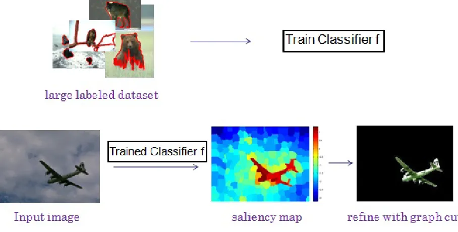
Saliency segmentation [57] is another work related to our approach, we both try to explore an effective initialization to graph cuts, and to a large extent, we are similar in using image features such as color and texture. The main difference between the work in [57] and ours is that the former learns a saliency map that is used to initialize data terms from a manually labeled dataset. In our proposed method, we find foreground region only based on the input image. Other difference is that [57] combines color and texture feature to produce a saliency map. Our approach is to find good features that are useful for distinguishing the foreground from the background.

In [57], the input image is first oversegmented into superpixels. Next, a trained classifier is used to output a confidence value, independently for each superpixel, and the confidence map is also taken to be the saliency map. Then the saliency map is partitioned into classifications of salient object and background. The classifier results will be further refined using iterative graph cuts (see figure 4.7).

Figure 4.7: Saliency segmentation workflow

The energy function in [57] has the basic form defined in [8], and it can be minimized using graph cuts. In particular, the smoothness term is as follow:

Vpq

fp, fq

∝exp−4I2/2σ2·δfp, fq

(44)

where,4I denotes the intensity difference of two neighboring pixels,σ2 is the variance of in-tensity difference of pixels.

The data term consists of two parts,

Dp(1)= −lnPr

Cp|1

−γ·lnmp

(4.9)

Dp(0)= −lnPr

Cp|0

−γ·ln1−mp

(4.10)

where, 1 is the salient object and 0 is the background,Cp is the quantized color of pixel p,mp

is the confidence of pixel p, and constantγcontrols the relative importance of the two parts.

Although saliency segmentation implements automatic segmentation seemingly, it needs large training dataset as pre-condition, which is usually collected and labeled by a human.

4.2.2 Other Automatic Segmentation Methods

There are very few truly automatic segmentation methods that can serve the goal well. They either over-segment the image into small pieces, and then merge by certain techques such as, watershed [75](figure 4.8), meanshift [23](figure 4.9), splitting and merging [30](figure 4.10), normalized cuts [68](figure 4.11), or simply choose a threshold [27](figure 4.12), which is likely to “leak” on the weak boundary.

Figure 4.8: Left: original image, middle: row watershed segmentation, right: watershed segmentation using region marks to control over segmentation4

4_Figure _cited _from

(45)

4.2. AutomaticSegmentationMethods 33

Figure 4.9: Left: original image, right: mean shift result5

Figure 4.10: Left: original image, middle: image after quad spliding, right: image after merging6

Figure 4.11: Left: original image, right: normalized cut result7

Figure 4.12: Left: original image, right: threshoding result8

5_{Figure cited from}_{http://cmp.felk.cvut.cz/cmp/courses/33DZOzima2007/slidy/meanShiftSeg.}

pdf

6_Figure _cited _from _{http://homepages.inf.ed.ac.uk/rbf/CVonline/LOCAL_COPIES/MARBLE/}

medium/segment/split.htm

(46)

4.2.3 Useful Cues for Foreground Initialization

In this thesis, we aim to explore a relatively effective method to start graph cuts, therefore, to make it independent from user guidance. By this indirect way, the goal of automatic segmen-tation might be fulfilled. In this part, we will focus on automatic initialization of graph cuts, and divide them into certain useful cues. Here, we go over some typical methods.

• Machine learning techniques

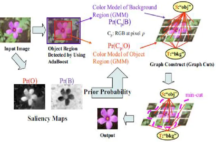
Machine learning techniques are often used to automatically find initial solution for graph cuts. For example, Fukuda et al. [29] use AdaBoost to automatically find the approximate location of the object. A model of saliency-based visual attention is inte-grated with graph cuts since some object regions appear to increase visual attention more than background regions. In this way, the saliency map is used as a prior probability of the object model (spatial information) (see figure 4.13).

Figure 4.13: Graph cuts based on saliency maps and AdaBoost9

We must notice that machine learning approache based on manually labeled dataset for automatic segmentation has a significant drawback, it can only be used to find a specific foreground object/objects that were present in the training dataset. Unfamiliar objects cannot be handled. Obviously, it is not a general method.

Automatic Foreground Initialization for Binary Image Segmentation

Scholarship@Western

Scholarship@Western

Automatic Foreground Initialization for Binary Image

Automatic Foreground Initialization for Binary Image

Segmentation

Segmentation

AUTOMATIC FOREGROUND INITIALIZATION FOR BINARY IMAGE

SEGMENTATION

(Thesis format: Monograph)

by

Wei Li

Graduate Program in Computer Science

A thesis submitted in partial fulfillment

of the requirements for the degree of

Masters of Science

The School of Graduate and Postdoctoral Studies

The University of Western Ontario

London, Ontario, Canada

c

THE UNIVERSITY OF WESTERN ONTARIO

School of Graduate and Postdoctoral Studies

CERTIFICATE OF EXAMINATION

Abstract

Acknowledgements

Contents

List of Figures

List of Tables

List of Appendices

Chapter 1

Introduction

1.1

Overview

1.1.1

Application Prospect of Automatic Image Segmentation

1.1.2

Motivation and Challenge of This Work

1.2

Our Approach

1.2.1

Methodology

1.2.2

The Advantages of Our Method

1.3

Outline of the Thesis

Chapter 2

Image Features

2.1

Feature, Feature Vector and Feature Space

2.2

Feature Types

2.2.1

Texture Descriptors

2.2.2

Color Features

2.3

Feature Selection

Chapter 3

Overview of Energy Minimization

Framework

3.1

From Segmentation to Labeling Problem

3.2

Energy Function Construction

3.2.1

Objective Function

3.3

Optimization Approaches

3.3.1

Max-flow

/

Min-cut Algorithm

3.4

Binary Image Segmentation with Graph Cuts

Chapter 4

Related Work

4.1

Interactive Segmentation Methods

4.1.1

Interactive Graph Cuts