Software Reliability Growth Models Incorporating Burr
Type III Test-Effort and Cost-reliability Analysis
N. Ahmad
1, S. M. K. Quadri
2, M.G.M. Khan
3, and M. Kumar
41
University Department of Statistics and Computer Applications
T. M. Bhagalpur University, Bhagalpur-812007, India
2Department of Computer Science, University of Kashmir, Srinagar, India
3School of Computing, Information and Mathematical Sciences
The University of the South Pacific, Suva, Fiji Islands
4Department of Statistics, Mathematics, and Computer Applications, Rajendra Agriculture University,
Pusa, Samastipur, India
ABSTRACT
Software reliability growth model is one of the fundamental techniques to assess software reliability quantitatively. A number of testing-effort functions for modeling software reliability based on the non-homogeneous Poisson process (NHPP) have been proposed in the past decades. Although these models are quite helpful for the software testing, we still need to put more testing-effort into software reliability modeling. This paper develops a software reliability growth model based on the non-homogeneous Poisson process which incorporates the Burr Type III testing-effort. This scheme has a flexible structure and may cover many of the earlier results on software reliability growth modeling. Models parameters are estimated by the maximum likelihood estimation and the least square estimation methods, and software reliability measures are investigated through numerical experiments on actual data from three software projects. Results are compared with other existing models which reveal that the proposed software reliability growth model has a fairly better prediction capability and it depicts the real-life situation more faithfully. Also, these results can provide a flexible tool on the decision making for software engineers, software scientists, and software managers in the development company. Furthermore, the optimal software release policy for this model based on cost- reliability criteria has been discussed.
Keywords:
Software reliability, testing-effort function, software testing, mean value function, non-homogeneous Poisson process, estimation methods, optimal software release policy.1.
Introduction
A computer system consists of two major components: hardware and software. Although extensive research has been done in the area of hardware reliability, research has also been conducted to study the software reliability of computer systems since 1970. Software reliability is the probability that a given software will be functioning without failure in a given environment during a specified period of time. Hence, software reliability is a key factor in software development process and software quality. The
software development process which includes the following four phases : specification, design, programming and test-and-debug. Many resources are consumed by a software development project. It is assumed that the consumption rate of testing resource expenditures during the testing phase is a constant or even do not consider such testing effort. In reality software reliability models should be developed by incorporating different testing-effort functions. Yamada et al. (1986, 1993, 1990 and 1987) and Musa et al. (1987) proposed a new and simple software reliability growth model which describes the relationship among the calendar testing, the amount of testing-effort, and the number of software errors detected.
Software reliability has been often studied in terms of software reliability growth, based on observed software error data during the software testing phase. Software reliability growth models are concerned with the relation between the cumulative number of errors detected by software testing and the time span of the software testing. Software reliability growth models can estimate the expected initial error content of a software system, the expected number of remaining errors at an arbitrary testing time point, the software reliability, and so on. Several software reliability growth models have been proposed and investigated. For example, Goel & Okumoto (1979), Jelinski & Moranda (1972), Littlewood (1980), Moranda (1979), Musa (1980) and Yamada et al. (1984).
In general appreciable testing resources are spent on software testing in software development. The consumption cure of testing resources over the testing period can be thought of as a testing-effort curve. Testing-effort is measured by: the number of executed test cases, the amount of man-power, and the CPU time spent during the testing phase, and so on. However existing software reliability growth models do not consider such testing-effort; that is, they assume that testing-effort is constant over the testing period. We should consider the effect of testing-effort on software reliability growth in order to develop more realistic software reliability growth models. Parameters are estimated by least square and maximum likelihood estimation method.
difficult to be described by only a Exponential or Rayleigh curve. Although the Weibull-type curve can fit the data well under the general software development environment, it will have an apparent peak phenomenon when the shape parameter m>3. To over come with this difficulty consider Burr type III test –effort function. The Burr type III testing-effort function has the following form:
The cumulative testing-effort consumption in time (0, t] is
W(t)=
1
t
m
0
,
0
4.1
and the current testing effort consumption curve is given as
w(t)=
mt
t
t
m
m
1
1
1 1 10
,
0
,
0
,
0
m
4.2
where , , m and are constant parameters, is the total amount of test-effort expenditure, is the scale parameter, and m and are shape parameters.
The divergence between the Weibull-type curve and W(t) is concentrated in the earlier stages of software development where progress is often least visible and formal accounting procedures for recording the amount of testing effort applied may not have been instituted. It is possible for us to judge between these models using some statistical test of their relative ability to fit actual failure data such as adjusting the origin and scales linearly Parr (1980).
2.1
Least square estimation of parameter
The parameters , ,m
and in the Burr type III testing-effort functions defined by (4.1) or (4.2) can be estimated by least-squares method discussed by Draper & Smith (1981). The estimators for , ,m
and are investigated for testing-effort wk spent at testing time tk (k = 1, 2, ..., n). Then, based on the usual procedures, theleast-squares estimators
ˆ
,
ˆ
,m
ˆ
and
ˆ
be obtained by minimizing the following equation :Minimize,
S
,
,
m
,
n k kk
m
t
W
1 21
log
log
log
Differentiating the above equation with respect to
,
,
m
and
we have the following non-linear equations:
n k kk
m
t
W
s
10
1
1
log
log
log
2
1
0
log
log
log
1 1
n k k n kk
n
m
t
W
n k k n kk m t
W n 1 1 1 log log
log
4.3
n k k k k kk t t
t m t m W s 1 1 0 1 1 1 log log log 2
logWk log mlog1 tk
.
0
1
k k t t
4.4
n k k kk m t t
W m s 1 0 1 log 1 log log log
2
n k k kk m t t
W 1 0 1 log 1 log log
log
4.5
n k k k k k k t t t m t m W s 1 0 1 log 1 log log log 2
0
1 log 1 log log log k k k k k t t t t m W
4.6
These non-linear equations can be solve numerically to
estimate
ˆ
,
ˆ
,
m
ˆ
and
ˆ
.3. Software reliability growth model
A number of SRGMs have been proposed on the subject of software reliability. Among these models, Goel and Okumoto(1979) used an NHPP as the stochastic process to describe the fault process, Lyu (1996), Huang et al. (2002), Berman et al. (1998) and Boehm (2000) modify the G-O model and incorporate the concept of testing-effort in an NHPP model to get a better description of the software fault detection phenomenon. We also propose a new SRGM with the Burr type III testing-effort function to predict the behavior of failure occurrences and the fault content of a software product. Based on our past experimental results, this approach is suitable for estimating the reliability of software application during the development process.
3.1 Model Description
Based on the assumptions given below, if the number of detected errors due to the current testing-effort expenditures is proportional to the number of remaining errors using the Burr type III test effort function in (4.1), we have the following differential equation :
, 0, 0 1 r a t m a r t w t t
m
4.7
where, a is the initial error content in the system & r is the error detection. The solution of differential equation (4.7) gives.
rW t
e
a
t
m
1
4.8
mt r
e
a
t
m
1
1 4.9
From equation (4.8), we have the following important relationship between m(t) & W(t)
t
m
a
a
r
t
W
1
log
4.10
For stochastic modeling of a software-error detection phenomenon, defining the mean value of N(t) based on an NHPP by m(t) in (4.8) yields a software-reliability growth model incorporating the Burr type III test-effort function under the assumptions of Goel and Okumoto (1979) and Yamada (1991) by an NHPP as :
! Pr
n e t m n t N
t m n
n
0
,
1
,
2
,
=
Poim
n
;
m
t
4.11
where m(t) is called mean value function of the NHPP Yamada et al. (1985, 1993) and Poim (n; m (t)) is a Poisson pmf with parameter m(t). The intensity function of the NHPP is given by :
rW te
t
w
r
t
t
m
t
4.12
which means the instantaneous error detection rate. From equation (4.11), we can show that the limit distribution of N(t) is a Poisson distribution with the following mean :
r
e
a
m
1
4.13
The equation (4.13) implies that even if a software system is tested during an infinitely long duration, all errors remaining in the system can not be detection Yamada et al. (1986, 1993). Thus the mean number of undetected errors d(t) is a test is applied for an infinite amount of time is :
r
r
ae
t
d
e
a
a
m
a
1
Assumptions
1.
The error removal process follows the Non Homogeneous Poisson Process (NHPP).2.
The software system is subject to failures at random times caused by errors remaining in the system.3.
The mean number of errors detected in the time interval (t,t
t
]
by the current test-effort is proportional to the mean number of remaining errors in the system.4.
The proportionality is a constant over time. 5. The consumption curve of testing-effort function is described by Burr Type III.6. Each time a failure occurs, the error which caused it is immediately removed, and no new errors are introduced.
3.2 Software reliability measures
Let N(t) represent the number of errors remaining in the system of testing time t. Based on the NHPP model with m(t), given by in equation (4.8), two quantitative measures for software reliability assessment can be derived Goel & Okumoto (1979) and Yamada (1991). The expectation of
t
N
and its variance are given by :
t
E
N
t
E
N
N
t
r
N
E
N
t
E
rW t rWe
e
a
t
m
m
Var
N
t
,
4.14
The software reliability representing the probability that a software failure does not occur in the time interval (t, t + x) is given by :
mtxmte
t
x
R
R
e
a
erW t erWtx
4.15
The instantaneous mean time between failures (MTBF) at arbitrary testing can be defined as a reciprocal of error detection rate in equation (4.12) Yamada (1985). Then the instantaneous MTBF is given by :
rW tt
w
r
t
t
MTBF
.
.
1
1
m t
m
t
t
m
r
t
m
1
.
.
.
.
.
.
.
1
1
1
. 1 1
4.16
4. Maximum likelihood estimations
The reliability growth parameters a and r in the NHPP model with m(t) in (4.7) can be estimated by the method of maximum-likelihood estimation. Let the
estimated parameters
ˆ
,
ˆ
,
m
ˆ
and
ˆ
in the Burr type III test-effort function in (4.1) have been obtained by the method of least-squares estimation. The
ˆ
andr
ˆ
aredetermined for the n observed data pairs
t
k,
y
k
k
1
,
2
,
,
n
.
Then, the joint pmf, the log-likelihood function, for the unknown parameters a and r in the NHPP model with m(t) in (4.7), is given by :
k k
k
k
n
k k
k n
k
t rW t
rW y
y a y y
L
ln lnexp expln 1 1
1 1
1
n
k
k k
n y y
t rW a
1
1!,
ln exp
1
4.17
The usual calculus methods for an interior maximum result in
,
n n
a
f
y
4.18
1
,
1 1 1
k k k k k k n k nf
f
g
g
y
y
g
a
4.19
exp
,
1,2, ,
. , exp n k t W r t W g t W r l f k k k k k
4.20
which can be solved numerically to estimate
a
ˆ
andr
ˆ
.If the sample size n of the observed data is sufficient large, the maximum-likelihood estimates
ˆ
andr
ˆ
asymptotically follow a bivariate s-normal distribution.
,
~
ˆ
ˆ
n
r
a
BVN
r
a
4.21
The in the asymptotic properties of (4.21) is useful in quantifying the variability of the estimated parameters
a
ˆ
andr
ˆ
Nelson (1982), and is the inverse of F
2 2 2 2 2 2ln
ln
ln
ln
r
L
E
r
a
L
E
r
a
L
E
a
L
E
F
=
,
1 1 2 1
k k n k k k n n nf
f
g
g
a
g
g
a
f
4.22
where,
rW tkk
W
t
e
g
4.23
and
tk
rW k
e
f
1
Substitutory the value of a and r in (4.23) and calculate F-1. The estimated asymptotic variance-covariance matrix is :
r
Var
r
a
Cov
r
a
Cov
a
Var
F
ˆ
ˆ
,
ˆ
ˆ
,
ˆ
ˆ
ˆ
15. Real Software Comparison Criteria and
Data Analysis
5.1 Comparison criterion
To check the performance of our software reliability growth model and to make their comparison with the other existing SRGM, we use two types of comparison criteria :
(1)
The Accuracy of Estimation Musa et al. (1987), Hou et al. (1994), Goel et al. (1979) and Kuo et al. (2001).
a aM
m
M
4.24
where Ma is the actual cumulative number of detected errors during the test and after the test, and m is the estimated parameter :
(2)
The Mean of Square fitting Errors
k
m
t
m
MSE
k i k k
1 24.25
The lower MSE indicates less fitting errors and better performance Kapur & Garg (1996).
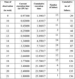
5.2 Actual Data Analysis
The set of real data in Table 4.1 is given. In this chapter is the System T1 data of the Rome Air Development Center (RADC) projects and cited from Musa et al. (1987). The number of object instructions for the system T1 which is used for a real-time command and control application. In this case, the size of the software is approximately 21,700 object instructions. The software were tested for 21 weeks with 9 programmers. During the test phase, about 25.3 CPU Hours were used and 136 faults were detected. In order to estimate the parameters
,
, m
and
of the Burr Type III distributed function; we fit the actual testing-effort data into equations (4.1) and (4.2) and solve it by using the method of least squares. That is, we will minimize the sum of squares given in equation (4.3). Hence, we can find the estimates only through numerical procedures. The estimated values ofparameters of the Burr Type III testing-effort function are:
ˆ =27.54330
ˆ = 0.0528876,
4.26
m
ˆ =0.405062, and
ˆ
= 13.56046
The estimated Burr Type III test-effort functions are
13.560460.405061
13.56046
0.405062052887 . 0 1 54330 . 27 ) (
ˆ
t
W
4.28
Figure 4.1 and Figure 4.2 shows the fitting of the estimated testing-effort by using Equation (4.27) and (4.28). Here, the fitted curves are shown as a doted line and solid line is actual software data. Using the estimated parameters
,
,
m,
and
,
the other parametersa
,
r
in (4.8) can be solved by MLE method.For these estimates, the optimality was checked numerically.
These estimated parameters are
153455
.
0
14062
.
134
r
a
Table 4.2 summarizes the experimental results of estimated parameters with their standard errors and 95 % confidence bound. The estimated mean value function is
0.1534527.543310.0528813.560460.4050621
14061
.
134
)
(
ˆ
te
t
m
4.29
Where
13.5604
0.405062052887
.
0
1
54330
.
27
)
(
ˆ
t
W
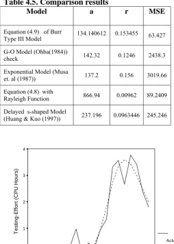
Table 4.3 and 4.4 shows regression analysis depends on test – effort and number of failure respectively. Similarly, we plotted a fitted curve of the estimated mean value function with the actual software data in Figure 4.3. Intensity function also given in Figure 4.4 fitted well in this experiment. Also a comparison Table of the estimates of our model along with other models with initial faults
a
and MSE is given in Table 4.5. From Figures (4.1), (4.2), (4.3) and (4.4) and the comparison criteria in Table 4.5 shows that our SRGM is better fit than the other models for debugging data. Kolmogorov Smirnov goodness-of-fit test shows that our proposed SRGM described by an NHPPwith
m
ˆ
(
t
)
in (4.29) fits pretty well at the 5 % level of significance.).Table 4.1. Software Failure Data ( System T1).
Time of observation
(in week)
Current execution time
(in CPU hr)
Cumulative execution
time
Number of failure
Cumulative no. of failure.
1 0.00917 0.00917 2 2
2 0.01000 0.01917 0 2
3 0.00300 0.02217 0 2
4 0.02300 0.04517 1 3
5 0.04100 0.08617 1 4
6 0.00400 0.09017 2 6
7 0.02500 0.11517 1 7
Time of observation
(in week)
Current execution time
(in CPU hr)
Cumulative execution
time
Number of failure
Cumulative no. of failure.
9 0.97300 1.39017 13 29
10 0.02000 1.41017 2 31
11 0.45000 1.86017 11 42
12 0.25000 2.11017 2 44
13 0.94000 3.05017 11 55
14 1.34000 4.39017 14 69
15 3.32000 7.71017 18 87
16 3.56000 11.27017 12 99
17 2.66000 13.93017 12 111
18 3.77000 17.70017 15 126
19 3.40000 21.10017 6 132
20 2.40000 23.50017 3 135
21 1.80000 25.30017 1 136
Table 4.2 Experimental Result of different
parameters
Parameters Estimate Standard Error
95 % confidence Interval
Lower Upper
Α 27.54330 1.670201 24.01948 31.067121
β 0.05288 .000088 0.0510222 0.054753
m
0.0405062 3.75230 5.642788 21.47713
13.56046 0.138939 0.01119295 0.698199a 134.140612 5.46235 122.70776 145.57346
r 0.153455 0.01866 0.144393 .19251
Table 4.3 Regression analysis depends on
test-effort
Source Degree of Freedom
Sum of squares
Mean Squares
Regression 4 2369.05331 592.26333
Residual 17 2.94673 0.17334
Un corrected
Total 21 2372.0004 - (Corrected
Total) 20 1447.35951 -
Table 4.4 Regression Analysis depends on
Number of failures
Source
Degree of Freedom
Sum of squares
Mean Squares
Regression 2 112046.03571 56023.0178
Residual 19 1331.96429 70.10338
Un corrected
Total 21 213378.000 - (Corrected
Total) 20 51709.23810 -
R
2= 1-Residual SS/Corrected SS = 0.97424
Table 4.5. Comparison results
Model a r MSE
Equation (4.9) of Burr
Type III Model 134.140612 0.153455 63.427 G-O Model (Ohba(1984))
check 142.32 0.1246 2438.3
Exponential Model (Musa
et. al (1987)) 137.2 0.156 3019.66
Equation (4.8) with
Rayleigh Function 866.94 0.00962 89.2409 Delayed s-shaped Model
(Huang & Kuo (1997)) 237.196 0.0963446 245.246
Figure 4.1. Observed/estimated Current Testing-Effort Function VS. Time Time (Weeks)
21 19 17 15 13 11 9 7 5 3 1
T
e
s
ti
ng-E
ffor
t (
C
P
U
H
our
s
)
4
3
2
1
0
Actual
Estimated
Figure 4.2. Observed/estimated Cumulative Test-Effort Function VS. Time Time (Weeks)
21 19 17 15 13 11 9 7 5 3 1
C
u
m
u
la
ti
ve T
e
sti
n
g-E
ffor
t (
C
P
U
H
o
ur
s)
30
20
10
0
Observed
Estimated
Figure 4.3. Observed/Estimated Cumulative Number of Failures VS. Time
Time (Weeks)
21 19 17 15 13 11 9 7 5 3 1
C
um
ul
at
iv
e N
um
ber
of
F
ai
lur
es
160
140
120
100
80
60
40
20
0
Observed
Estimated
0 2 4 6 8 10 12 14 16 18 20
1 3 5 7 9 11 13 15 17 19 21
Time (weeks)
In
te
ns
it
y
F
u
nc
ti
o
n
4.7. Conclusion
In this chapter, test effort function representing the time dependent behavior of test effort spent during software testing phase have been described by Burr Type-III curve. Due to incorporating the Burr Type – III testing effort function the proposed software reliability growth model fits the real software data set fairly well and in could give us reasonable description of resource consumption behavior. Comparison study shows that Burr Type – III model gives minimum error percentage rather than, G-O, Exponential Rayleigh and Delayed S-shaped model. From figure we also conclude that our model fit the better as compare to other models.
References
[1] Ahmad, N., Bokhari, M.U., Quadri, S.M.K. and Khan, M.G.M. (2008), “The exponetiated Weibull software reliability growth model with various testing-efforts and optimal release policy: a performance analysis”, International Journal of Quality and Reliability Management, Vol. 25 (2), pp. 211-235.
[2] Ahmad, N., Quadri, S. M. K. and Choudhary, N. (2006), “Design of Accelerated life Tests for Periodic Inspection with Burr Type III Distributions: Models, Assumptions, and Applications,” Journal of Applied Statistical Science, Vol. 15 (2), 161 – 179.
[3] Ahmad, N., Quadri, S. M. K. and Choudhary, N. (2008), “Design of Accelerated life Tests for Periodic Inspection with Burr Type III Distributions: Models, Assumptions, and Applications,” Trends in Applied Statistics Research (ISBN 978-1-60456-153-1), Editor: M. Ahsanullah, Nova Science Publishers, Inc, USA, pp. 27– 46.
[4] Al-Dayian G. R. (1999), “Burr type III distribution: Properties and Estimation”, The Egyptian Statistical Journal, 43, pp. 102-116.
[5] Bokhari, M.U. and Ahmad, N. (2006), “Analysis of a software reliability growth models: the case of log-logistic test-effort function”, In: Proceedings of the 17th IASTED International Conference on Modelling and Simulation (MS’2006), Montreal, Canada, pp. 540-545.
[6] Bokhari, M.U. and Ahmad, N. (2007), “Software reliability growth modeling for exponentiated Weibull functions with actual software failures data”, Advances in Computer Science and Engineering: Reports and Monographs, Vol. 2, World Scientific Publishing Company.
[7] Burr, I.W. (1942), “Cumulative frequency distribution”, Annals of Mathematical Statistics, Vol. 13, pp. 215-231.
[8] Domma, F. (2010), “Some properties of the bivariate Burr type III distribution”, Statistics: A Journal of Theoretical and Applied Statistics, Vol. 44, no. 2, pp. 203-215.
[9] Goel, A.L. and Okumoto, K. (1979), “Time dependent error-detection rate model for software reliability and other performance measures”, IEEE Transactions on Reliability, Vol. R- 28, No. 3, pp. 206-211.
[10] Huang, C.Y. (2005), “Performance analysis of software reliability growth models with testing-effort and change-point”, Journal of Systems and Software, Vol. 76, pp. 181-194.
[11] Huang, C.Y. and Kuo, S.Y. (2002), “ Analysis of incorporating logistic testing-effort function into software reliability modeling”, IEEE Transactions on Reliability, Vol. 51, no. 3, pp. 261-270.
[12] Huang, C.Y., Kuo, S.Y. and Chen, I.Y. (1997), “Analysis of software reliability growth model with logistic testing-effort function”, In: Proceeding of 8th International Symposium on Software Reliability Engineering (ISSRE’1997), Albuquerque, New Maxico, pp. 378-388.
[13] Huang, C.Y., Kuo, S.Y. and Lyu, M.R. (1999), “Optimal software release policy based on cost, reliability and testing efficiency”, In: Proceedings of the 23rd IEEE Annual International Computer Software and Applications Conference (COMPSAC’99), Phoenix, Arizona, pp. 468-473.
[14] Huang, C.Y., Kuo, S.Y. and Lyu, M.R. (2000), “Effort-index based software reliability growth models and performance assessment”, In: Proceedings of the 24th IEEE Annual International Computer Software and Applications Conference (COMPSAC’2000), pp. 454-459.
[15] Huang, C.Y., Kuo, S.Y. and Lyu, M.R. (2007), “An assessment of testing-effort dependent software reliability growth models”, IEEE Transactions on Reliability, Vol. 56, no.2, pp 198-211.
[16] Kapur, P.K. and Garg, R.B. (1989), “Cost reliability optimum release policies for a software system under penalty cost”, International Journal of System Science, Vol. 20, pp. 2547-2562.
[17] Kapur, P.K. and Garg, R.B. (1990), “Cost reliability optimum release policies for a software system with testing effort”, Operations Research, Vol. 27, no. 2, pp. 109-116.
[18] Kapur, P.K. and Younes, R.B. (1996) “Modeling an imperfect debugging phenomenon in software reliability”, Microelectronics and Reliability, Vol. 36, pp. 645-650.
[19] Kapur, P.K., Garg, R.B. and Kumar, S. (1999), Contributions to Hardware and Software Reliability, World Scientific, Singapore.
[20] Kapur, P.K., Goswami, D.N. and Gupta, A. (2004) “A software reliability growth model with testing effort dependent learning function for distributed systems”, International Journal of Reliability, Quality and Safety Engineering, Vol. 11, no. 4, pp. 365-377.
[21] Kapur, P.K., Grover, P.S., and Younes, S. (1994), “Modeling an imperfect debugging phenomenon with testing effort”, In: Proceedings of 5th International Symposium on Software Reliability Engineering (ISSRE’1994), pp. 178-183. [22] Kumar, M., Ahmad, N. and Quadri, S.M.K. (2005), “Software reliability growth models and data analysis with a Pareto test-effort”, RAU Journal of Research, Vol., 15 (1-2), pp. 124-128.
[23] Kuo, S.Y., Hung, C.Y. and Lyu, M.R. (2001), “Framework for modeling software reliability, using various testing-efforts and fault detection rates”, IEEE Transactions on Reliability, Vol. 50, no.3, pp 310-320.
[24] Lyu, M.R. (1996), Handbook of Software Reliability Engineering, McGraw- Hill.
[25] Mokhlish, N. A. (2005) “Reliability of a Stress-Strength Model with Burr Type III Distributions, ”Communications in Statistics: Theory and Methods, 34(7), 1643–1657.
[26] Musa J.D. (1999), Software Reliability Engineering: More Reliable Software, Faster Development and Testing, McGraw-Hill.
[27] Musa, J.D., Iannino, A. and Okumoto, K. (1987), Software Reliability: Measurement, Prediction and Application, McGraw-Hill.
[28] Nelson, W. (1982), Applied Life Data Analysis, Wiley, New York.
[29] Ohba, M. (1984), “Software reliability analysis model” IBM Journal. Research Development, Vol. 28, no. 4, pp. 428-443. [30] Okumoto, K. and Goel, A.L. (1980), “Optimum release time for software system based on reliability and cost criteria,” Journal of Systems and Software, Vol.1, pp. 315-318.
[31] Pham, H. (2000), Software Reliability, Springer-Verlag, New York.
[33] Pillai, K. and Nair, V.S.S. (1997), “A model for software development effort and cost estimation”, IEEE Transactions on Software Engineering, Vol. 4, no. 8, pp. 343-361.
[34] Quadri, S.M.K., Ahmad, N., Peer, M.A. and Kumar, M. (2006), “Nonhomogeneous Poisson process software reliability growth model with generalized exponential testing effort function”, RAU Journal of Research, Vol., 16 (1-2), pp. 159-163. [35] Shao Q., Chen Y. D. and Zhang L. (2008), “An extension of three-parameter Burr III distribution for low-flow frequency analysis”, Computational Statistics & Data Analysis, 52, pp. 1304-1314.
[36] Tohma, Y., Jacoby, R., Murata, Y. and Yamamoto, M. (1989), “Hyper-geometric distribution model to estimate the number of residual software fault”, In: Proceeding of COMPSAC-89, Orlando, pp. 610-617.
[37] Xie, M. (1991), Software Reliability Modeling, World Scientific Publication, Singapore.
[38] Yamada, S., Hishitani J. and Osaki, S. (1991), “Test-effort dependent software reliability measurement”, International Journal of Systems Science, Vol. 22, no. 1, pp. 73-83.
[39] Yamada, S., Hishitani J. and Osaki, S. (1993), “Software reliability growth model with Weibull testing-effort: a model and application”, IEEE Transactions on Reliability, Vol. R-42, pp. 100-105.
[40] Yamada, S., Narihisa, H. and Osaki, S. (1984), “Optimum release policies for a software system with a scheduled software delivery time”, International Journal of System Science, Vol.15, pp. 905-914.
[41] Yamada, S. and Ohtera, H. (1990), “Software reliability growth models for testing effort control”, European Journal of Operational Research, Vol. 46, no. 3, pp. 343-349.
[42] Yamada, S., Ohtera, H. and Norihisa, H. (1986), “Software reliability growth model with testing-effort”, IEEE Transactions on Reliability, Vol. R-35, no. 1, pp.19-23.
[43] Yamada, S., Ohtera, H. and Narihisa, H. (1987), “A testing-effort dependent software reliability model and its application”, Microelectronics and Reliability, Vol. 27, no. 3, pp. 507-522.
[44] Yamada, S., and Osaki, S. (1985a), “Software reliability growth modeling: models and applications”, IEEE Transaction on Software Engineering, Vol. SE-11, no. 12, pp. 1431-1437.