Spatiotemporal Forecasting At Scale

Scholarship@Western

Scholarship@Western

Electronic Thesis and Dissertation Repository

8-13-2019 11:00 AM

Spatiotemporal Forecasting At Scale

Spatiotemporal Forecasting At Scale

Rafael Felipe Nascimento de Aguiar The University of Western Ontario

Supervisor

Capretz, Miriam A. M.

The University of Western Ontario

Graduate Program in Electrical and Computer Engineering

A thesis submitted in partial fulfillment of the requirements for the degree in Master of Engineering Science

© Rafael Felipe Nascimento de Aguiar 2019

Follow this and additional works at: https://ir.lib.uwo.ca/etd

Part of the Software Engineering Commons

Recommended Citation Recommended Citation

Nascimento de Aguiar, Rafael Felipe, "Spatiotemporal Forecasting At Scale" (2019). Electronic Thesis and Dissertation Repository. 6316.

https://ir.lib.uwo.ca/etd/6316

This Dissertation/Thesis is brought to you for free and open access by Scholarship@Western. It has been accepted for inclusion in Electronic Thesis and Dissertation Repository by an authorized administrator of

Spatiotemporal forecasting can be described as predicting the future value of a variable given

when and where it will happen. This type of forecasting task has the potential to aid many

institutions and businesses in asking questions, such as how many people will visit a given

hospital in the next hour. Answers to these questions have the potential to spur significant

so-cioeconomic impact, providing privacy-friendly short-term forecasts about geolocated events,

which in turn can help entities to plan and operate more efficiently.

These seemingly simple questions, however, present complex challenges to forecasting

sys-tems. With more GPS-enabled devices connected every year, from smartphones to wearables

to IoT devices, the volume of collected spatiotemporal data that accompanies these questions

has exploded, following the Big Data trend. This thesis proposes a forecasting framework that

employs distributed computing in order to scale its internal components and overcome this

high data volume scenario. It also designs discretization components that allow for flexibility

in the framing of the forecasting questions. Furthermore, it devises a Geographically Global

Model (GGM) backed by an ensemble of Stochastic Gradient Boosted Trees, a collection of

Geographically Local Models (GLMs) backed by ARIMA models, and a non-linear blending

of those as part of its multistage machine learning pipeline in order to boost its performance

and stability.

The merit of the proposed research is evaluated in three experiments, each of which

com-prises millions of records, namely forecasting hourly taxi demand in the city of New York,

forecasting daily crime density in the city of Chicago, and forecasting hourly visits to places

of interest across Canada. The experimental results show the effectiveness of the proposed

Spatiotemporal Forecasting Frameworkin forecasting stable results across the three domains,

while also outperforming the naive baseline by at least 49.8% with respect to the SMAPE

residuals.

Keywords:Spatiotemporal, Forecasting, Big Data, Distributed Computing, Ensemble

Learn-ing, BlendLearn-ing, Local Learning

Spatiotemporal forecasting can be described as predicting the future value of a variable given

when and where it will happen. This type of forecasting task has the potential to aid many

institutions and businesses in asking questions, such as how many people will visit a given

hospital in the next hour. Answers to these questions have the potential to spur significant

so-cioeconomic impact, providing privacy-friendly short-term forecasts about geolocated events,

which in turn can help entities to plan and operate more efficiently.

These seemingly simple questions, however, present complex challenges to forecasting

sys-tems. With more GPS-enabled devices connected every year, from smartphones to wearables

to IoT devices, the volume of collected spatiotemporal data that accompanies these questions

has exploded, following the Big Data trend. This thesis proposes a forecasting framework that

employs distributed computing in order to scale its internal components and overcome this high

data volume scenario. It also designs discretization components that allow for flexibility in the

framing of the forecasting questions.

The merit of the proposed research is evaluated in three experiments, each of which

com-prises millions of records, namely forecasting hourly taxi demand in the city of New York,

forecasting daily crime density in the city of Chicago, and forecasting hourly visits to places

of interest across Canada. The experimental results show the effectiveness of the proposed

Spatiotemporal Forecasting Frameworkin forecasting stable results across the three domains,

while also outperforming the naive baseline by at least 49.8%.

I thank God for every person you sent my way. The person that I am today is, without a doubt,

much better because of everything that I learned from them and all the moments I shared with

them.

I want to thank my supervisor Dr. Miriam Capretz, for seeing potential in me and opening

the doors to Western University. Also, I would like to say that I sincerely appreciate your

guidance and the effort you put in helping me with this research.

To my colleagues, fellow TAs, students, and faculty members at Western University a big

thanks. My graduate school years were fantastic because of all of you.

To Dr. Abdelkader Ouda, I extend my heartfelt gratitude. I learned a lot while I was a TA

under your supervision.

I would also like to extend my appreciation to the incredibly talented and helpful people

from Western University’s Writing Centre, and Map and Data Centre. Your support was of

exceptional value to me.

To my cousin Lilo, Thamiris and Donatello, I’ll be forever grateful for your support here in

Canada. Thank you for always being there for me.

To my father, mother, brother, sister, family and friends, you are the joy of my life. Thank

you all so much for your kindness and encouragement.

To my wife, I could not have done any of this without you. Thank you for making my life

a whole lot better.

Abstract ii

Summary for Lay Audience iii

Acknowledgements iv

List of Figures viii

List of Tables x

1 Introduction 1

1.1 Motivation . . . 3

1.2 Contributions . . . 5

1.3 Thesis Organization . . . 6

2 Background and Literature Review 8 2.1 Feature Discretization . . . 8

2.1.1 Equal Width Discretization . . . 9

2.1.2 Grid-based Discretization . . . 9

2.2 Time Series Forecasting Models . . . 14

2.3 Machine Learning . . . 15

2.3.1 Tree-based Ensembles . . . 16

2.3.2 Blending Models . . . 21

2.3.3 Local Learning . . . 22

2.4 Distributed Computing And Scalability . . . 23

2.5 Literature Review . . . 24

2.5.1 Linear Models . . . 26

2.5.2 Neural Networks . . . 27

2.5.3 Ensemble Models . . . 29

2.6 Summary . . . 30

3 Spatiotemporal Forecasting Framework 32 3.1 Data Preprocessing . . . 34

3.1.1 Temporal Discretization . . . 34

3.1.2 Spatial Discretization . . . 35

3.1.3 Data Cleaning . . . 37

3.1.4 Large Scale Aggregation . . . 40

3.2 Multistage Machine Learning Pipeline . . . 42

3.2.1 Geographically Global Model . . . 43

3.2.2 Geographically Local Models . . . 44

3.2.3 Blending Model . . . 48

3.3 Summary . . . 54

4 Evaluation 56 4.1 Implementation . . . 56

4.2 Experiments . . . 62

4.2.1 New York City Taxi Trips . . . 64

4.2.2 Crimes in The City of Chicago . . . 70

4.2.3 Visits to Places of Interest Across Canada . . . 76

4.2.4 Discussion . . . 82

4.3 Summary . . . 85

5.1 Conclusions . . . 86

5.2 Future Work . . . 87

Bibliography 90

Curriculum Vitae 98

2.1 Grid-based discretization of the Earth . . . 11

2.2 Illustration of two levels of subdivision of the unit square . . . 11

2.3 Six iterations of the Hilbert Curve . . . 13

2.4 Unfolded Earth cube indexed by a global Hilbert Curve . . . 14

2.5 Decision Tree region boundaries in a 2-dimensional (latitude, longitude) fea-ture space . . . 18

2.6 Decision Tree nodes with their predicates in boldface, leaves with their under-lying records (described in a set), and predictions at the lower bottom . . . 19

2.7 Time-sliding window for cross-validation . . . 23

2.8 Distributed Computing vs. Parallel Computing . . . 25

3.1 Spatiotemporal Forecasting Framework Overview . . . 33

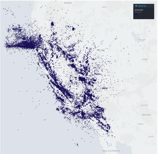
3.2 Earthquakes in the state of California from 1967 to 2018 . . . 38

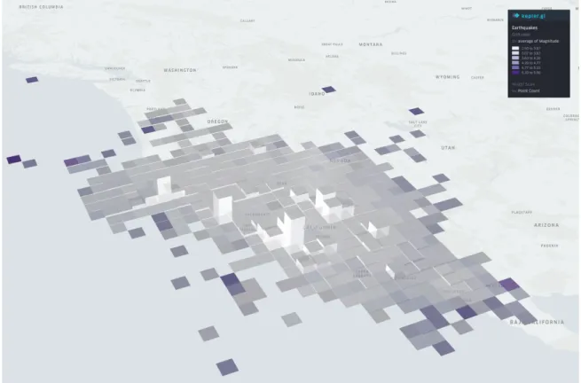
3.3 Earthquakes in the state of California from 1967 to 2018 after discretization and aggregation processes . . . 39

3.4 A geo-located polygon (in red) representing an area of interest . . . 40

3.5 Three spatial grids covering the same geographical region (not to scale) at dif-ferent resolutions . . . 46

3.6 A discretized map of Manhattan . . . 47

3.7 Supporting Class Diagram . . . 49

3.8 Stage 0 - Training Of The Base Models. . . 50

3.9 Stage 1 - Training Of The Blending Model. . . 53

4.1 Docker Containers vs. Virtual Machines . . . 58

4.2 Spark Cluster Architecture Overview . . . 59

4.3 Polygons in grey representing the spatial filter over the Manhattan region. . . . 66

4.4 NYC Taxi Trips – Average SMAPE per hour on a small sample of the testing

data . . . 68

4.5 NYC Taxi Trips – Average RMSE per hour on a small sample of the testing data 69

4.6 NYC Taxi Trips – SMAPE box plot . . . 70

4.7 Polygons in grey representing the spatial filter over the Chicago region. . . 72

4.8 Chicago Crimes – Average SMAPE per day on a small sample of the testing data. 74

4.9 Chicago Crimes – Average RMSE per day on a small sample of the testing data. 75

4.10 Chicago Crimes – SMAPE box plot . . . 76

4.11 Polygons in grey representing the spatial filter across the Canadian landscape. . 78

4.12 Visits to Places of Interest Across Canada – Average SMAPE per hour on a

small sample of the testing data . . . 80

4.13 Visits to Places of Interest Across Canada – Average RMSE per hour on a small

sample of the testing data . . . 81

4.14 Visits to Places of Interest Across Canada – SMAPE box plot . . . 82

4.15 Average SMAPE per model across experiments. . . 84

3.1 Examples of timestamp truncations at arbitrary resolutions. . . 35

3.2 Examples of the discretization of spatial coordinates at arbitrary resolutions. . . 36

3.3 Spatiotemporal records before aggregation . . . 42

3.4 Records after density-based spatiotemporal aggregation. . . 42

3.5 Geographically Global Model Input Features . . . 44

3.6 Sample spatiotemporal data . . . 45

3.7 Data from Table 3.6 after the spatial partitioning step . . . 45

4.1 NYC Taxi Trips – Dataset Statistics . . . 64

4.2 NYC Taxi Trips – Dataset Statistics After Preprocessing. . . 65

4.3 GGM – Stochastic Gradient Boosted Trees Hyperparameters. . . 67

4.4 NYC Taxi Trips – Model Metrics Across All Testing Windows . . . 69

4.5 Chicago Crimes – Dataset Statistics. . . 70

4.6 Chicago Crimes – Dataset Statistics After Preprocessing. . . 71

4.7 Chicago Crimes – Model Metrics Across All Testing Windows . . . 76

4.8 Visits to Places of Interest Across Canada – Dataset Statistics. . . 77

4.9 Visits to Places of Interest Across Canada – Dataset Statistics After Prepro-cessing. . . 78

4.10 Visits to Places of Interest Across Canada – Model Metrics Across All Testing Windows . . . 82

Introduction

Spatiotemporal forecasting has been applied to a diverse number of domains, including crime,

influenza, taxi demand, and visits forecasting. When used for crime forecasts, this technique

can alert police officers to developing crime patterns in a city, helping them to coordinate

patrols in order to better fight crime, for example [20]. In influenza forecasting, this technique

can provide insights into which hospitals will see more demand in the next influenza season,

helping health-care practitioners to prepare accordingly [52]. In the taxi demand prediction,

spatiotemporal forecasting can assist with the placement of drivers so that they can quickly

reach passengers, saving time and reducing overall costs [66]. Spatiotemporal forecasting can

also be utilized to estimate the anticipated number of visits that a site will receive, providing the

manager with foot-traffic information that they could leverage to optimize their staffschedule

and better serve customers [27].

A spatiotemporal dataset is a collection of records with labels showing where and when

they were collected [23]. More formally, it is a dataset sampled from a process that has both

spatial and temporal components. Even more specifically, in this research, a spatiotemporal

dataset is sampled from temporal and geographical spaces. That is, it contains a timestamp

denoting when it happened and a pair of latitude and longitude coordinates that identify where it

happened on Earth. Frequently this “when” label comes from the device’s system clock and the

“where” label comes from a satellite-based radio-navigation system like the Global Positioning

System (GPS) that tracks the positions of receivers on Earth. Because of the ubiquity of GPS, it

is common to refer to latitude and longitude as GPS coordinates, and it is also accepted to refer

to location-aware devices as “GPS-aware” or “GPS-enabled”; this research uses these terms

interchangeably henceforth.

A concrete example of a spatiotemporal dataset could be a dataset that describes the

occur-rence of earthquakes while containing the timestamp of when they happened, the GPS

coordi-nates of where the center of the earthquake was, and potentially some associated measurements

such as the magnitude of the earthquake and the depth from the epicentre to the surface.

The task of predicting out-of-sample values of a variable based on historical data is denoted

as a prediction task in the research field of Machine Learning [31]. For researchers in the field

of Time Series, however, the term “forecasting” carries the same meaning, with the added

connotation of predicting the future values of a random variable [65]. Henceforth, this thesis

utilizes the terms “prediction” and “forecasting” interchangeably to mean the prediction of

future values. What this work sets out to do, then, is to provide a domain agnostic, scalable

framework that can answer a predictive question of the form: given an input feature vector x,

an arbitrary timestampt, and a location s, what is the forecasted value of a target variable ˆy(x)

att+1?

A fundamental facet of that question is the spatial (S) and temporal resolution (T) of the

study. In other words, assuming sufficient resolution in the initial underlying data, one could

ask forecasting questions based on longer time intervals or wider regions of interest. Taking the

previously mentioned earthquake dataset as a basis, and assuming an initial temporal resolution

of seconds and a spatial resolution at the city block level, one could conceivably ask questions

similar to the following:

1. ˆy(x)t+1,s |t ∼T(hourly)∧s∼ S(city block)

3. ˆy(x)t+1,s |t ∼T(monthly)∧s∼ S(1km2area)

The first of these questions models a one-hour-ahead forecast at the city block level, the

second models a one-day-ahead forecast at the city level, and the third models a next-month

forecast for spatial regions that comprise a 1km2area. The appropriate resolution for the spatial

and temporal variables ultimately depends on which forecasting questions a user wants to

an-swer. For example, it might be sensible to forecast a macro event, such as an earthquake, at the

daily resolution and city level because of how its aftermath can wreak chaos in large regions

for an entire day. On the other hand, for other types of events, such as taxi demand, an hourly

forecast at the city block level might be more appropriate as drivers would have predictions that

would be more in line with the transit patterns of a car. Another essential facet is the volume of

historical data. In terms of time frame, volume relates to how many months, years or decades

of data are available, for example. In terms of geographical extension, volume relates to how

many neighbourhoods, cities, or states the data cover.

1.1

Motivation

The gathering of space and time contextualized information about people’s offline behaviour,

has made it possible for businesses and institutions to use forecasting techniques to ask

ques-tions such as: how many visits will this coffee shop experience in the next hour? A significant

challenge in this type of forecasting comes from the fact that the underlying datasets are

in-creasingly growing, following the Big Data trend [52]. With more GPS-enabled devices being

connected every year, from smartphones to wearables to IoT devices, the amount of collected

geolocated data has been exploding [68].

This Big Data volume that increasingly accompanies spatiotemporal datasets poses diffi

cul-ties for the preprocessing algorithms that run in a single pass through the data and even more

so for the training of learning algorithms, which often iterate a few times on the input dataset.

bil-lion records before preprocessing, making it laborious to process it in a reasonable time frame

even in a powerful machine. Furthermore, the choices of resolution, considered time frame,

and geographical extension also profoundly impact this matter, making it more challenging to

support arbitrary choices for these parameters without constraints. For example, forecasting

over vast regions and long time frames at fine resolutions can be a remarkably challenging task

for a single machine.

Difficulty also emerges from the fact that not all learning algorithms can deal with datasets

at the millions-of-records scale, with many such algorithms requiring all data to fit in memory,

and even when they can, their learning times can be prohibitive for datasets of such magnitude

[42][30].

Another front on which obstacles arise is the stability of the forecasts. It is generally

de-sirable that forecasts be stable, even at some loss of accuracy. For example, in the health-care

domain, a forecasting model that consistently performs at 25% error in every influenza season

might be favoured over another forecasting model that averages 20% error across seasons, but

that at times has an error of 40%.

Few researchers have designed spatiotemporal forecasting methods with Big Data as a

foundation, and to the best of our knowledge, a framework that enables forecasts that are

less constrained by resolution choices and volume of historical data has not yet been proposed.

Furthermore, most studies have focussed on training the single best forecasting model and have

not taken model stability into consideration, except for Reich et al. [52] and Ray et al. [51].

Moreover, most studies have considered spatiotemporal forecasting problems with a high

de-gree of attachment to the specific domain area of the underlying data source, making it difficult

1.2

Contributions

State of the art in spatiotemporal forecasting impose constraints in terms of either temporal

resolution, spatial resolution, time span or geographical extension in order to cope with Big

Data. For instance, Xu et al. [66] limits the time span to 3.5 years and fixes the spatial

resolution at an 80 x 80 grid with cells averaging 23000 m2 in order to scale to millions of

records, and Liaoet al. [41] fixes the spatial resolution at a 32 x 32 grid with cells averaging

80000 m2 _{and limits the geographical extension to the Manhattan region in order to achieve}

similar scale. These limitations would restrain the user from running experiments similar to

the Chicago Crimes and Visits Canada experiments reported in this work.

Thus, the contribution of this research is to provide a framework that is accurate, stable,

and free of these constraints, enabling the user to choose the configuration that is adequate to

the spatiotemporal forecasting question that they are trying to answer despite the high volume

of records that accompanies its underlying dataset.

Each facet of this research’s contribution is addressed as follows:

Temporal and spatial resolution. Flexibility in the choice of temporal and spatial resolution

is gained by using fastfeature discretizationmethods based on an equal width discretization of

time and a grid-based discretization of space.

Geographical extension and time span. By utilizing training strategies that balance the

mem-ory requirements and CPU load of the learning components, the framework is able to cover

wider geographical regions and longer time spans than previous work. The proposed

Geo-graphically Global Model (GGM) backed by tree-based ensembles can learn many decision

trees over the entire geographical space in a distributed fashion, covering regions as vast as

Canada. The proposed collection of Geographically Local Models (GLMs) backed by time

series models, can learn independent models at every location, capturing local patterns in time

series spanning as long as 18 years.

Prediction accuracy and stability. A multistage machine learning pipeline, introduces a

of the input features to come up with the final prediction of the framework. This blending

scheme is employed in order to boost prediction accuracy, by fostering diversity, and to confer

more stability than a single model solution perhaps could. Diversity is achieved by combining

a non-linear model that is better at capturing spatial patterns (GGM) with time series models

that are more capable of modelling sequential data (GLMs). Stability is achieved by learning

how to weight the contributions of these base models with respect to their historical errors so

that less-performing models have a weaker impact on the framework predictions.

Scale. Supporting all the components in the framework in scaling to high-volume datasets

is a distributed computing foundation that enables the spreading of load across a cluster of

machines.

Furthermore, experimental results on diverse domain datasets, yet taking only features

de-rived from temporal and spatial components, shed light onto how the structure of the data in

terms of temporal and spatial sparsity can affect forecasting capabilities, and demonstrate the

flexibility of the framework in handling a variety of configurations to support arbitrary

spa-tiotemporal forecasting questions.

1.3

Thesis Organization

The remainder of this thesis is organized as follows:

• Chapter 2 introduces background on the most important techniques utilized throughout

this work. It starts by describing feature discretization methods that can be applied to

temporal and spatial variables. Then it points out the beneficial properties of time series

forecasting models for spatiotemporal forecasting tasks and gives an overview of one of

the most popular such models. Then it proceeds to a section that describes in depth a few

machine learning models, and techniques that also offer advantages for handling large

volumes of spatiotemporal data. Moreover, a section on distributed computing lays out

Big Data. Finally, it presents a literature review of recent work done by other researchers

in diverse domains.

• Chapter 3 details the proposed research, diving deep into each block of the proposed

framework. First, the components that support the preprocessing of spatiotemporal data

are presented, namely temporal discretization, spatial discretization, data cleaning, and

large scale aggregation. Finally, the machine learning core of this research is described:

a multistage machine learning pipeline composed of a Geographically Global Model

(GGM), a collection of Geographically Local Models (GLMs), and a Blending Model.

• Chapter 4 describes details that are pertinent to the implementation of the proposed

re-search. Then it moves on to an experiments section where the capabilities of the proposed

approach are evaluated on different datasets, namely a dataset containing information on

taxi trips in the city of New York, another dataset containing crime density information

in the city of Chicago, and finally a dataset containing visits to places of interest across

Canada.

• Chapter 5 concludes this work and offers an overview of its challenges and achievements.

Background and Literature Review

The goal of this chapter is to introduce important techniques that are utilized throughout this

work. It starts by describing feature discretization methods. Then, it presents the Time

Se-ries Forecasting and Machine Learning methods employed in this work. Next, it moves into

relevant aspects of distributed computing. Finally, it presents a literature review.

2.1

Feature Discretization

This section describes discretization processes that take a variable defined in a continuous

in-terval and transforms it into a nominal feature space. For example, the time from the day a

person was born until today can be transformed into yearly buckets representing their age in

the time continuum. Moreover, Catlett [21] notes that many algorithms possess the capacity

to handle continuous attributes, but to do so, they require substantially more CPU and

mem-ory than a corresponding task based on discrete features. Catlett also mentions experimental

results where feature discretization resulted in reductions in learning time accompanied by no

significant loss, or sometimes even significant improvements, in accuracy.

Hence, feature discretization is used in this work with two primary purposes: to produce

summarized information that is meaningful to human beings, and to achieve performance and

accuracy gains in Machine Learning.

Furthermore, discretization techniques are categorized according to three aspects: global

versus local, supervised versus unsupervised, and static versus dynamic [26].

• Global methods take as input the entire interval that the subject variable defines. Local

methods, in contrast, take as input subsets of the original feature space.

• Supervised methods take into consideration the record label while computing the

parti-tions (also referred as intervals, bins, or buckets). Unsupervised methods, on the other

hand, do not consider the label.

• Static methods require a parameter (k) indicating the maximum number of discrete

inter-vals to produce, whereas dynamic methods conduct a search over the space of possible

values ofk.

2.1.1

Equal Width Discretization

Equal Width Discretization (EWD) is perhaps one of the simplest and fastest discretization

methods and can be characterized as global, unsupervised, and static [26]. EWD transforms

a continuous space into a discrete one by dividing it into equally sized bins. Equation (2.1)

expresses the relationship between the bin width (δ), the minimum (Xmin) and maximum (Xmax)

values of a subject variableX, and the number of resulting bins (k).

δ= Xmax−Xmin

k (2.1)

This work utilizes EWD in order to summarize temporal information into culturally acceptable

bins such as hourly and daily intervals.

2.1.2

Grid-based Discretization

Grid-based discretization techniques can be seen as an extension of the 1-dimensional EWD

a continuous surface of spatial events akin to a point cloud into a discrete surface constituted

of disjoint regions. In the context of this work, grid-based discretization is used to condense

continuous geospatial points into discrete tiles on the Earth’s surface.

A geospatial grid-based system is defined by cells of fixed shape and approximately equal

area. One of the fastest processes, with potentially the least distortion, to obtain a geospatial

grid over the Earth, involves projecting the six faces of a circumscribing cube (shown in Figure

2.1) onto the Globe, then recursively subdividing each face projection into four smaller

quadri-laterals with geodesic edges (i.e., lines projected onto a sphere) [53]. For simplicity, these

quadrilaterals are referred to as squared cells henceforth.

The hierarchical partitioning of each cell is done via a Quadtree [57] data structure that

recursively decomposes the originating squared cell into four children cells, where the number

of recursive subdivisions equates to the depth of the Quadtree and is denoted as the level (or

resolution) of the spatial partitioning. Consequently, changes in the partitioning level affect the

total number of cells and also their areas. This means that, increases in resolution grow the

number of cells and reduce their area, whereas decreases in resolution diminish the number of

cells and enlarge their area. An example of this hierarchical partitioning is illustrated in Figure

2.2, where the highlighted square is recursively divided into top-left, top-right, bottom-left, and

bottom-right children.

Space-filling Curves

Representing the Earth as six square grids, one per face of the cube, is enough to be able

to identify any square cell on the planet. However, that would require an index with four

attributes: the resolution level, the face number, the row, and the column number. Determining

whether two cells were neighbors would require a match on all four attributes, for example. The

addition of a space-filling curve as an index to the Earth-cube model aims to provide a faster,

more compact, 1-dimensional indexing of spatial operations. This sub-section describes the use

Figure 2.1: Grid-based discretization of the Earth [58]. The Globe is inscribed in a cube where each face is partitioned into square cells that are later indexed with a space-filling curve.

of subdivision of the grid down to thecm2 level. With regard to this work, space-filling curves

are harnessed to provide an efficient encoding for spatial features at arbitrary resolutions.

A space-filling curve is a curve that contains in its domain all the possible values in the

2-dimensional unit square. The Hilbert Curve is a spatial-filling curve that is both fast to compute

and has high locality of reference (i.e., elements that are close in the curve are also close in the

square) [32].

The initial state of the Hilbert Curve is the curve shown in Figure 2.3(a). From there,

an iterative procedure is employed to generate higher-resolution versions of the curve. For

example, one iteration goes from the initial curve, which indexes only four squares, to the

curve in Figure 2.3(b), which indexes sixteen. A subsequent iteration goes from this past curve

to the one in Figure 2.3(c), which now indexes sixty-four squares, and so on. Thus, from an

initial state, with a segment size (s = 1), and assuming the upwards orientation of copies to

be the equivalent to the starting state, the following process is repeated to generate the next

iteration of the curve [32]:

1. In the first iteration, place the initial state of the curve.

2. Move to the right of the current state, leaving a gap of sizes. Place a mirrored copy of

the current state there.

3. Copy the curve segment on the left, rotate it 90 degrees counter-clockwise, move a

dis-tancesto the bottom, and place the copy there.

4. Copy the curve segment on the right, rotate it 90 degrees clockwise, move a distancesto

the left, and place the copy there.

5. Go to the lower-left corner of the state. Start traversing the curve and connecting its

segments through their closest points.

The last step in the process to construct the Hilbert Curve involves a traversal through all the

Figure 2.3: Six iterations of the Hilbert Curve [15]. Each iteration builds a better approxima-tion of the square.

axes of Figure 2.3. This step effectively generates an index from a 2-dimensional space into a

1-dimensional space.

From Figure 2.3, it is also possible to observe the aforementioned locality of reference

property. For example, in the second iteration of the curve in Figure 2.3(b), cells that are close

in the curve are always close in space (e.g., cells 2 and 3); however, the converse is not always

true (e.g., cells 3 and 9). Although the converse property would be desirable, it is unfortunately

not possible [32].

Figure 2.4 closely (i.e., before projection onto the sphere) summarizes the effect of the

grid-based discretization followed by the Hilbert curve indexing. In the figure, the six faces of

the cube are unfolded, and a single Hilbert curve that encompasses the entire Globe is revealed.

This research will rely on this one-dimensional coordinate system, made possible by the Hilbert

Figure 2.4: Unfolded Earth cube indexed by a global Hilbert Curve [54]. Start and end points of the curve are marked with arrows.

2.2

Time Series Forecasting Models

The core value of this research work is the use of learning algorithms to approximate the future

value of arbitrary spatiotemporal measurements. One example is the number of visits that a

given place will experience in the next hour. This section presents a formal definition of time

series and describes the time series forecasting model utilized in this work.

L¨angkvistet al. defined time series data as a stream of sampled data points taken from a

continuous, real-valued process over time [39]. Under this definition, a univariate time series

represents a single variable sampled through time, whereas a multivariate time series represents

multiple variables. A time series can also be classified as stationary or non-stationary,

depend-ing on whether its variance, mean, and frequency are invariant to shifts in time. A stationary

time series maintains these properties invariant to shifts in time, whereas a non-stationary one

does not. Moreover, the time series dependency on time brings a fundamental property to the

present different responses [39].

Autoregressive integrated moving average (ARIMA) models are well-known time series

forecasting models, and are generally denoted by ARIMA(p,d,q). Parameters p, d, and q

are non-negative integers, in which pis the order (number of time lags) of the autoregressive

model,dis the degree of differentiation (the number of times that the data have had past values

subtracted), andqis the order of the moving-average model [13].

Given a time series of data Xt ∈ IR, wheretis an integer index, an ARIMA(p,d,q) model

is given by Equation (2.2). In the equation, Lis the lag operator,αandθare parameters, and

is the error term, which is assumed to be an independent and identically distributed (I.I.D)

variable sampled from a Gaussian distribution with zero mean and varianceσ2.

      1 − p X

i=1

αiLi

      (1

−L)dXt =

      1+

q

X

i=1

θiLi

     

εt (2.2)

The ARIMA model can be seen as three composable parts (AR, I, MA) [13]:

1. AR(p): Forecasts the variable of interest using a linear combination of past values of the

variable.

2. I(d): Applies differentiation (i.e., the difference between consecutive observations) to

make the series stationary.

3. MA(q): Uses past forecast errors in a regression-like model.

With regards to this work, time series forecasting models are used in a univariate fashion

and address purely the time component of the spatiotemporal data.

2.3

Machine Learning

This section introduces the Machine Learning techniques utilized throughout this work. First,

Data. Then it describes a method for blending Machine Learning models to boost their

accu-racy. Next, it outlines a process for partitioning the input space and delegating it to multiple

independent learners. Finally, it presents a method for cross-validation on temporal data.

2.3.1

Tree-based Ensembles

The Decision Tree ensemble techniques that follow are less equipped to deal with sequential

data than the earlier mentioned time series forecasting methods, but they are still capable of

producing competitive forecasts, especially for multivariate time series [2][24]. This work

explores tree-based ensembles in order to capture non-linear patterns in the spatial and

tem-poral variables and assumes the potential loss of neglecting sequentiality. This difference in

capabilities will be explored later to build an even stronger predictor.

A Decision Tree is a non-linear learning algorithm that induces a binary tree representing

relationships in the data [50]. Each node in the tree splits the data according to an attribute until

only leaves (i.e., terminal nodes) are left. Thus, the traversal from root to leaf is characterized

as the prediction path of this model.

Algorithm 1Decision Tree Induction

Require:

node to be the root node at the first iteration

Dto be theD∗_{at the first iteration}

functionInduction(node,D)

ifReachedStoppingCriteria(D)then node.prediction←Predict(D)

return

predicate,DL,DR ←FindBestSplit(D)

node.splittingAttribute← predicate.attribute node.splittingValue←predicate.value Induction(node.left,DL)

Induction(node.right,DR)

The induction process of a Decision Tree is described in Algorithm 1. Its initial state is a

root node containing the original data (D∗). The stopping condition (

split, such as the maximum depth of the tree, and the minimum number of records in a leaf.

ThePredictfunction computes the model prediction based on the data available at the leaf (in

regression tasks, it is the average of the values). TheFindBestSplitfunction is the most

com-putationally expensive part of the induction process and has the objective of reducing the data

impurity (a measure of dissimilarity between the record labels; typically variance in regression

problems). FindBestSplitworks by selecting the feature split that results in the highest

reduc-tion in impurity. Hence, for regression problems, FindBestSplit aims to maximize Equation

(2.3).

I =|D| ∗Var(D)−(|DL| ∗Var(DL)+|DR| ∗Var(DR)) (2.3)

Var(X)= 1

n

n

X

i=1

(xi−µ)2

µ= 1

n

n

X

i=1 xi

(2.4)

In the equation,I is the impurity reduction,Varis the variance as defined in Eq. (2.4), DL⊂ D

andDR ⊂ Dare the datasets that result from splittingDon the given predicate.

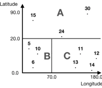
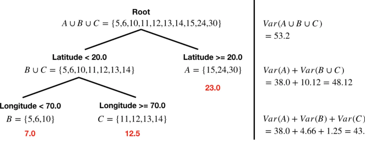
This greedy, top-down, recursive induction process is depicted in Figure 2.5. In the figure,

a dataset is split based on two features (latitude, longitude), with a minimum number of records

per leaf equal to 5, generating a partitioned space with less impurity after each iteration. First,

the dataset starts with a single region A∪B∪C with variance 53.2; then it is split at latitude

equals 20.0 into two regions, top (A) with variance 38.0, and bottom (B∪C) with variance

10.12, leading to a variance of 48.12 after the split. Second, the bottom region is split at

longitude equals 70.0 into another two regions, left (B) with variance 4.66, and right (C) with

variance 1.25, leading to a total variance of 43.91 after the split. Because there are no nodes

left with more than five records, the induction process stops. This spatial partitioning results in

Figure 2.5: Decision Tree region boundaries in a 2-dimensional (latitude, longitude) feature space. Each node in the tree bisects the space into distinct regions.

on the average record values in the leaves. Figure 2.6 shows a view of the resulting tree, with

the node predicates in boldface, node elements in curly brackets, and predictions (A=23, B=7,

C=12.5) at the lower bottom of each leaf.

Random Forests

In order to improve accuracy and reduce overfitting, Ho [33] proposed an ensemble learning

method that utilizes a combination of decision trees, trained on random subsets of the original

feature space, to solve classification, regression, and other tasks. To reach a consensus over the

individual predictions, this ensemble outputs the mode of the classes of the individual trees for

a classification task or the mean of the predictions of the individual trees for a regression task

[33].

Breiman [18] proposed the Random Forest as a method that uses the random subsampling

of the input features (i.e., columns) in tandem with random subsampling of the input data

(i.e., rows), a process known as bagging [16], in order to grow an ensemble of decision trees.

Breiman also proved that bagging these weak learners would result in a more complex model

Figure 2.6: Decision Tree nodes with their predicates in boldface, leaves with their underlying records (described in a set), and predictions at the lower bottom. A summary of the accumu-lated variance after each split is also shown on the right.

way they were trained on random subsets and the way each node had a random set of features

on which it could be split [18].

F(x)= 1

M

M

X

i=1

hi(x) (2.5)

Equation (2.5) relates the output of the bagged ensemble to that from the base learners [18],

whereF(x) is the ensemble output,Mis the number of base learners, andhi(x) is the prediction

of the i-th model given inputx. Furthermore, each hypothesishi(x) is formed by training a base

learner on a random sample ˜N ⊂ N of the original datasetN.

Gradient Boosted Trees

Motivated by Breiman [17], Friedman proposed the Stochastic Gradient Boosting method for

constructing ensembles via a boosting procedure. Stochastic Gradient Boosted Trees (GBT)

[29] differ from Random Forests in that they are sequentially grown by fitting a new tree to the

residuals of the previous one as opposed to grown independently. This sequential dependency

poses difficulties for the training of many decision trees in parallel; however, GBTs can still

be parallelized at the level of a single Decision Tree. Hence, theFindBestSplitfunction can be

aggregated [49].

F0(x)=arg min

γ

N

X

i−1

Ψ(yi, γ) (2.6)

˜

yim= −

"∂Ψ

(yi,Fm−1(xi))

∂Fm−1(xi)

#

,i=1...Ne (2.7)

{Rlm}₁L=terminal nodetree({y˜im,xi}₁Ne) (2.8)

γlm = arg min

γ

X

xi ∈RlmΨ

(yi,Fm−1(xi)+γ) (2.9)

Fm(x)=Fm−1(x)+v∗γlm1(x∈Rlm) (2.10)

Equations (2.6) through (2.10) formally express the GBT boosting process [29], wheremis

the index of the current model, and{yi,xi}₁Neis a random subsample of the training set (Ne< N),

withyirepresenting the i-th record label andxirepresenting the i-th input vector. F0(x) in (2.6)

is the base case of the sequential process, and Ψ is the loss function, typically least squares

in regression problems. ˜yim in (2.7) are the residuals that the current model inherits from the

previous one. Rlm in (2.8) is a set of residuals at disjoint regions (1, . . . ,L) represented by the

tree leaves at iterationm. γlmin (2.9) is the value that minimizes the residuals at leafl. Finally,

in (2.10),vis the learning rate, 1is an indicator function that outputs one ifx ∈Rlm and zero

otherwise, andFm(x) is the final output of the ensemble.

The following are some properties of decision tree ensembles taken from Breiman [18].

1. Relatively robust to outliers and noise.

3. Simple and easily parallelized.

These properties summarize the most important characteristics of the models presented in this

section and point to a means of overcoming the challenges of conducting Machine Learning

over big datasets: parallelization.

2.3.2

Blending Models

Ensemble methods (e.g., bagging, boosting, stacking) train multiple learners in order to solve

a problem. Whereas ordinal learning approaches will train a single model on the dataset,

ensemble methods will train multiple models and weight their contributions to come up with

a final answer [71]. Although there are many different ways of constructing ensembles, (e.g.,

Random Forests are built via bagging), the strategy employed in this work is a special form of

stacking, called blending.

Sill et al. describe stacked models as methods designed to boost predictive accuracy by

blending the predictions of multiple machine learning models [59]. A stacked model is in

itself a meta-model that learns how to weight the contributions of its members based on their

predictions.

Blending is a derived concept introduced by the Netflix prize winners that is very close

to stacked generalization, but more straightforward to implement and safer to guard against

information leaks between the stacker and the generalizers because it keeps a small, completely

separate holdout set to train the stacker [59].

The key to a successful blending is the inclusion of diverse base-learners [59]; where the

diversity in a set of learners can be quantified as a low correlation in their predictions. Hence, in

the context of this work, blending is utilized to enhance the prediction accuracy by combining

2.3.3

Local Learning

Bottou and Vapnik devised what might seem a slow and ineffective way to scale machine

learning algorithms, but one that, in reality, scored, and more importantly scaled, incredibly

well [12]. Noticing that training data are rarely evenly distributed in the input space, Bottou

and Vapnik suggested a change in the typical training process. Instead of relying on a single,

global learner over an entire dataset, they proposed that the training process should rely on

multiple learners trained independently on closely related chunks of data. A simple example

of a local learning algorithm would be as follows [12]. For each testing pattern:

1. Select a few training examples located in the vicinity of the testing pattern.

2. Train any learning model over these few examples.

3. Use that model to predict over the testing pattern.

In particular, local learning provides a construct to scale learning algorithms in terms of

mem-ory, enabling otherwise memory-constrained techniques such as ARIMA to be applied on large

datasets [42][30]. Hence, in the context of this work, local learning is applied with the objective

of scaling time series forecasting models over large geographical regions.

2.3.4

Time-sliding Cross-validation

The aforementioned machine learning models require several hyperparameters in order to be

properly fitted [10]. For example, the maximum depth of the decision tree impacts the

com-plexity of the model, and its value can make the difference between an under-fitted tree and

an over-fitted one. Thus, a fair amount of time is devoted to the tuning of these

hyperparam-eters. Typically, methods such as grid-search and random-search are used in practice [10].

The former performs a train-and-evaluate cycle for all possible combinations of

hyperparam-eters values given as input. The latter conducts a search on the same space randomly and

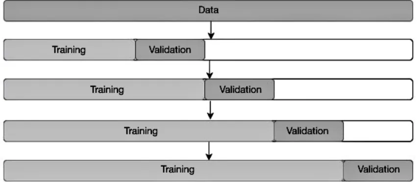
Figure 2.7: Time-sliding window for cross-validation. The Training fold chronologically pre-cedes the validation fold.

Popular methods for evaluating the performance of a machine learning model are

train-validation splits, and cross-train-validation, both of which are often done by picking records at

ran-dom and including them into disjoint training and validation sets. In the Time Series ran-domain,

however, this randomness would wrongly allow the model to be trained on future data, and

as a consequence, to be asked to predict the past [9]. Thus, traditionally in the Time Series

literature out-of-sample methods such as a time-sliding window are utilized to provide a more

accurate evaluation [24]. The process illustrated in Figure 2.7 splits the original training set

into a training set that increases in size for each consecutive fold and a fixed-size validation set

that is slid forward in time to preserve sequentiality.

Forcing the evaluation process to respect the time dimension will likely hurt the model’s

score and running-time performance [9]. However, as a result, the trained model will report

an evaluation metric that is more semantically sound, because the model was never allowed to

peek into the future.

2.4

Distributed Computing And Scalability

Sections 2.3.1 and 2.3.3 offered insights into how the training of tree-based ensembles and

time series forecasting models respectively can be parallelized. This research makes use of

times for machine learning models despite the challenges of Big Data [45][43][14][38].

Distributed computing is a computing paradigm that relies on the communication and

co-ordination of computing systems (i.e., nodes) across a computer network in order to achieve a

common goal [44]. As in parallel computing problems, it is best used when the global goal can

be broken down into independent tasks. For example, the mergesort algorithm has a partition

step that creates independent chunks of data that can later be pair-wise merged into a globally

sorted solution.

Furthermore, the distribution of nodes in a computer network brings additional challenges

in comparison to parallel computing. The abscence of shared memory between nodes means

that they need to communicate by message passing [5]. Figure 2.8 illustrates this memory-wise

difference between distributed computing systems and thread-based parallel systems.

More-over, because messaging over the network can fail, and nodes can also fail, distributed systems

need to be engineered with fault-tolerance in mind [40].

A computing system is deemed horizontally scalable if its computation can be sped up

when distributed across a cluster of machines (i.e., adding a new node reduces the load on the

system). A vertically scalable computing system, however, explores speedups via

improve-ments in the hardware of a single node (i.e., via more expensive hardware with more memory

and processors). Although both techniques have the effect of improving the performance of

a computing system, Michael et al. [46] have demonstrated that scale-out (i.e., horizontal)

solutions offer betterprice/performanceratio than scale-up (i.e., vertical) solutions.

Hence, this research work makes use of distributed computing to offer a cost-effective

scale-out solution that enables unconstrained spatiotemporal forecasting at scale.

2.5

Literature Review

This section reviews the relevant work done by other researchers. It describes successful

shared and diverging aspects concerning this work.

2.5.1

Linear Models

Catlettet al. [20] presented a spatiotemporal forecasting method for predicting crime density

in hot spot regions. The authors pointed out that such information could enable police

de-partments to allocate their limited resources better and develop insightful strategies for crime

prevention. Their proposed approach was made up of two main components: a spatial

cluster-ing partitioner that identifies high-density crime areas, and a collection of multi-variate

auto-regressive models (one per region) that account for the regions discovered in the previous step.

Furthermore, in their implementation, the authors utilize a density-based partitioner (i.e.,

DB-SCAN) for the first component, which resulted in hot spot regions that were diverse in size and

shape. Catlett et al. [20] also demonstrated by means of experiments with public data from

the city of Chicago and New York that their locally learned ARIMA models can outperform

other approaches in the crime forecasting literature. In contrast to their work, this research

partitions the geographical space into square cells of an approximately equal area to facilitate

the forecasting at arbitrary resolutions (e.g., cells with 1m2 _{or 1km}2_area).

Tran et al. [61] proposed a distributed implementation of the spatial regression model

de-vised by Fotheringham et al. [28]. They argued that building a global model over data that

exhibit a spatial relationship could result in misleading global coefficients. For example, a

naive ordinary least-squares regression model trained to predict house prices over an entire

city could learn global coefficients that imply that the older the house, the lower the price.

In fact, there are significant local effects that could indicate that old country houses are more

valuable, possibly because they are reminiscent of an acclaimed architectural style, and old

urban houses tend to be cheaper possibly because they were built with lower construction

stan-dards [28]. The authors then proposed a distributed linear regression method that embedded

the spatial variation of the data in the models’ coefficients [61]. The Geographically Weighted

neighbor-hood of the point in question via a kernel function (e.g., Gaussian) so that points closer to the

point in question have more influence on its value than points that are further away. In synergy

with their work, this research acknowledges the difference between local and global patterns in

the data by training separate models for each. Likewise, it makes use of distributed computing

to train learning models over massive geographical datasets. However, unlike Tranet al. [61],

it explores the use of a feature discretization process before the training of the learning

algo-rithms, and even more importantly, it models both spatial and temporal features as opposed to

only spatial.

Agouaet al.[1] proposed a spatially aware linear regression to predict photovoltaic power

production. Similarly, Cabralet al. [19], and Yadav and Sheoran [67] proposed modifications

to the inner workings of the ARIMA model to deal with spatiotemporal data. In contrast to their

work, this study goes in a different direction, handing offthe spatial responsibilities to another

model, and utilizing pure, locally independent ARIMA models to account for the temporal

component. This separation of concerns was also employed by Andr´eet al. [4], who built a

linear blend, with fixed weights, of Spatiotemporal Vector Autoregressive (STVAR) and Cloud

Motion Vector (CMV) models. In contrast to Andr´e et al., this research utilizes a non-linear

meta-model to learn the weights of the blend as opposed to fixing them.

2.5.2

Neural Networks

Xuet al.[66] proposed a one-step-ahead prediction for taxi demand based on Recurrent Neural

Networks (RNN). The authors claim that many taxi companies still use a naive seasonal average

as their demand forecasting method and argue that sounder methods would enable shorter

waiting times and increased fuel efficiency, translating into cost savings for both drivers and

passengers. Their work leaned on the long-term learning capabilities of the Long-Short Term

Memory (LSTM) networks to model the taxi demand prediction as a sequence forecasting

problem. LSTM networks, which are a type of RNN, contain a memory gating mechanism that

influence its final output. The length of that time window from which past observations are

drawn is called the sequence length and had a fixed value of one week in their experiments

to constraint the computing power required to train the model. Similarly, Huang et al. [34]

proposed an LSTM-based approach for crime prediction while also overcoming the limitations

of the fixed sequence length by using an attention mechanism that enabled the network to pay

more attention to parts of the input sequence. Wanget al. [63] demonstrated another

LSTM-based technique that accounted for spatial sparsity by reducing the geographic plane into a

geographical graph, where nodes were disjoint regions determined by zip-code and edges were

placed according to a statistical process. In contrast to their work, this research relies on time

series models that learn the optimal sequence length during the tuning process and deals with

sparsity by facilitating the use of arbitrary spatial and temporal resolutions.

Liao et al. [41] investigated the use of Deep Neural Networks (DNN), in particular,

ST-ResNet and FLC-Net, to forecast taxi demand. The authors reckoned that the challenges in

making spatiotemporal predictions are caused by strong dependencies in three different realms:

time, space, and external factors (e.g., weather, and holidays). Hence, the DNNs they

exam-ined were selected because their architectures were explicitly designed to deal with both space

and time simultaneously: ST-ResNet [64], which is a weighted blend of Convolution

Neu-ral Networks (CNN) trained on near-term, mid-term, and long-term data; and, FLC-Net [37]

which is a fused Convolutional-LSTM [22] approach, also trained with near, intermediate, and

distant time horizons. Their [41] experimental results, however, surprisingly revealed that the

fusion of models in different temporal horizons had more impact in the results than the specific

choice of DNN, with Feed-Forward networks outperforming all models when such fusion was

not in effect. Moreover, the dependence on convolutional operations resulted in a

computation-ally expensive architecture when dealing with large geographical regions, even after several

optimizations to compact the representation of the data used in the convolution window [41].

The framework proposed in this thesis, however, does not rely on a spatial window to capture

a spatial grid in memory. This representation of the geographical space, akin to an adjacency

list as opposed to a matrix, has lower memory requirements and potentially works better with

sparse data.

Furthermore, to achieve reasonable training times, all the aforementioned neural network

techniques were tested in machines with highly capable GPUs. Due to the high cost of such

hardware, this work favoured techniques that have reasonable training time on CPUs, enabling

the deployment of the proposed framework on cheap commodity hardware, even for

consider-ably large datasets.

2.5.3

Ensemble Models

Reich et al. [52] compiled a seven-year benchmark of influenza forecasts across the United

States. Initially, they commented on how near-real-time forecasts of influenza, fuelled by the

promise of Big Data, could positively impact the public health response to disease outbreaks.

Then they analyzed the performance of twenty-two different models, showing that they

con-sistently outperformed the historical baseline in week-ahead forecasts over multiple influenza

seasons. One important shortcoming that arose in their study was the degradation of the

relia-bility of the forecasts as the prediction horizon became more distant. In other words, in their

experiments, most models became less reliable than the baseline after the forecasting horizon

expanded further than four weeks, leaving public health officials with little time to prepare.

Currently, the proposed research does not contemplate multi-step forecasting and instead

fo-cusses only on the next step, for example, the next hour or the next day, depending on the

required prediction resolution.

Another notable aspect of their work [52] is the performance and stability gains they

achieved by combining several base models into weighted ensembles. Likewise, Ray et al.

[51] also argued that forecasting stability is crucial in any application in the health domain, so

much so that public health officials would favour a trustworthy stable ensemble model over

results [51]. In accordance with their work, this research absorbs this concern for stability and

also relies on a pool of base models as opposed to conceding the forecast responsibility to a

single one. Furthermore, unlike Vanichrujee et al. [62], it uses a blending model to weight

the base learners’ predictions as opposed to a fixed weighting scheme based on the individual

ranked performance of each base model.

Alves et al. [3] demonstrated that tree-based ensembles are highly capable of predicting

crime density at the city level based on socio-economic indicators. Unlike Alves et al. [3],

this research does not directly use such features in its experiments section to keep the results

agnostic of domain features, so that only the merits of spatiotemporal modelling can be

com-pared. However, it leaves the option for users to do so easily in their own experiments. In fact,

the addition of up-to-date domain specific features is expected to lift performance substantially

[3].

2.6

Summary

This chapter has presented a background view of the techniques that support the proposed

framework. It started by describing feature discretization methods pertinent to

spatiotempo-ral datasets. These methods are used by the Spatiotemporal Forecasting Frameworkto build

its representation of temporal and spatial features. It also introduced one of the most popular

time series forecasting models, ARIMA. It also dived into machine learning techniques that

support spatiotemporal forecasting at scale: ensembles of randomly sampled trees; blending

models that promote diversity and stability; a training strategy that allows for the training of

local models; and an evaluation strategy that is suitable for temporal data. These techniques are

what power the multistage machine learning pipeline employed by the Spatiotemporal

Fore-casting Framework. In addition, this chapter portrayed ways in which distributed computing

can help to scale preprocessing and machine learning tasks on top of Big Data. This use of

large volumes of data. Finally, this chapter reviewed the available literature on

spatiotempo-ral forecasting, inspecting techniques based on linear models, neuspatiotempo-ral networks, and ensemble

models in diverse domains. To enable accurate and stable spatiotemporal forecasting at

arbi-trary resolutions despite the challenges posed by Big Data and without the shortcomings of

the reviewed techniques, this research proposes a framework based on a distributed multistage

Spatiotemporal Forecasting Framework

The popularity of smartphones, wearables, IoT, and many other GPS-enabled devices, points

to a future of endless streams of spatiotemporal data arising from diverse knowledge domains.

Machine Learning and Time Series Forecasting emerged as disciplines that could

approx-imate the future value of a given measurement in a dataset and turn it into actionable

infor-mation. The forecasts, however, require the training of learning models on historical data, and

since that amount of data is expected to keep growing following the Big Data trends, it is fitting

to devise a framework that can scale that training.

Hence, the primary objective of this research is to support spatiotemporal forecasts at the

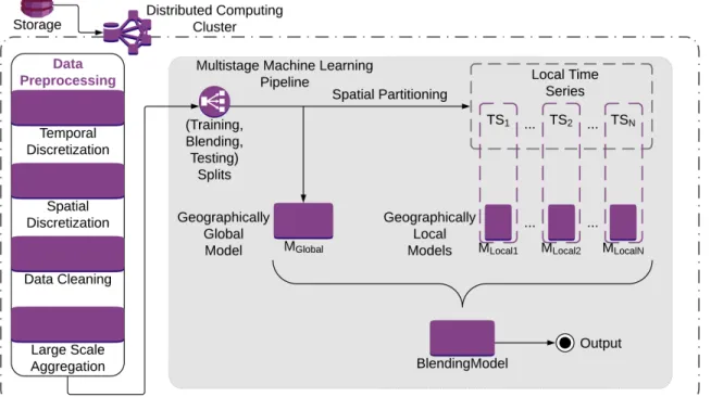
scale of millions of records. To do so, the proposed framework mounts each of its components

on top of a distributed computing backbone, represented in the outer layer of Figure 3.1, which

enables on-demand addition of new machines to handle heavier workloads. In turn, its internal

components also promote parallelism whenever possible, resulting in a system that is highly

horizontally scalable (Section 2.4). Therefore, throughout this chapter, where other viable

techniques existed, this work leaned towards options that conferred more scalability, adhering

to end-to-end scalability by design.

Figure 3.1 illustrates the top-level components of the proposed framework. The goal of

this chapter is to present in detail the inner workings of each component and how they

grate. This chapter is divided as follows: Data Preprocessing, including the discretization,

cleaning, and aggregation processes, and Multistage Machine Learning Pipeline, comprising

the geographically global and local models as well as the blending model.

3.1

Data Preprocessing

This section describes the preprocessing steps that are performed before the data enter the

ma-chine learning pipeline, namely: temporal discretization, spatial discretization, data cleaning,

and large scale aggregation.

Since the essence of this work is to produce forecasts of summaries of events in space and

time, and ultimately to report that information to humans, a discretization of both space and

time is required in order to map a continuous range of values into bins (aggregates or buckets).

The aggregation of values into buckets has the effect of reducing the overall amount of

data and summarizing information into more meaningful chunks [36]. The former reduces the

computing time, and the latter diminishes the cognitive load on the user of the application.

Furthermore, it is worth noting that every preprocessing transformation described in this

section was carefully designed down to the bit level. This low-level optimization is important

since these operations are literally executed millions of times in the preprocessing block.

3.1.1

Temporal Discretization

This work utilizes an Equal Width Discretization (EWD) of the temporal component, a

tech-nique that has been extensively explored in the literature [26] and is directly related to common

temporal aggregates (e.g., day, hour, minute). Discretizing over such fixed width intervals

al-lows the framework to answer forecasting questions that are closer to the cultural norm: for

example, what is the forecasted value for the next hour?

Furthermore, this research work utilizes the Unix Epoch, also known as POSIX Time, to

Original Timestamp Grain String Representation POSIX Time Result Minute 2019/08/08 09:40:00 1565257200 2019/08/08 09:40:40 Hour 2019/08/08 09:00:00 1565254800 Day 2019/08/0800:00:00 1565222400

Table 3.1: Examples of timestamp truncations at arbitrary resolutions.

midnight, January 1st, 1970 (also known as Epoch Zero) and is encoded as a 64-bit integer.

With this encoding, the discretization operation becomes fast to compute since it can be done

via an integer truncation: one integer division followed by one multiplication.

The discretization of a timestamp involves choosing its adequate grain size (also referred

to as resolution), for example, one hour, and then zeroing all finer grains below it: minutes

and seconds. Table 3.1 illustrates the process of truncating an arbitrary timestamp (2019/08/08

09:40:40) to different grain sizes, which can be seen as a transformation that squashes a

contin-uous time interval into a fixed discrete interval. In the table, the 64-bit integer result is obtained

by starting with 1565257240 (the POSIX Time equivalent of the original timestamp) and

per-forming an integer division (i.e., ignores the remainder) by the number of seconds in the grain,

followed by a multiplication by the same factor.

In addition to a fast truncation, the choice of the Unix Time encoding also enables fast

integer-based comparison operations such as filtering and ordering, both of which are of

com-pelling relevance throughout this research.

3.1.2

Spatial Discretization

Whereas an equal width discretization, that squashed a continuous time interval into discrete

temporal bins ordinarily used by humans was possible, a spatial EWD with the same

char-acteristics was not. This impossibility stems from the fact that humans often conquered new

territories through a series of challenging endeavours (e.g., wars, rough terrains), resulting in

geographical regions that broadly vary in shape and size.

Relying on a spatial discretization process based on human-based knowledge would be