Abstract— The conventional method of detection and classification of brain tumor is by human inspection with the use of medical resonant brain images. But it is impractical when large amounts of data is to be diagnosed and to be reproducible. And also the operator assisted classification leads to false predictions and may also lead to false diagnose. Medical Resonance images contain a noise caused by operator performance which can lead to serious inaccuracies classification. The use Support Vector Machine, Kmean and PCA shown great potential in this field. Principal Component Analysis gives fast and accurate tool for Feature Extraction of the tumors. Kmean is used for Image Segmentation. Support Vector Mahine with Training and Testing of Brain Tumor Images techniques is implemented for automated brain tumor classification.
I. INTRODUCTION
A brain tumor or intracranial neoplasm occurs when abnormal cells form within the brain. There are two main types of tumors: malignant or cancerous tumors and benign tumors. Cancerous tumors can be divided into primary tumors that started within the brain and those that spread from somewhere else known as brain metastasis tumors. All types of brain tumors may produce symptoms that vary depending on the part of the brain involved. These may include headaches, seizures, problem with vision, vomiting, and mental changes. The headache is classically worst in the morning and goes away with vomiting. More specific problems may include difficulty in walking, speaking and with sensation. As the disease progresses unconsciousness may occur.
Brain tumors are abnormal and uncontrolled proliferations of cells. Some originate in the brain itself, in which case they are termed primary. Others spread to this location from somewhere else in the body through metastasis, and are termed secondary. Primary brain tumors do not spread to other body sites, and can be malignant or benign. Secondary
brain tumors are always malignant. Both types are potentially disabling and life threatening. Because the space inside the skull is limited, their growth increases intracranial pressure, and may cause edema, reduced blood flow, and displacement, with consequent degeneration, of healthy tissue that controls vital functions. Brain tumors are, in fact, the second leading cause of cancer related deaths in children and young adults. According to the Central Brain Tumor Registry of the United States (CBTRUS), there will be 64,530 new cases of primary brain and central nervous system tumors diagnosed by the end of 2011. Overall more than 600,000 people currently live with the disease.
Brain Anatomy: Nothing in the world can compare with the human brain. This mysterious three-pound organ controls all necessary functions of the body, receives and interprets information from the outside world, and embodies the essence of the mind and soul. Intelligence, creativity, emotion, and memories are a few of the many things governed by the brain.
The brain receives information through our five senses: sight, smell, touch, taste, and hearing - often many at one time. It assembles the messages in a way that has meaning for us, and can store that information in our memory. The brain controls our thoughts, memory and speech, movement of the arms and legs, and the function of many organs within our body. It also determines how we respond to stressful situations (such as taking a test, losing a job, or suffering an illness) by regulating our heart and breathing rate.
Nervous system
The nervous system is divided into central and peripheral systems. The central nervous system (CNS) is composed of the brain and spinal cord. The peripheral nervous system (PNS) is composed of spinal nerves that branch from the spinal cord and cranial nerves that branch from the brain. The PNS includes the autonomic nervous system, which Mr. Arun Kumar (Assistant Prof.), Bhagwan Mahavir Institute Of Engineering & Technology,
Sonepat, [email protected]
A Novel Approach for Brain Tumor Detection
Using Support Vector Machine, K-Means and
PCA Algorithm
Richika, Department of Computer Science and Technology, Bhagwan Mahavir Institute Of
controls vital functions such as breathing, digestion, heart rate, and secretion of hormones.
Skull The purpose of the bony skull is to protect the brain from injury. The skull is formed from 8 bones that fuse together along suture lines. These bones include the frontal, parietal (2), temporal (2), sphenoid, occipital and ethmoid (Fig. 1). The face is formed from 14 paired bones including the maxilla , zygoma, nasal, palatine, lacrimal, inferior nasal conchae, mandible, and vomer.
Figure1. 1. Eight bones form the skull and fourteen bones form the face
Inside the skull are three distinct areas: anterior fossa, middle fossa, and posterior fossa (Fig. 2). Doctors sometimes refer to a tumor‘s location by these terms, e.g., middle fossa meningioma
Figure1. 2. The inside of the skull is divided into three areas called
the anterior, middle, and posterior fossae. Brain: The brain is composed of the cerebrum, cerebellum, and brainstem (Fig. 3).
Figure 1.3. The brain is composed of three parts: the
brainstem, cerebellum, and cerebrum.
The cerebrum is divided into four lobes: frontal, parietal, temporal, and occipital.
The cerebrum is the largest part of the brain and is composed of right and left hemispheres. It performs higher functions like interpreting touch, vision and hearing, as well as speech, reasoning, emotions, learning, and fine control of movement.
The cerebellum is located under the cerebrum. Its function is to coordinate muscle movements, maintain posture, and balance.
The brainstem includes the midbrain, pons, and medulla. It acts as a relay center connecting the cerebrum and cerebellum to the spinal cord. It performs many automatic functions such as breathing, heart rate, body temperature, wake and sleep cycles, digestion, sneezing, coughing, vomiting, and swallowing. Ten of the twelve cranial nerves originate in the brainstem.
The surface of the cerebrum has a folded appearance called the cortex. The cortex contains about 70% of the 100 billion nerve cells. The nerve cell bodies color the cortex grey-brown giving it its name – gray matter (Fig. 4). Beneath the cortex are long connecting fibers between neurons, called axons, which make up the white matter
Figure1. 4. The surface of the cerebrum is called the cortex.
interconnected to other brain areas by axons (white matter). The cortex has a folded appearance. A fold is called a gyrus
and the groove between is a sulcus.
The folding of the cortex increases the brain‘s surface area allowing more neurons to fit inside the skull and enabling higher functions. Each fold is called a gyrus, and each groove between folds is called a sulcus. There are names for the folds and grooves that help define specific brain regions.
A. Right brain – left brain
The right and left hemispheres of the brain are joined by a bundle of fibers called the corpus callosum that delivers messages from one side to the other. Each hemisphere controls the opposite side of the body. If a brain tumor is located on the right side of the brain, your left arm or leg may be weak or paralyzed.
Not all functions of the hemispheres are shared. In general, the left hemisphere controls speech, comprehension, arithmetic, and writing. The right hemisphere controls creativity, spatial ability, artistic, and musical skills. The left hemisphere is dominant in hand use and language in about 92% of people.
B. Lobes of the brain
The cerebral hemispheres have distinct fissures, which divide the brain into lobes. Each hemisphere has 4 lobes: frontal, temporal, parietal, and occipital (Fig 3). Each lobe may be divided, once again, into areas that serve very specific functions. It‘s important to understand that each lobe of the brain does not function alone. There are very complex relationships between the lobes of the brain and between the right and left hemispheres.
1) Frontal lobe
Personality, behavior, emotions Judgment, planning, problem solving Speech: speaking and writing (Broca‘s area) Body movement (motor strip)
Intelligence, concentration, self awareness
2) Parietal lobe
Interprets language, words
Sense of touch, pain, temperature (sensory strip)
Interprets signals from vision, hearing, motor, sensory and memory
Spatial and visual perception
3) Occipital lobe
Interprets vision (color, light, movement)
4) Temporal lobe
Understanding language (Wernicke‘s area) Memory
Hearing
Sequencing and organization
Messages within the brain are carried along pathways. Messages can travel from one gyrus to another, from one lobe to another, from one side of the brain to the other, and to structures found deep in the brain (e.g. thalamus, hypothalamus).
Brain tumor:
A brain tumor is a mass or growth of abnormal cells in your brain.
Many different types of brain tumors exist. Some brain tumors are noncancerous (benign), and some brain tumors are cancerous (malignant). Brain tumors can begin in your brain (primary brain tumors), or cancer can begin in other parts of your body and spread to your brain (secondary, or metastatic, brain tumors).
Brain tumor treatment options depend on the type of brain tumor you have, as well as its size and location.
The signs and symptoms of a brain tumor vary greatly and depend on the brain tumor's size, location and rate of growth.
General signs and symptoms caused by brain tumors may include:
New onset or change in pattern of headaches Headaches that gradually become more frequent and more severe
Unexplained nausea or vomiting
Vision problems, such as blurred vision, double vision or loss of peripheral vision
Gradual loss of sensation or movement in an arm or a leg Difficulty with balance
Speech difficulties
Confusion in everyday matters Personality or behavior changes
Seizures, especially in someone who doesn't have a history of seizures
Hearing problems
5) 1.3.1 Brain tumors that begin in the brain (Primary):
Primary brain tumors begin when normal cells acquire errors (mutations) in their DNA. These mutations allow cells to grow and divide at increased rates and to continue living when healthy cells would die. The result is a mass of abnormal cells, which forms a tumor.
Primary brain tumors are much less common than are secondary brain tumors, in which cancer begins elsewhere and spreads to the brain.
Many different types of primary brain tumors exist. Each gets its name from the type of cells involved. Examples include:
Acoustic neuroma (schwannoma)
Astrocytoma, also known as glioma, which includes anaplastic astrocytoma and glioblastoma
Ependymoma
Germ cell tumor Medulloblastoma
Meningioma
Oligodendroglioma Pineoblastoma
6) 1.3.2 Cancer that begins elsewhere and spreads to the brain (Secondary)
Secondary (metastatic) brain tumors are tumors that result from cancer that starts elsewhere in your body and then spreads (metastasizes) to your brain.
Secondary brain tumors most often occur in people who have a history of cancer. But in rare cases, a metastatic brain tumor may be the first sign of cancer that began elsewhere in your body.
Secondary brain tumors are far more common than are primary brain tumors.
Any cancer can spread to the brain, but the most common types include:
Breast cancer Colon cancer Kidney cancer Lung cancer Melanoma
Risk Factors:
Though doctors aren't sure what causes the genetic mutations that can lead to primary brain tumors, they've identified factors that may increase your risk of a brain tumor. Risk factors include:
1. Your age: Your risk of a brain tumor increases as you age. Brain tumors are most common in older adults. However, a brain tumor can occur at any age. And certain types of brain tumors occur almost exclusively in children. 2. Exposure to radiation: People who have been exposed to a type of radiation called ionizing radiation have an increased risk of brain tumor. Examples of ionizing radiation include radiation therapy used to treat cancer and radiation exposure caused by atomic bombs.
3. More common forms of radiation, such as electromagnetic fields from power lines and radiofrequency radiation from cellphones and microwave ovens, have not been proved to be linked to brain tumors.
4. Family history of brain tumors. A small portion of brain tumors occur in people with a family history of brain tumors or a family history of genetic syndromes that increase the risk of brain tumors.
Test and Diagnosis
If it's suspected that you have a brain tumor, your doctor may recommend a number of tests and procedures, including:
1. A neurological exam. A neurological exam may include, among other things, checking your vision, hearing, balance, coordination and reflexes. Difficulty in one or more areas may provide clues about the part of your brain that could be affected by a brain tumor.
2. Imaging tests. Magnetic resonance imaging (MRI) is commonly used to help diagnose brain tumors. In some cases a dye may be injected through a vein in your arm before your MRI.
3. A number of specialized MRI scans — including functional MRI, perfusion MRI and magnetic resonance spectroscopy — may help your doctor evaluate the tumor and plan treatment.
4. Other imaging tests may include computerized tomography (CT) scan and positron emission tomography (PET).
5. Tests to find cancer in other parts of your body. If it's suspected that your brain tumor may be a result of cancer that has spread from another area of your body, your doctor may recommend tests and procedures to determine where the cancer originated. One example might be a CT scan of the chest to look for signs of lung cancer.
6. Collecting and testing a sample of abnormal tissue (biopsy). A biopsy can be performed as part of an operation to remove the brain tumor, or a biopsy can be performed using a needle.
skull. A thin needle is then inserted through the hole. Tissue is removed using the needle, which is frequently guided by CT or MRI scanning.
8. The biopsy sample is then viewed under a microscope to determine if it is cancerous or benign. This information is helpful in guiding treatment.
Problem Definition
The boundary of the tumor in an image is usually traced by hand which is time consuming and difficult to detect and localize, detection becomes infeasible with large set of data sets.
While typically dealing with medical images where pre-surgery and post surgery decisions are required for the purpose of initiating and speeding up the recovery process.
Manual segmentation of abnormal tissues cannot be compared with modern day‘s high speed computing machines which enable us to visually observe the volume and location of unwanted tissues. Hence there is a need for the automatic system for the detection of tumor.
II. RELATED WORK
Meenakshi Sharma, Simranjit Singh et.al.[1] The precise information of a tumor plays an important role in the treatment of malignant tumors. The manual segmentation of brain tumors from Magnetic Resonance images (MRI) is time consuming task. Processing of MRI images is one of the parts of this field. The detection and extraction of tumor is done from patient‘s MRI scan images of the brain. The basic concepts of the image processing are some noise removal functions, segmentation and morphological operations. The modified image segmentation and histogram thresh holding techniques were applied on MRI scan images in order to detect brain tumors. In addition, a region prop and skull is used to detect the tumor in the brain. The proposed method can be successfully applied to detect the contour of the tumor and its geometrical dimension. The result of proposed research has been very promising
K.Selvanayaki , Dr.P.Kalugasalam et.al.[2] The Segmentation is a fundamental technique used in image processing to extract suspicious regions from the given image. In this paper proposes the meta-heuristic methods such as Ant Colony optimization (ACO), genetic algorithm (GA) and Particle swarm optimization (PSO) for segmenting brain tumors in 3D magnetic resonance images. Here this paper is divided into two stages. In the first stage preprocessing and enhancement is performed using tracking algorithms. These are used to preprocessing to suppress artifacts, remove unwanted skull portions from brain MRI
and these images are enhanced using weighted median filter. The enhanced technique is evaluated by Particle swarm optimization (PSNR) and Average Signal-to-Noise Ratio (ASNR) for filters. In the Second stage of the intelligent segmentation is three algorithms will be implemented for identifying and segmenting of suspicious region using ACO, GA and PSO, and their performance is studied. The proposed algorithms are tested with real patients MRI. Results obtained with a brain MRI indicate that this method can improve the sensitivity and reliability of the systems for automated detection of brain tumors .The algorithms are tested on 21 pairs of MRI from real patient‗s brain database and evaluate the performance of the proposed method. T. Logeswari and M. Karnan et.al.[3] Image segmentation is an important and challenging factor in the medical image segmentation. This paper describes segmentation method consisting of two phases. In the first phase, the MRI brain image is acquired from patients‘ database, In that film, artifact and noise are removed after that HSom is applied for image segmentation. The HSom is the extension of the conventional self organizing map used to classify the image row by row. In this lowest level of weight vector, a higher value of tumor pixels, computation speed is achieved by the HSom with vector quantization. Roopali R.Laddha, S.A.Ladhake et.al.[4] —The brain is the anterior most part of the central nervous system. The location of tumors in the brain is one of the factors that determine how a brain tumor effects an individual's functioning and what symptoms the tumor causes. Along with the Spinal cord, it forms the Central Nervous System (CNS). Brain tumor is an abnormal growth caused by cells reproducing themselves in an uncontrolled manner. Magnetic Resonance Imager (MRI) is the commonly used device for diagnosis. In MR images, the amount of data is too much for manual interpretation and analysis. During past few years, brain tumor segmentation in magnetic resonance imaging (MRI) has become an emergent research area in the field of medical imaging system. Accurate detection of size and location of brain tumor plays a vital role in the diagnosis of tumor. An efficient algorithm is proposed for tumor detection based on segmentation and morphological operators. Firstly quality of scanned image is enhanced and then morphological operators are applied to detect the tumor in the scanned image. We also propose an efficient wavelet based algorithm for tumor detection which utilizes the complementary and redundant information from the Computed Tomography (CT) image and Magnetic Resonance Imaging (MRI) images. Hence this algorithm effectively uses the information provided by the CT image and MRI images there by providing a resultant fused image which increases the efficiency of tumor detection.
then morphological operators are applied to detect the tumor in the scanned image.
Mandhir Kaur and Dr. Rinkesh Mittal et.al.[6] This review paper surveys some primary and critical research question of the methods that involve non-invasive approach for detection of brain tumor using image processing techniques and the main question whether the process can be webified with intelligence algorithm. This paper includes a study of recent state of art technologies, techniques and algorithms used in tumor detection. This paper discusses and summarises the issues related to validity of these methods as well their performance. Exhaustive lists of machine learning algorithms that have been used for this purpose have been examined for the reason and importance of their use for tumor detection. Then one of the section the quality and quantity of the image dataset which has been used have been surveyed, question like whether real type of cases or simulated cases have been used to build the premises and thesis of research work have also been examined from papers solicited on this particular topic, this too has also been done questioning the relevance, significance of features being used in tumor detection. Above all, we have examined how this system can be part of new technologies like cloud with intelligence.
Kimmi Verma , Aru Mehrotra , Vijayeta Pandey , Shardendu Singh et.al.[7] Brain tumor analysis is done by doctors but its grading gives different conclusions which may vary from one doctor to another. So for the ease of doctors, a research was done which made the use of software with edge detection and segmentation methods, which gave the edge pattern and segment of brain and brain tumor itself. Medical image segmentation had been a vital point of research, as it inherited complex problems for the proper diagnosis of brain disorders. In this research, it provides a foundation of segmentation and edge detection, as the first step towards brain tumor grading. Current segmentation approaches are reviewed with an emphasis placed on revealing the advantages and disadvantages of these methods for medical imaging applications. The use of image segmentation in different imaging modalities is also described along with the difficulties encountered in each modality.
Gauri P. Anandgaonkar , Ganesh.S.Sable et.al.[8] Brain tumor is an uncontrolled growth of tissues in human brain. This tumor, when turns in to cancer become life-threatening. So medical imaging, it is necessary to detect the exact location of tumor and its type. For locating tumor in magnetic resonance image (MRI) segmentation of MRI plays an important role. This paper includes survey on different segmentation techniques applied to MR Images for locating tumor. It also includes a proposed method for the same using Fuzzy C-Means algorithm and an algorithm to find area of tumor which is usefull to decide type of brain tumor.
Mr. R. G. Selkar , Prof. M. N. Thakare , Prof. B. J. Chilke et.al.[9] The main objective is to detect and segment the brain tumor using watershed and thresholding algorithm. Brain tumor segmentation in magnetic resonance imaging (MRI) has become an emergent research area in the field of
medical imaging system. Brain tumor detection helps in finding the exact size, shape, boundary extraction and location of tumor. The system will consist of three stages to detect and segment a brain tumor. An efficient algorithm will proposed for tumor detection based on segmentation and morphological operators. Firstly quality of scanned image will enhanced and then morphological operators will be applied to detect the tumor in the scanned image. To improve the quality of images and limit the risk of distinct regions fusion in the segmentation phase an enhancement process will be applied. It will be simulate on Matlab Software.
Sneha Khare, Neelesh Gupta, Vibhanshu Srivastava et.al.[10] This paper proposes an approach to detect tumor present in the brain. Tumor is an abnormal and uncontrolled division of cells. Proposed method is based on Genetic Algorithm and Curve Fitting to segment the MRI image. The Support Vector Machine has been used to classify the tumorous and nontumorous image. Finally, the tumor will be detected by extracting the features of segmented image which is being classified using Support Vector Machine. The algorithm has attempted to achieve 98% of accuracy in detecting the tumor in brain.
2.1 Literature review on Principal Component Analysis: Abstract: Feature extraction is a method of capturing visual content of an image. The feature extraction is the process to represent raw image in its reduced form to facilitate decision making such as pattern classification. We have tried to address the problem of classification MRI brain images by creating a robust and more accurate classifier which can act as an expert assistant to medical practitioners. The objective of this paper is to present a novel method of feature selection and extraction. This approach combines the Intensity, Texture, shape based features and classifies the tumor as white matter, Gray matter, CSF, abnormal and normal area. The experiment is performed on 40 tumor contained brain MR images from the Internet Brain Segmentation Repository. The proposed technique has been carried out over a larger database as compare to any previous work and is more robust and effective.. PCA method is used to reduce the number of features used. The feature selection using the proposed technique ismore beneficial as it analyses the data according to grouping class variable and gives reduced feature set with high classification accuracy.
Principal Component Analysis (PCA): Principal components are the projection of the original features onto the eigenvectors and correspond to the largest eigenvalues of the covariance matrix of the original feature set. Principle components provide linear representation of the original data using the least number of components with the mean squared error minimized PCA can be used to approximate the original data with lower dimensional feature vectors. The basic approach is to compute the eigenvectors of the covariance matrix of the original data, and approximate it by a linear combination of the leading eigenvectors. By using PCA procedure, the test image can be identified by first, projecting the image onto the eigen space to obtain the corresponding set of weights, and then comparing with the set of weights of the faces in the training set.
For the diagnostic process in pathology, we can discern two main steps. First pathologists observe tissue and recognize certain histological attributes related to the degree of tumor malignancy. In a second step interpret their histological findings and come up with a decision related to tumor grade. In most of the cases, pathologists are unaware of precisely how many attributes have been considered in their decision but they are able to classify tumors almost instantly and unconscious of the complexity of the task performed. Pathologists are capable to verbalize their impression of particular features. For example, they can call mitosis and apoptosis as ―present‖ or ―absent‖ but they do not know how precisely these concepts have to be taken into account in the decision process. To this end, although the same set of features is recognized by different histopathologists, each one is likely to reach to a different diagnostic output. To confine subjectivity, considerable efforts have been made based on computer-assisted methods with a considerable high level of accuracy. It proposes data-driven grading models such as statistical vector machines, artificial neural networks, and decision trees coupled with image analysis techniques to incorporate quantitative histological features. However, besides the retention and enhancement of achieved diagnostic accuracies in supporting medical decision, one of the main objectives, is to enlarge the inter-operability and increase transparency in decision-making. The latter is major importance in clinical practice, where a premium is placed on the reasoning and comprehensibility of consulting systems.
Review on Clustering:
In fact, most of the segmentation algorithms proposed so far are based on classification or clustering approaches. This is mostly owed to the fact that with these methods, multi-modal datasets can be handled easily because they can operate on any chosen feature vector. In most cases, the features on which these algorithms operate include voxel-wise intensities and frequently also local textures. The general idea is to decide for every single voxel individually to which class it belongs based on its feature vector. Classification requires training data to learn a classification model, based on which new instances can be labeled.
Clustering, on the other hand, works in an unsupervised way and groups data based on certain similarity criteria [11]. Clustering was introduced into the brain tumor segmentation community by Schad et al [12] who analyzed texture patterns of different tissues. Phillipset et al [13] employed fuzzy c-means clustering and Vaidyanathan [14] compared this to kNN clustering for the tumor volume determination during therapy on multi-spectral 2D image slices. Clark et al [15], from the same group, further developed this approach to incorporate knowledge-based techniques. Later, Fletcher-Heath et al [16] also combined fuzzy clustering with knowledge-based techniques for the brain tumor segmentation from multi-sequence MRI.
Comparison of classification and clustering methods
III. PROPOSED SYSTEM
We proposed a method with quantization process using PCA for images and will focus on clustering process of different detecting areas of the brain and finally with ROI technique we will detect the brain tumor and image will reflect the segmented portion of brain tumor
Proposed Method For Brain Tumor Detection
Figure3.1: Proposed system Architecture
Segmentation of Brain Tumor Using Principal Component Analysis
Abstract: The conventional method of detection and classification of brain tumor is by human inspection with the use of medical resonant brain images. But it is impractical when large amounts of data are to be diagnosed and to be reproducible. And also the operator assisted classification leads to false predictions and may also lead to false diagnose. Medical Resonance images contain a noise caused by operator performance which can lead to serious inaccuracies classification. The use of artificial intelligent techniques for instant, neural networks, and fuzzy logic shown great potential in this field. Statistical Principal Component Analysis gives fast and accurate classification and is a best tool for classification of the tumors. Probabilistic Neural Network with image and data processing techniques is implemented for automated brain tumor classification. The performance of PCA was evaluated in terms of training performance and classification accuracies.
Introduction:
PCA was invented in 1901 by Karl Pearson, as an analogue of the principal axes theorem in mechanics; it was later independently developed (and named) by Harold Hotelling in the 1930s. The method is mostly used as a tool in exploratory data analysis and for making predictive models. PCA can be done by eigenvalue decomposition of a data covariance (or correlation) matrix or singular value decomposition of a data matrix, usually after mean centering (and normalizing or using Z-scores) the data matrix for each attribute. The results of a PCA are usually discussed in terms of component scores, sometimes called factor scores (the transformed variable values corresponding to a particular data point), and loadings (the weight by which each standardized original variable should be multiplied to get the component score).
Authors Modalities Method Accuracy Schad et al(1993) T1, T2 Texture
analysis and clustering
Phillips et al(1995) T1, T2, PD Clustering
Vaidyanathan (1995)
T1, T2, PD Clustering
Clark et al(1998) T1, T2, PD
Knowledge-based techniques
0.69–0.99 (% match) Fletcher-Heath T1, T2, PD Fuzzy
clustering + knowledge-
0.53–0.91 (% match)
et al (2001) based techniques
Cai et al(2007) T1, T1c, T2,
T2flair, DTI
Probabilistic segmentation
0.73–0.98 (classification rate)
based on
multi-modality MRI
Ruan et al(2007) T1, T2,
T2flair, PD
SVM classification
0.99 (TP) Verma et al(2008) T1, T1c, T2,
T2flair, DTI
Multi-parametric
0.34–0.93 (classification rate)
tissue
classification Jensen and T1, T1c, T2,
T2flair,
Different classifiers on
0.78–0.86 (overlap) Schmainda (2009) DWI, DTI,
DSC
multi-parametric MRI
Ruan et al(2011) T2, T2flair,
PD
Image fusion for the
PCA is the simplest of the true eigenvector-based multivariate analyses. Often, its operation can be thought of as revealing the internal structure of the data in a way that best explains the variance in the data. If a multivariate dataset is visualised as a set of coordinates in a high-dimensional data space (1 axis per variable), PCA can supply the user with a lower-dimensional picture, a projection or "shadow" of this object when viewed from its (in some sense; see below) most informative viewpoint. This is done by using only the first few principal components so that the dimensionality of the transformed data is reduced. PCA is closely related to factor analysis. Factor analysis typically incorporates more domain specific assumptions about the underlying structure and solves eigenvectors of a slightly different matrix.
PCA is also related to canonical correlation analysis (CCA). CCA defines coordinate systems that optimally describe the cross-covariance between two datasets while PCA defines a new orthogonal coordinate system that optimally describes variance in a single dataset.[6][7]
PCA is a mathematical procedure that uses an orthogonal transformation to convert a set of observations of possibly correlated variables into a set of values of linearly uncorrelated variables called principal components. The number of principal components is less than or equal to the number of original variables. This transformation is defined in such a way that the first principal component has the largest possible variance (that is, accounts for as much of the variability in the data as possible), and each succeeding component in turn has the highest variance possible under the constraint that it be orthogonal to (i.e., uncorrelated with) the preceding components. Principal components are guaranteed to be independent only if the data set is jointly normally distributed. PCA is sensitive to the relative scaling of the original variables. Depending on the field of application, it is also named the discrete Karhunen–Loève transform (KLT), the Hotelling transform or proper orthogonal decomposition (POD).
Steps:
Convert the 2D images into one dimensional image using reshape function-for both test image and database images.
Find the mean value for each one dimensional image by dividing sum of pixel values and number of pixel values.
Find the difference matrix for each images by [A]=(Original pixel intensity of 1D image) – (mean value)
Find the covariance matrix L
Find the Eigen vector for 1D image V, By using this, get the Vector and diagonal matrix of the 1D images.
Find the Eigen face of 1D image,
By using these principal components, we can identify the image from database which is similar to the features of test image.
It is a way of identifying patterns in data, and expressing the data in such a way as to highlight their similarities and differences. Since patterns in data can be hard to find in data of high dimension, where the luxury of graphical representation is not available, PCA is a powerful tool for analysing data.
The other main advantage of PCA is that once you have found these patterns in the data, and you compress the data, i.e. by reducing the number of dimensions, without much loss of information.
Feature Extractions and Classification
This problem has been broadly dealt under the subject area of 'Pattern Recognition.' The main aim of pattern recognition is the classification of patterns and sub-patterns in an image or scene (Duda, et al., 2001). A pattern recognition system includes the following subsystems: subsystem to define pattern/texture class, subsystem to extract selected features, and subsystem for classification known as classifier (Jain et al., 2000).The pattern classes are normally defined in supervised mode; after this, the desired features are extracted by feature-extracting subsystem, and finally classification is done on the basis of extracted features by classifier. The three main approaches of pattern recognition for feature extraction and classification based on the type of features are as follows: 1) statistical approach, 2) syntactic or structural approach, and 3) spectral approach. In case of statistical approach, pattern/texture is defined by a set of statistically extracted features represented as vector in multidimensional feature space. The statistical features could be based on first-order, second-order, or higher-order statistics of gray level of an image. The feature vector so generated from patterns is assigned to their specific class by probabilistic or deterministic decision algorithm (Fukunaga, 1990).In case of syntactic approach, texture is defined by texture primitives, which are spatially organized according to placement rules to generate complete pattern. In syntactic pattern recognition, a formal analogy is drawn between the structural pattern and the syntax of language (Pavilidis, 1980). In case of spectral method, textures are defined by spatial frequencies and are evaluated by autocorrelation function of a texture. As a comparison between the above-mentioned three approaches, spectral frequency-based methods are less efficient, while statistical methods are particularly useful for random patterns/textures; while for complex patterns, syntactic or structural methods give better results.
syntactic and statistical approaches for texture-based segmentation and classification with artificial neural network (ANN) as segmentation and classifier tool. In this scheme, we have used first- and second-order statistical features of the texture-primitive cell for segmentation and classification. In contrast with the syntactic approach, instead of using rules and grammar to represent pattern in terms of sentences, we used analysis by synthesis method (Tomito et al., 1982). The image is re-synthesized on the basis of classification data produced by ANN. The location and size of texture to be segmented and classified can be directly seen. We have designed and developed an algorithm for analysis of medical images based on hybridization of syntactic and statistical approaches, using artificial neural network (ANN).
The textural properties have been derived using: 1) First-order statistics and 2) Second-First-order statistics that are computed from spatial gray-level co-occurrence matrices (GLCMs).
First order statistical features: They are also called as amplitude or histogram features as they are computed indirectly in terms of the histogram of image pixels within a neighborhood. The statistical moments are calculated from the first order gray-level histogram, which is defined as the distribution of the probability of occurrence of a gray level in the image (Gonzalez and Woods, 2004).
Let z be a random variable denoting gray levels and let p(zi) , i = 0, 1, 2,…., L– 1, be the corresponding
histogram, where L is the number of distinct gray levels. The
nth moment of z about the mean is given by:
iL
i
n i
n
z
z
m
p
z
10
The different parameters that are computed by using statistical moments are:
Mean ,
Standard deviation , Smoothness and Skew-ness.
In addition to the above four parameters, two other parameters are calculated from the first order histogram. They are:
Uniformity and Entropy .
Mean:
The mean just tells us the average gray level of each region and is gives us only a rough idea about the intensity, not really texture.
iL
i
i
p
z
z
m
10
Standard Deviation:
The standard deviation is much more informative, it indicates the variability of gray levels i.e., change in the contrast.
i
iL
i
z
p
.
m
z
21
0
Smoothness:
It measures the relative smoothness of the intensity in a region. This equals to 0 for a region of constant intensity and approaches 1 for regions with large variability in the values of its intensity levels.
2
1
1
1
R
Skewness:
This is calculated from the 3rd statistical moment. The third moment is useful for determining the degree of symmetry of histograms and whether they are skewed to the left (negative value) or right (positive value). This gives a rough idea of whether the gray levels are biased toward the dark or light side of the mean. In terms of texture, the information derived from the third moment is useful only when variations between measurements are large.
10
3 3
L
i
i i
m
p
z
z
Uniformity:
10 2
L
i
i
z
p
U
Entropy:
It is a measure of randomness, image with equalized histogram is having higher entropy i.e. pixels are equally occupying the gray levels; on the other hand if lesser gray levels are occupied (for example incase of thresholded image) image entropy is low.
10
2
L
i
i i
log
p
z
z
p
e
Note: These functions can provide useful information about the texture of an image but cannot provide information about shape, i.e., the spatial relationships of pixels in an image. Another statistical method that considers the spatial relationship of pixels is the gray-level co-occurrence matrix (GLCM), also known as the spatial gray-level dependence matrix.
Method
Step 1: Get some data
In my simple example, I am going to use my own made-up data set. It‘s only got 2 dimensions, and the reason why I have chosen this is so that I can provide plots of the data to show what the PCA analysis is doing at each step
Step 2: Subtract the mean
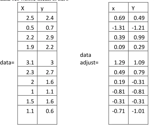
For PCA to work properly, you have to subtract the mean from each of the data dimensions. The mean subtracted is the average across each dimension. So, all the values have (the mean of the values of all the data points) subtracted, and all the values have subtracted from them. This produces a data set whose mean is zero
X y x Y
2.5 2.4 0.69 0.49
0.5 0.7 -1.31 -1.21
2.2 2.9 0.39 0.99
1.9 2.2 0.09 0.29
data= 3.1 3
data
adjust= 1.29 1.09
2.3 2.7 0.49 0.79
2 1.6 0.19 -0.31
1 1.1 -0.81 -0.81
1.5 1.6 -0.31 -0.31
1.1 0.6 -0.71 -1.01
Figure 3.2 Original data
Figure3.3 Data adjust Step 3: Calculate the covariance matrix
Since the data is 2 dimensional, the covariance matrix will be There are no surprises here, so I will just give you the result
Cov=(0.616655 0.615444;0.615444 0.716555) So, since the non-diagonal elements in this covariance matrix are positive, we should expect that both the and variable increase together.
Step 4: Calculate the eigenvectors and eigenvalues of the covariance matrix
Since the covariance matrix is square, we can calculate the eigenvectors and eigenvalues for this matrix. These are rather important, as they tell us useful information about our data. I will show you why soon. In the meantime, here are the eigenvectors and eigenvalues:
Eigen values=(0.49083; 1.28402)
Eigen vectors=(0.735178 0.677873; 0.6778773 -0.735178)
It is important to notice that these eigenvectors are both unit
have plotted both the eigenvectors as well. They appear as diagonal dotted lines on the plot. As stated in the eigenvector section, they are perpendicular to each other. But, more importantly, they provide us with information about the patterns in the data. See how one of the eigenvectors goes through the middle of the points, like drawing a line of best fit? That eigenvector is showing us how these two data sets are related along that line. The second eigenvector gives us the other, less important, pattern in the data, that all the points follow the main line, but are off to the side of the main line by some amount. So, by this process of taking the eigenvectors of the covariance matrix, we have been able to extract lines that characterise the data. The rest of the steps involve transforming the data so that it is expressed in terms of them lines.
Step 5: Choosing components and forming a feature vector:
Here is where the notion of data compression and reduced dimensionality comes into it.
eigenvalues are quite different values. In fact, it turns out that the eigenvector with the highest eigenvalue is the
principle component of the data set. In our example, the eigenvector with the larges eigenvalue was the one that pointed down the middle of the data. It is the most significant relationship between the data
dimensions. In general, once eigenvectors are found from the covariance matrix, the next step is to order them by eigenvalue, highest to lowest. This gives you the components in order of significance. Now, if you like, you can decide to ignore the components of lesser significance. You do lose some information, but if the eigenvalues are small, you don‘t lose much. If you leave out some components, the final data set will have less dimensions than the original. To be precise, if you originally have dimensions in your data, and so you calculate eigenvectors and eigenvalues, and then you choose only the first eigenvectors, then the final data set has only dimensions. What needs to be done now is you need to form a feature vector, which is just a fancy name for a matrix of vectors. This is constructed by taking the eigenvectors that you want to keep from the list of eigenvectors, and forming a matrix with these eigenvectors in the columns.
Step 6: Deriving the new data set
This the final step in PCA, and is also the easiest. Once we have chosen the components (eigenvectors) that we wish to keep in our data and formed a feature vector, we simply take the transpose of the vector and multiply it on the left of the original data set transposed.
Where is the matrix with the eigenvectors in the columns
transposed so that the eigenvectors are now in the rows, with the most significant eigenvector at the top, and is the mean-adjusted data transposed, ie. the data items are in each column, with each row holding a separate dimensions easier if we take the transpose of the feature vector and the data first, rather that having a little T symbol above their names from now on is the final data set, with data items in columns, and dimensions along rows. What will this give us? It will give us the original data solely in terms of the vectorswe chose. Our original data set had two axes and so
our data was in terms of them. It is possible to express data in terms of any two axes that you like. If these axes are perpendicular, then the expression is the most efficient. This was why it was important that eigenvectors are always perpendicular to each other. We have changed our data from being in terms of the axes and now they are in terms of our 2 eigenvectors. In the case of when the new data set has reduced dimensionality, ie We have left some of the eigenvectors out, the new data is only in terms of the vectors that we decided to keep.
To show this on our data, I have done the final transformation with each of the possible feature vectors. I have taken the transpose of the result in each case to bring the data back to the nice table-like format. I have also plotted the final points to show how they relate to the components. In the case of keeping both eigenvectors for the transformation, we get the data and the plot found in Figure 3.3. This plot is basically the original data, rotated so that the eigenvectors are the axes. This is understandable since we have lost no information in this decomposition.
The other transformation we can make is by taking only the eigenvector with the largest eigenvalue. The table of data resulting from that is found in Figure 3.4. As expected, it only has a single dimension. If you compare this data set with the one resulting from using both eigenvectors, you will notice that this data set is exactly the first column of the other. So, if you were to plot this data, it would be 1 dimensional, and would be points on a line in exactly the positions of the points in the plot in Figure 3.3. We have effectively thrown away the whole other axis, which is the other eigenvector. So what have we done here? Basically we have transformed our data so that is expressed in terms of the patterns between them, where the patterns are the lines that most closely describe the relationships between the data. This is helpful because we have now classified our data point as a combination of the contributions from each of those lines. Initially we had the simple and axes. This is fine, but the and values of each data point don‘t really tell us exactly how that point relates to the rest of the data. Now, the values of the data points tell us exactly where (ie. above/below) the trend lines the data point sits. In the case of the transformation using both eigenvectors,
we have simply altered the data so that it is in terms of those eigenvectors instead of the usual axes. But the single-eigenvector decomposition has removed the contribution due to the smaller eigenvector and left us with data that is only in terms of the other.
Relation between PCA and K-Means:
Segmentation of Medical Images Using K-mean Clustering
Abstract: The present Chapter provides a methodology for fully automated K-mean clustering algorithm method for segmentation of medical images. The approach is based on unsupervised segmentation of ima. Experimentation has been carried out on more than 180 MR and CT images for different values of these parameters. On the basis of results, the best-suited value of these parameters has been suggested for accurate segmentation of different types of medical images. Finally, the algorithm has been tested on different types of DICOM format medical images of different body parts and an overall correct segmentation of 97% has been achieved. The results have been evaluated by radiologists and are of clinical importance for segmentation and classification of Region of Interest (ROI). There are dissimilar types of algorithm were developed for brain tumor detection. But they may have some drawback in detection and extraction. After the segmentation, which is done through k-means clustering and fuzzy c-means algorithms the brain tumor is detected and its exact location is identified. Comparing to the other algorithms the performance of fuzzy c-means plays a major role.
Introduction: Segmentation and classification algorithms can be divided into two broad categories: (a) supervised and (b) unsupervised. In the supervised category, most of the classifier algorithms require extensive supervision and training. Unsupervised algorithms are mostly clustering based and are independent of training method and training data. In order to compensate for the lack of training data, clustering methods iterate between segmenting the image and characterizing the properties of the each class. In a sense, clustering methods train themselves using the available data. A functional definition of clusters states that, Patterns within a cluster are more similar to each other than patterns belonging to different clusters (Jain et al. 2000). Two commonly used clustering algorithms are the K-means or hard c-means algorithm (Bezdek et al., 1993), and the fuzzy c-means algorithm The term "k-means" was first used by James MacQueen in 1967,[1] though the idea goes back to Hugo Steinhaus in 1957.[2]The standard algorithm was first proposed by Stuart Lloyd in 1957 as a technique for pulse-code modulation, though it wasn't published outside of Bell Labs until 1982.[3] In 1965, E.W.Forgy published essentially the same method, which is why it is sometimes referred to as Lloyd-Forgy.[4] A more efficient version was proposed and published in Fortran by Hartigan and Wong in 1975/1979.[5][6]
Clustering can be considered the most important unsupervised learning problem; so, as every other problem of this kind, it deals with finding a structure in a collection of unlabeled data.A loose definition of clustering could be ―the process of organizing objects into groups whose members are similar in some way‖. A cluster is therefore a collection of objects which are ―similar‖ between them and are ―dissimilar‖ to the objects belonging to other clusters.
We can show this with a simple graphical example:
In this case we easily identify the 4 clusters into which the data can be divided; the similarity criterion is distance: two or more objects belong to the same cluster if they are ―close‖ according to a given distance (in this case geometrical distance). This is called distance-baseD clustering. Another kind of clustering is conceptual clustering: two or more objects belong to the same cluster if this one defines a concept common to all that objects. In other words, objects are grouped according to their fit to descriptive concepts, not according to simple similarity measures.
So, the goal of clustering is to determine the intrinsic grouping in a set of unlabeled data. But how to decide what constitutes a good clustering? It can be shown that there is no absolute ―best‖ criterion which would be independent of the final aim of the clustering. Consequently, it is the user which must supply this criterion, in such a way that the result of the clustering will suit their needs
For instance, we could be interested in finding representatives for homogeneous groups (data reduction), in finding ―natural clusters‖ and describe their unknown properties (“natural” data types), in finding useful and suitable groupings (“useful” data classes) or in finding unusual data objects (outlier detection)
Requirements of clustering:
The main requirements that a clustering algorithm should satisfy are:
scalability;
dealing with different types of attributes; discovering clusters with arbitrary shape; minimal requirements for domain knowledge to
determine input parameters;
ability to deal with noise and outliers; insensitivity to order of input records; high dimensionality;
interpretability and usability
Problems of using clustering:
current clustering techniques do not address all the requirements adequately (and concurrently); dealing with large number of dimensions and large
number of data items can be problematic because of time complexity;
if an obvious distance measure doesn‘t exist we must ―define‖ it, which is not always easy, especially in multi-dimensional spaces;
the result of the clustering algorithm (that in many cases can be arbitrary itself) can be interpreted in different ways.
Clustering Algorithms:
four of the most used clustering algorithms are as: K-means
Fuzzy C-means Hierarchical clustering Mixture of Gaussians
K- means is an exclusive clustering algorithm, Fuzzy C-mean is an overlapping clustering algorithm, Hierarchical clustering is obvious and lastly Mixture of Guassian is a Probabilistic clustering algorithm
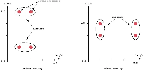
An important component of a clustering algorithm is the distance measure between data points. If the components of the data instance vectors are all in the same physical units then it is possible that the simple Euclidean distance metric is sufficient to successfully group similar data instances. However, even in this case the Euclidean distance can sometimes be misleading. Figure shown below illustrates this with an example of the width and height measurements of an object. Despite both measurements being taken in the same physical units, an informed decision has to be made as to the relative scaling. As the figure shows, different scalings can lead to different clusterings.
Figure 3.5: clustering
Notice however that this is not only a graphic issue: the problem arises from the mathematical formula used to combine the distances between the single components of the data feature vectors into a unique distance measure that can be used for clustering purposes:
K-Mean clustering:
K-means (MacQueen, 1967) is one of the simplest unsupervised learning algorithms that solve the well known clustering problem. The procedure follows a simple and easy way to classify a given data set through a certain number of clusters (assume k clusters) fixed a priori. The main idea is to define k centroids, one for each cluster. These centroids should be placed in a cunning way because of different location causes different result. So, the better choice is to place them as much as possible far away from each other. The next step is to take each point belonging to a given data set and associate it to the nearest centroid. When no point is pending, the first step is completed and an early groupage is done. At this point we need to re-calculate k new centroids as barycenters of the clusters resulting from the previous step. After we have these k new centroids, a new binding has to be done between the same data set points and the nearest new centroid. A loop has been generated. As a result of this loop we may notice that the k centroids change their location step by step until no more changes are done. Finally, this algorithm aims at minimizing an objective function, in this case a squared error function. The objective function
,
where is a chosen distance measure between a data point and the cluster cen tre , is an indicator of the distance of the n data points from their respective cluster centres.
The algorithm is composed of the following steps:
1. Place K points into the space represented by the objects that are being clustered. These points represent initial group centroids.
2. Assign each object to the group that has the closest centroid.
3. When all objects have been assigned, recalculate the positions of the K centroids.
4. Repeat Steps 2 and 3 until the centroids no longer move. This produces a separation of the objects into groups from which the metric to be minimized can be calculated.
centres. The k-means algorithm can be run multiple times to reduce this effect.
K-means is a simple algorithm that has been adapted to many problem domains. As we are going to see, it is a good candidate for extension to work with fuzzy feature vectors.
An example
Suppose that we have n sample feature vectors x1, x2,
..., xn all from the same class, and we know that they fall into
k compact clusters, k < n. Let mi be the mean of the vectors
in cluster i. If the clusters are well separated, we can use a minimum-distance classifier to separate them. That is, we can say that x is in cluster i if || x -mi || is the minimum of all
the k distances. This suggests the following procedure for finding the k means:
Make initial guesses for the means m1, m2, ..., mk
Until there are no changes in any mean
o Use the estimated means to classify the samples into clusters
o For i from 1 to k
Replace mi with the mean of all
of the samples for cluster i
o end_for end_until
Here is an example showing how the
means m1 and m2 move into the centers of two clusters.
Remarks
This is a simple version of the k-means procedure. It can be viewed as a greedy algorithm for partitioning the n samples into k clusters so as to minimize the sum of the squared distances to the cluster centers. It does have some weaknesses:
The way to initialize the means was not specified. One popular way to start is to randomly choose k of the samples.
The results produced depend on the initial values for the means, and it frequently happens that suboptimal partitions are found. The standard solution is to try a number of different starting points.
It can happen that the set of samples closest to mi is
empty, so that mi cannot be updated. This is an
annoyance that must be handled in an implementation, but that we shall ignore. The results depend on the metric used to measure
|| x - mi ||. A popular solution is to normalize each
variable by its standard deviation, though this is not always desirable.
The results depend on the value of k.
This last problem is particularly troublesome, since we often have no way of knowing how many clusters exist.
Unfortunately there is no general theoretical solution to find the optimal number of clusters for any given data set. A simple approach is to compare the results of multiple runs with different k classes and choose the best one according to a given criterion (for instance the Schwarz Criterion but we need to be careful because increasing k results in smaller error function values by definition, but also an increasing risk of overfitting.
IV. RESULT & FUTURE WORK
Magnetic resonance (MR) images are a very useful tool to detect the tumor growth in brain but precise brain image segmentation is a difficult and time consuming process. Manual segmentation of brain tumors from MR images is a challenging and time consuming task.
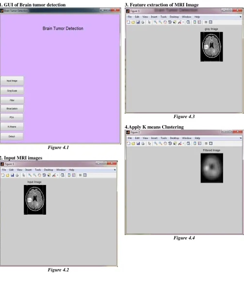
1. GUI of Brain tumor detection
Figure 4.1 2. Input MRI images
Figure 4.2
3. Feature extraction of MRI Image
Figure 4.3 4.Apply K means Clustering
1. Select Region of Interest
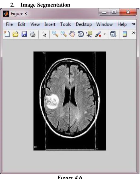
Figure 4.5 2. Image Segmentation
Figure 4.6
3. Detect Brain tumor
Figure 4.7
Future work- A novel algorithm for the segmentation and classification brain tumors is described in this research work. Results and analysis show that the proposed approach is a valuable diagnosing technique. But, in final segmentation, a few other tissues also segmented in addition to tumors. Therefore, in order to improve the accuracy in the segmentation, it is necessary to include additional knowledge for discarding other tissues. In future work, it would be interesting to include additional feature information. Besides the energy, correlation, contrast and homogeneity add more information to the feature extraction in order to make the system more sensitive; information from the textures or location. It will be interesting to continue developing more adaptive models for other types of brain tumors following the same line of work presented here. Another future line would be the detection of small malignant brain tumors. It should be clear that many factors influence the appearance of tumors on images, and although there are some common features of malignancies, there is also a great deal of variation that depends on the tissue and the tumor type. Characteristic features are more likely to be found in large tumors.
V. CONCLUSION