Microsoft
Excel 2013 Plain & Simple
Sebastopol, California 95472
Copyright © 2013 by Curtis D. Frye
All rights reserved. No part of the contents of this book may be reproduced or transmitted in any form or by any means without the written permission of the publisher.
ISBN: 978-0-7356-7243-7
1 2 3 4 5 6 7 8 9 QG 8 7 6 5 4 3
Printed and bound in the United States of America.
Microsoft Press books are available through booksellers and distributors worldwide. If you need support related to this book, email Microsoft Press Book Support at [email protected]. Please tell us what you think of this book at http://www. microsoft.com/learning/booksurvey.
Microsoft and the trademarks listed at http://www.microsoft.com/about/legal/en/us/IntellectualProperty/Trademarks/EN-US. aspx are trademarks of the Microsoft group of companies. All other marks are property of their respective owners.
The example companies, organizations, products, domain names, email addresses, logos, people, places, and events depicted herein are fictitious. No association with any real company, organization, product, domain name, email address, logo, person, place, or event is intended or should be inferred.
This book expresses the author’s views and opinions. The information contained in this book is provided without any express, statutory, or implied warranties. Neither the authors, O’Reilly Media, Inc., Microsoft Corporation, nor its resellers, or distributors will be held liable for any damages caused or alleged to be caused either directly or indirectly by this book.
Acquisitions and Developmental Editor: Kenyon Brown Production Editor: Melanie Yarbrough
Editorial Production: Blue Boot Design Studio Copyeditor: Box Twelve Communications Technical Reviewer: Andy Pope
Contents v
Contents
1
About this book . . . . 1No computerese! . . . .2
Useful tasks… . . . .2
…And the easiest way to do them . . . .2
A quick overview . . . .2
A few assumptions . . . .5
Adapting task procedures for touchscreens . . . .5
A final word (or two) . . . .6
2
What’s new and improved in Excel 2013 . . . . 7Using Excel 2013 in Windows 8 . . . .8
Analyzing data instantly by using the Quick Analysis tool . . . .9
Entering data quickly by using Flash Fill . . . .10
Creating the right chart by using chart recommendations . . . .11
Filtering Excel tables by using slicers . . . .12
Creating a recommended PivotTable . . . .14
Editing a workbook in SkyDrive and the Excel Web App . . . .15
vi Contents
3
Surveying the Excel program window . . . .18Starting Excel . . . .20
Adding Excel 2013 to the Start screen . . . .22
Starting Excel 2013 in Windows 7 . . . .23
Opening existing workbooks . . . .24
Using file properties . . . .26
Creating a new workbook . . . .28
Working with multiple workbooks . . . .29
Sizing and viewing windows . . . .30
Zooming in or out on a worksheet . . . .31
Saving Excel workbooks . . . .32
Changing the default file folder . . . .34
Closing workbooks and exiting Excel . . . .35
Using the Excel Help system . . . .36
Finding Excel Help on the web . . . .37
Searching for a workbook . . . .38
4
Building a workbook . . . . 39Selecting cells . . . .40
Entering text in cells . . . .42
Entering numbers in cells . . . .43
Entering dates and times in cells . . . 44
Entering data using fills . . . .46
Contents vii
Entering data with other shortcuts . . . .50
Creating an Excel table . . . .52
Editing an Excel Table . . . .54
Editing cell contents . . . .56
Inserting a symbol in a cell . . . .57
Creating hyperlinks . . . .58
Creating hyperlinks to web and email resources . . . .60
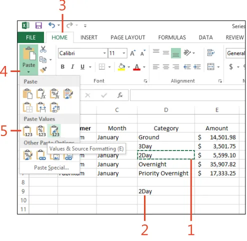
Cutting, copying, and pasting cell values . . . .62
Undoing or redoing an action . . . .63
Pasting values with more control . . . 64
Clearing cell contents . . . .66
Using the Office Clipboard . . . .68
Finding and replacing text . . . .70
Checking the spelling in your worksheet . . . .72
5
Managing and viewing worksheets . . . . 73Viewing and selecting worksheets . . . .74
Renaming worksheets . . . .75
Moving worksheets . . . .76
Copying worksheets . . . .77
Inserting and deleting worksheets . . . .78
Hiding or showing a worksheet . . . .80
Changing worksheet tab colors . . . .81
Inserting, moving, and deleting cells . . . .82
viii Contents
Moving rows or columns . . . .87
Hiding and unhiding columns and rows . . . .88
Entering data and formatting on many worksheets at the same time . . . .90
Changing how you look at Excel workbooks . . . .92
Naming and using worksheet views . . . .94
6
Using formulas and functions . . . . 97Creating simple cell formulas . . . .98
Assigning names to groups of cells . . . 100
Using names in formulas . . . .102
Creating a formula that references values in an Excel table . . . .103
Creating formulas that reference cells in other workbooks . . . 104
Changing links to different workbooks . . . 106
Analyzing data by using the Quick Analysis lens. . . .107
Summing a group of cells without using a formula . . . 108
Creating a summary formula . . . 109
Summing with subtotals and grand totals . . . .110
Exploring the Excel function library . . . 112
Using the IF function . . . .114
Checking formula references . . . .115
Contents ix
7
Formatting the cell . . . . 121Formatting cell contents . . . 122
Formatting part of a cell’s contents . . . .124
Formatting cells containing dates . . . 125
Formatting cells containing numbers . . . 126
Adding cell backgrounds and shading . . . 128
Formatting cell borders . . . 130
Defining cell styles . . . 132
Modifying and deleting cell styles . . . 134
Aligning and orienting cell contents . . . 136
Formatting a cell based on conditions . . . 138
Editing and deleting conditional formats . . . 140
Changing how conditional formatting rules are applied . . . .142
Displaying data bar and icon set formats . . . 144
Displaying color scales based on cell values . . . 146
Deleting conditional formats . . . .147
Merging or splitting cells or data . . . 148
Copying formats with Format Painter . . . 150
8
Formatting the worksheet . . . . 151Applying workbook themes . . . .152
Changing theme fonts and effects . . . 154
Creating new workbook themes . . . 156
Coloring sheet tabs . . . .157
x Contents
Inserting rows or columns . . . .162
Setting insert options . . . .163
Moving rows and columns . . . 164
Deleting rows and columns . . . 166
Grouping and ungrouping worksheet rows . . . .167
Hiding rows and columns . . . 168
Outlining to hide and show rows and columns . . . .170
Protecting worksheets from changes . . . .171
Locking cells to prevent changes . . . .172
9
Printing worksheets . . . . 173Previewing worksheets before printing . . . .174
Printing worksheets with current options . . . .176
Choosing whether to print gridlines and headings . . . .177
Choosing printers and paper options . . . .178
Printing part of a worksheet . . . 180
Printing row and column headings on each page . . . .181
Setting and changing print margins . . . 182
Setting page orientation and scale . . . 184
Creating headers and footers . . . 186
Adding graphics to a header or a footer . . . 188
Contents xi
10
Customizing Excel to the way you work . . . . 193Opening ready-to-use workbook templates . . . 194
Saving a workbook as a template . . . 196
Adding commands to the Quick Access toolbar . . . 198
Moving the Quick Access toolbar . . . 200
Removing a ribbon element . . . 201
Adding and reordering ribbon elements . . . 202
Creating new ribbon tabs and groups . . . 204
Renaming a ribbon element . . . 206
Choosing the color Excel uses to display errors . . . 207
Hiding and displaying ribbon tabs . . . 208
Controlling which error messages appear . . . .210
Defining AutoCorrect entries . . . 212
Controlling AutoFormat rules . . . .214
11
Sorting and filtering worksheet data . . . . 215Sorting worksheet data . . . .216
Creating a custom sort list . . . .218
Filtering data quickly with AutoFilter . . . 220
Filtering data with a search filter . . . 222
Clearing a filter . . . .224
Creating an advanced filter . . . 226
xii Contents
Validating data using a list . . . 234
Creating a recommended PivotTable . . . 236
12
Summarizing data visually using charts . . . . 239Creating a chart . . . 240
Changing a chart’s layout and style . . . .242
Changing a chart’s appearance . . . 244
Formatting chart legends and titles . . . 246
Adding and removing data labels and grid lines . . . 248
Formatting chart axes . . . 250
Changing a chart’s data source . . . .252
Adding and deleting data series . . . 254
Filtering charts . . . .256
Manipulating pie charts . . . 258
Creating a stock chart . . . 260
Adding a trendline to a chart . . . .261
Summarizing data using sparklines . . . 262
Contents xiii
13
Enhancing your worksheets with graphics . . . . 267Adding drawing objects to a worksheet . . . .269
Adding graphics to worksheets . . . .270
Adding text to a shape . . . 272
Applying shape styles . . . 273
Changing a shape’s fill color or image . . . .274
Adding effects to drawing objects . . . .276
Resizing and rotating pictures and objects . . . .278
Removing the background from an image . . . 280
Aligning and grouping drawing objects . . . 282
Using WordArt to create text effects in Excel . . . 284
Inserting clip art into a worksheet . . . 286
Inserting and changing a diagram . . . 288
Creating an organization chart . . . 290
Changing the layout and design of a SmartArt graphic . . . 292
Adding an equation to a shape . . . 294
Reordering objects . . . 296
14
Sharing Excel data with other programs . . . . 297Linking and embedding other files . . . 300
Exchanging table data between Excel and Word . . . 302
Copying Excel charts and data into PowerPoint . . . 304
Exchanging data between Access and Excel . . . 306
xiv Contents
15
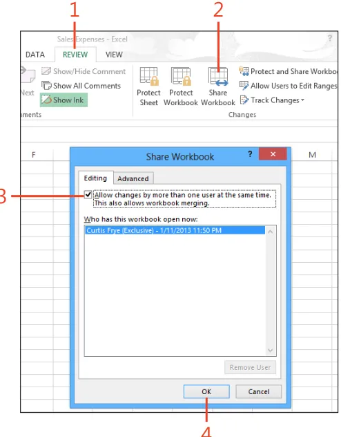
Sharing workbooks in Excel . . . .312Adding and viewing cell comments . . . .313
Editing and deleting comments . . . .314
Tracking changes in workbooks . . . .315
Accepting or rejecting changes . . . .316
Maintaining a change history . . . .318
Saving worksheets to the web . . . 320
Dynamically updating worksheets published to the web . . . 322
Retrieving web data using Excel . . . .324
Copying web data to Excel . . . .326
Modifying web queries . . . 327
Saving data to the cloud using SkyDrive . . . 329
Interacting over the web using XML . . . 330
Editing a workbook in the Excel Web App . . . .332
Sharing Excel workbooks on the web . . . 334
Making workbooks available on the web . . . 336
In this section:
■
■ No computerese!
■
■ A quick overview
■
■ A few assumptions
■
■ Adapting task procedures for touchscreens
■
■ A final word (or two)
About this book
1
No computerese!
Let’s face it—when there’s a task that you don’t know how to do but you need to get it done in a hurry, or when you’re stuck in the middle of a task and can’t figure out what to do next, there’s nothing more frustrating than having to read page after page of technical background material. You want the informa-tion you need—nothing more, nothing less—and you want it now! It should be easy to find and understand.
That’s what this book is all about. It’s written in plain lan-guage—no jargon. There’s no single task in the book that takes more than a couple pages. Just look up the task in the index or the table of contents, turn to the page, and there’s the informa-tion you need, laid out in an illustrated, step-by-step format. You don’t get bogged down by the whys and wherefores: just follow the steps, and get your work done.
Occasionally, you might have to turn to another page if the pro-cedure you’re working on is accompanied by a See Also refer-ence. That’s because a lot of tasks overlap, and I didn’t want to keep repeating myself. I’ve scattered some useful tips here and there, and I’ve thrown in a Try This or a Caution occasionally, but by and large, I’ve tried to remain true to the heart and soul of a Plain & Simple book, which is that the information you need should be available to you at a glance.
Useful tasks…
Whether you use Excel 2013 at home or on the road, I’ve tried to pack this book with procedures for everything I could think of that you might want to do, from the simplest tasks to some of the more esoteric ones.
…And the easiest way to do them
Another thing I’ve tried to do in this book is to find and docu-ment the easiest way to accomplish a task. Excel 2013 often provides a multitude of methods to accomplish a single end result—which can be daunting or delightful, depending on the way you like to work. If you tend to stick with one favorite and familiar approach, I think the methods described in this book are the way to go. If you like trying out alternative techniques, go ahead! The intuitiveness of Excel 2013 invites exploration, and you’re likely to discover ways of doing things that you think are easier or that you like better than mine. If you do, great! It’s exactly what the developers of Excel 2013 had in mind when they provided so many alternatives.
A quick overview
Your computer probably came with Excel 2013 preinstalled, but if you do have to install it yourself, setup makes installation so simple that you won’t need my help anyway. So, unlike many computer books, this one doesn’t start with installation instruc-tions and a list of system requirements.
Next, you don’t have to read the sections of this book in any particular order. You can jump in, get the information you need, and then close the book and keep it near your computer until the next time you need to know how to get something done. But that doesn’t mean I scattered the information about with wild abandon. I’ve organized the book so that the tasks you want to accomplish are arranged in two levels—you find the general type of task you’re looking for under a main section title, such as “Formatting the worksheet,” “Summarizing data visually using charts,” “Using Excel in a group environment,” and so on. Then, in each of those sections, the smaller tasks within
the main task are arranged in a loose progression from the sim-plest to the more complex.
Section 1 (this section) introduces the book, while Section 2, “What’s new and improved in Excel 2013,” fills you in on the most important new features of Excel 2013, which include the program’s seamless integration with Microsoft Windows 8. Excel 2013 also gives you new ways to analyze your data quickly, whether using the Quick Analysis tool, Recommended Charts, Recommended PivotTables, and editing and sharing your data on the web by using SkyDrive and Excel Web App.
Section 3, “Getting started with Excel 2013,” and Section 4, “Building a workbook,” cover the basics: starting Excel 2013 and shutting it down, sizing and arranging program windows, navigating in a workbook, using the user interface ribbon to have Excel do what you want it to do, and working with multiple Excel documents at the same time. Section 3 also introduces galleries, which are collections of preset formats that you can apply to worksheets, charts, and other Excel objects, and shows you how to get help from within Excel and on the web. Section 4 contains a lot of useful information about entering text and data, including shortcuts you can use to enter an entire series of numbers or dates by typing values in just one or two cells. You’ll also learn about using the Office Clipboard to manage items that you cut and paste, running the spelling checker to ensure
that you haven’t made any errors in your workbook, and finding and replacing text to update changes in information, such as customer addresses or product names.
Section 5, “Managing and viewing worksheets,” is all about using worksheets—the “pages” of a workbook. In this section, you’ll find out about selecting, renaming, moving, copying, inserting, and deleting worksheets, rows, columns, and cells. In Section 6, “Using formulas and functions,” you’ll get to know formulas and functions. You use formulas to calculate values, such as finding the sum of the values in a group of cells. After you’re up to speed on creating basic formulas, you’ll learn how to save time by copying a formula from one cell and pasting it into as many other cells as you like. Finally, you’ll extend your knowledge of formulas by creating powerful statements using the function library in Excel 2013.
Section 7, “Formatting the cell,” focuses on making your work-books’ cells look great. Here’s where you’ll learn techniques to make your data more readable, such as by changing font sizes and font colors and by adding colors and shading to cells. Section 8, “Formatting the worksheet,” describes similar techniques you can apply to your worksheets, such as moving,
you need to see all of the sales for a specific product but don’t want to bother with the rest of the data for the moment? No problem.
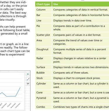
A picture is worth ten thousand words (according to Confucius; the modern version of the saying shorts you by nine thou-sand words), and in Section 12, “Summarizing data visually using charts,” I’ll show you how to use the Excel 2013 charting engine to create and use charts—including sparkline charts—to inserting, and deleting rows and columns, applying worksheet
themes, and coloring sheet tabs to call attention to important information.
Section 9, “Printing worksheets,” is all about printing your Excel documents, whether that means printing all or just a portion of your results. Your productivity should increase after reading Section 10, “Customizing Excel to the way you work,” where I’ll show you how to add commands to the Quick Access toolbar, customize the tabs on the ribbon user interface, control which error messages appear, define rules that Excel uses to replace often-misspelled words, create workbooks from built-in tem-plates, and create custom workbook templates that you can use to create new workbooks based on those formats.
Section 11, “Sorting and filtering worksheet data,” provides you with techniques that you can use to limit the data displayed in a worksheet and determine the order in which it is presented. Do
summarize your data visually. In Section 13, “Enhancing your worksheets with graphics,” you’ll learn just how easy it is to insert clip art, add a special text effect, or resize a photo that you added to a worksheet.
Section 14, “Sharing Excel data with other programs,” and Sec-tion 15, “Using Excel in a group environment,” are all about sharing the data in your Excel worksheets—whether it’s with your colleagues, on the Internet, or with other programs. Sec-tion 14 shows you how to make Excel 2013 interact with other Microsoft Office 2013 programs, such as by embedding docu-ments from other programs in your Excel workbooks, exchang-ing data between Excel and Word, or importexchang-ing a text file into an Excel worksheet. In Section 15, you’ll learn how to use Excel
A few assumptions
I had to make a few educated guesses about you, my audience, when I started writing this book. Perhaps you just use Excel for personal reasons, tracking your household budget, doing some financial planning, or recording your times for weekend bike races. Maybe you run a small, home-based business, or you’re an employee of a corporation where you use Excel to analyze and present sales or production data. Taking all these possi-bilities into account, I assumed that you need to know how to create and work with Excel workbooks and worksheets, sum-marize your data in a variety of ways, format your documents so that they’re easy to read, and then print the results or share them over the web or distribute your data both ways.
Another assumption I made is that—initially, anyway—you use Excel 2013 just as it came, meaning that you’d be working with the standard user interface. I’ve written the procedures and captured the graphics throughout this book based on the Excel 2013 user interface as it was installed on my computer.
Adapting task procedures for
touchscreens
In this book, we provide instructions based on traditional keyboard and mouse input methods. If you’re using Excel on a touch-enabled device, you might be giving commands by tap-ping with your finger or with a stylus. If so, substitute a taptap-ping action any time we instruct you to click a user interface element. Also note that when we tell you to enter information in Excel, you can do so by typing on a keyboard, tapping in the entry field under discussion to display, and using the onscreen key-board, or even speaking aloud, depending on your computer setup and your personal preferences.
in a group environment, to add comments to your worksheets, and to accept or reject the comments made by others. You’ll also learn how to publish a worksheet to the web as well as how to pull information from the Internet directly into your worksheets and to share and edit your workbooks using Excel Web App. This section also introduces XML (an abbreviation for Extensible Markup Language), a handy technology that enables you to exchange data between spreadsheet applications.
A final word (or two)
I had three goals in writing this book:
1 Whatever you want to do, I want the book to help you get it done. 2 I want the book to help you discover how to do things you didn’t
know you wanted to do.
3 And, finally, if I’ve achieved my first two goals, I’ll be well on the way to the third, which is for my book to help you enjoy using Excel 2013. I think that’s the best gift I could give you to thank you for buying my book.
I hope you’ll have as much fun using Microsoft Excel 2013 Plain
& Simple as I’ve had writing it. The best way to learn is by doing,
and that’s how I hope you’ll use this book.
Jump right in!
T
his section of the book introduces a selection of the new and improved features in Excel 2013: using Excel 2013 in Windows 8, analyzing data by using the Quick Analysis tool, entering data quickly by using Flash Fill, creating recommended charts, formatting charts by using the new format-ting tools, filtering Excel tables by using slicers, creaformat-ting a recommended PivotTable, and editing a workbook in SkyDrive and the Excel Web App.In this section:
■
■ Using Excel 2013 in Windows 8
■
■ Analyzing data instantly by using the
Quick Analysis tool
■
■ Entering data quickly by using Flash Fill
■
■ Creating the right chart using chart
recommendations
■
■ Formatting charts by using the new
tools interface
■
■ Filtering Excel tables using slicers
■
■ Creating a recommended PivotTable
■
■ Editing a workbook in SkyDrive and
Excel Web App
What’s new
and improved in
Launch Excel 2013 in Windows 8
1 If necessary, press Ctrl+Esc to display the Start screen.
2 If necessary, scroll to the Start screen to display the Excel 2013 tile. 3 Click the Excel 2013 tile.
Using Excel 2013 in Windows 8
After you install Excel on your computer, you can start it from the Start screen in Windows 8, which opens the program with a new, blank workbook. You can also start Excel in Windows 8
by pinning it to the taskbar and clicking it when viewing your computer in Desktop mode.
3
2
Summarize data by using Quick Analysis
1 Select the cell range that you want to summarize.
2 Click the Quick Analysis action button to display the Quick Analysis tools available to you.
3 Click the label representing the category of tools that you want to use.
4 Click the button representing the summary that you want to create.
Analyzing data instantly by using the Quick Analysis tool
One of the refinements in Excel 2013 is the Quick Analysis Lens, which brings the most commonly used formatting, charting, and summary tools into one convenient location. You have a wide range of tools available to you, including the ability to create an Excel table or PivotTable, insert a chart, or add conditional
formatting. You can also add total columns and rows to your data range. For example, you can click Totals and then Running Total for columns, identified by the icon labeled Running Total and the yellow column at the right edge of the button, to add a column that calculates the running total for each row.
4
1
2 3
TIP You can add one summary column and one summary row to each data range. If you select a new summary column or row when one exists, Excel displays a confirmation dialog box to verify that you want to replace the existing summary. When you click yes, Excel makes the change.
Separate data by using Flash Fill
1 Click the cell to the right of the first row that you want to work with. 2 Type the value that you want to extract from the row, and press
Enter.
3 In the cell directly below the first, start typing the extracted value for the row.
4 Press Enter to accept the suggested Flash Fill values for the remain-ing rows.
5 If desired, repeat the process in the cell to the right of the first cell in the new column to extract another value from the row’s original data.
Entering data quickly by using Flash Fill
Your data sets might contain values in a single cell that you’d like to divide into separate cells. For example, your worksheet might contain a list of names where the first name, middle initial, and last name all appear in the same cell. If you need to separate the first name, middle initial, and last name into sepa-rate cells, you can do so by using Flash Fill, which is new in Excel 2013.
To use Flash Fill, click a cell to the right of the list that contains the data that you want to work with, and then type the correct
value for that cell. For example, your list might contain the name Mark Hassall. If you want to store the person’s first name in one cell and last name in another, you would type Mark in the first cell and hassall in the second. You then repeat the process for the second row of the list, at which point Flash Fill recognizes the data pattern and offers to fill in the remaining values.
If your data set contains rows with additional data, such as a middle initial, you can correct the first example of that differing pattern to update similar rows in the new columns.
4 3
1
2
5
Create a recommended chart
1 Click a cell in the data list that you want to summarize. 2 Click the Insert tab.
3 Click Recommended Charts.
4 Click the chart that you want to create. 5 Click OK.
Creating the right chart by using chart recommendations
You can create a chart manually, or you can create a chart that the program recommends. The Recommended Charts gallery, which is new in Excel 2013, displays a set of charts that you can
create based on your data. All you need to do is click the chart that you want and confirm your choice. In either case, you can then change a chart’s appearance with no trouble at all.
1 2
3
5
4
Add a slicer
1 Click any cell in the Excel table that you want to filter. 2 Click the Insert tab.
3 Click Slicer.
4 Select the check box next to each column by which you want to filter the table.
5 Click OK.
Filtering Excel tables by using slicers
In versions of Excel prior to Excel 2013, the only visual indication that you had applied a filter to an Excel table column was the indicator added to the column’s filter arrow. The indicator told users that there was an active filter applied to that column but
provided no information about which values were displayed and which were hidden. In Excel 2013, slicers provide a visual indica-tion of which items are currently displayed or hidden in an Excel table field.
1
4
5
2
3
Define a filter by using a slicer
1 In the slicer, do any of the following:
a Click an item to display just its related values.
b While pressing the Ctrl key, select multiple items to display those items’ related values.
c While pressing the Shift key, click two items to display related values for every value from the first selected item to the second selected item in the slicer’s list.
1
Create a recommended PivotTable
1 Click any cell in the Excel table or data list that you want to summarize.
2 Click the Insert tab.
3 Click Recommended PivotTables.
4 Click the PivotTable that you want to create. 5 Click OK.
Creating a recommended PivotTable
Excel workbooks enable you to store and summarize large data collections effectively. As versatile as Excel tables and formu-las are, they are static. After you create a data arrangement or summary in a standard worksheet, you can change it only by copying, pasting, or moving your data and altering your
formulas. You can extend those capabilities by creating Pivot-Tables. PivotTables are powerful and versatile tools that let you rearrange, sort, and filter your data dynamically, without editing your data or changing any formulas.
4
5
1 3 2
Edit a file in the Excel Web App
1 In your web browser, navigate to http://www.skydrive.com. 2 Navigate to the folder that contains the file that you want to edit. 3 Click the tile of the file that you want to edit.
Editing a workbook in SkyDrive and the Excel Web App
The SkyDrive service and Microsoft Office 365 provide access to the Office Web Apps, which let you create and edit Office documents in your web browser. The Microsoft Excel Web App provides a rich set of capabilities that you can use to create new
workbooks and edit workbooks that you created in the desktop version of the application. If you find that you need some fea-tures that aren’t available in the Excel Web App, you can open the file in the Excel 2013 desktop application.
3
1
2
Formatting charts by using the new tools interface
Charts summarize data visually, so every chart has a particu-lar arrangement and presentation of its elements. The overall arrangement of a chart’s elements is its layout, whereas the overall appearance of the chart’s elements is its style. You can
apply predefined layouts and styles to your charts. As with any formatting that you apply, you can always fine-tune your choices later.
Change a chart’s style
1 Click the chart that you want to change. 2 Click the Chart Styles button.
3 In the Chart Styles gallery that appears, click the new style.
1
2
3
M
icrosoft Excel 2013 is designed to help you store, summarize, and present data relevant to your business or home life. You can create spreadsheets to track products and sales or—just as easily—build spread-sheets to keep track of your personal investments or your kids’ soccer scores. Regardless of the specific use that you have in mind, Excel is a ver-satile program that you can use to store and retrieve data quickly.Working with Excel is pretty straightforward. The program has a number of preconstructed workbooks that you can use for tasks such as tracking work hours for you and your colleagues or computing loan payments, but you also have the freedom to create and format workbooks from scratch, giving you the flexibility to build any workbook that you need.
This section of the book covers the basics: how to start Excel and shut it down, how to open Excel documents, how to change the Excel window’s size and appearance, and how to get help from within the program. There’s also an illustrated overview of the Excel window, with labels for the most important parts of the program, and a close-up look at the new user interface. You can use the images in this section as touchstones for learn-ing more about Excel.
In this section:
■
■ Surveying the Excel program window ■
■ Starting Excel in Windows 8 ■
■ Adding Excel 2013 to the Start screen ■
■ Starting Excel 2013 in Windows 7 ■
■ Opening, searching for, and assigning
properties to workbooks
■
■ Creating a new workbook ■
■ Working with multiple workbooks ■
■ Sizing, viewing, and zooming windows ■
■ Saving Excel workbooks ■
■ Closing workbooks and exiting Excel ■
■ Using the Excel Help system
Getting started
Working with the user interface
Excel 2013 incorporates the ribbon user interface. In Excel 2013, you can find what you need in one place: the ribbon at the top of the screen.
Surveying the Excel program window
In many ways, an Excel worksheet is like the ledger in your checkbook. The page is divided into rows and columns, and you can organize your data by using these natural divisions as a guide. The box formed by the intersection of a row and a column is called a cell. You can identify an individual cell by its
column letter and row number. This combination, which identi-fies the first cell in the first column as cell A1, is called a cell ref-erence. The following graphic shows you the important features of the Excel 2013 screen.
All button
Row heading File tab
Ribbon tab
Sheet tabNew sheet button Status bar Horizontal scrollbar Formula bar
Title bar Column headingVertical scrollbar Active cell
Working with galleries
After you enter your data in a worksheet, you can change the appearance of data and objects within the worksheet by using galleries that appear on the user interface. The ribbon has three types of galleries: galleries that appear in a dialog box, galleries that appear as a drop-down menu when you click a user inter-face item, and galleries that appear within the user interinter-face itself. The following graphic shows a styles gallery.
Excel 2013 lets you see how formatting will appear before you apply a formatting change. Rather than make you apply the change and then remove it if you don’t like how it turned out, when you hover your mouse pointer over a style in a gallery, Excel 2013 generates a live preview of how your data or object will appear if you apply that style. All you need to do is move your mouse to see what your objects will look like when you’re finished.
TIP If positioning your mouse pointer over an icon in a gallery doesn’t result in a live preview, that option might be turned off in your copy of Excel 2013. To turn Live Preview on, click the File tab, and then click Options to display the Excel Options dialog box. Click General, select the Enable Live Preview check box, and click OK.
Start Excel 2013 in Windows 8
1 If necessary, press Ctrl+Esc to display the Start screen.
2 If necessary, scroll to the Start screen to display the Excel 2013 tile. 3 Click or tap the Excel 2013 tile.
Starting Excel
After you install Excel on your computer, you can start it from the Start page in Windows 8, which opens the program with a new, blank workbook. You can also start Excel in Windows 8
by pinning it to the taskbar and clicking it when viewing your computer in Desktop mode.
3
2
Pin Excel 2013 to the taskbar
1 If necessary, press Ctrl+Esc to display the Start screen.
2 If necessary, scroll to the Start screen to display the Excel 2013 tile. 3 Right-click the Excel 2013 tile.
4 Click Pin To Taskbar.
4
3
2
TIP To hide the action bar at the bottom of the screen without making any changes, press Esc.
Add Excel 2013 to the Start screen
1 Open File Explorer.
2 Navigate to the folder that contains the Excel.exe program file. 3 Right-click the Excel.exe file.
4 Click Pin to Start.
Adding Excel 2013 to the Start screen
The Windows 8 Start screen provides a solid base of opera-tions for your work in Excel. Running a program from the Start screen is as easy as clicking or tapping its tile. If for some reason
Excel 2013 doesn’t appear on your Start screen, you can add it quickly.
3 2
4
Start Excel 2013 in Windows 7
1 Click the Start button on the taskbar. 2 Click All Programs.
3 Click Microsoft Office 2013. 4 Click Excel 2013.
Starting Excel 2013 in Windows 7
If your computer uses the Microsoft Windows 7 operating system, you can run Excel 2013 by opening the Start menu, displaying the Microsoft Office 2013 programs, and clicking
Excel 2013. You can display the Start menu by clicking the Start button or by pressing Ctrl+Esc, whichever is faster for you.
1
2
3
4
open a workbook
1 Click the File tab. 2 Click Open. 3 Click Computer. 4 Click Browse.
opening existing workbooks
After you create an Excel workbook, you will probably want to open it again, whether to verify the contents, add or update data, or copy data from one workbook to another. If you know where in your file system your workbook is stored, you can use
the Open dialog box within Excel to locate and open your file. If you worked with your file recently, you can probably also find it in the Recent Workbooks list in the Backstage view that you display by clicking the File tab.
4
2
3
(continued on next page)
5 Navigate to the folder that contains the workbook that you want to open.
6 Click the workbook. 7 Click Open.
open a workbook
(continued)2
3
4
TIP You can also display the Open page of the Backstage view by pressing Ctrl+O.
open a recently used workbook
1 Click the File tab. 2 Click Open.
3 Click Recent Workbooks.
4 Click the workbook that you want to open.
5
6
7
Set file properties
1 Open the file to which you want to assign property values. 2 Click the File tab.
3 Click Info. 4 Click Properties.
5 Click Show Document Panel. 6 Add information describing your file.
Using file properties
Finding files can be difficult on computers that you share with your colleagues or if you’ve been using the same computer for a long time and have created a lot of workbooks. You can make it easier to find your files by adding descriptive terms to their
Properties fields. If you enter a term in a Properties field, you can search using that term, even if it doesn’t occur within the body of the workbook.
4 5
3
6
TIP Adding words to the Keywords field is a great way to improve search results. Just type a word, press the Spacebar, and then type the next word. There’s no need to use commas.
Define custom properties
1 Open the file to which you want to assign property values. 2 Click the File tab.
3 If necessary, click Info. 4 Click Properties.
5 Click Advanced Properties. 6 Click the Custom tab.
7 Type the name of the custom property.
8 Select the type of data contained in the property. 9 Type a value for the property.
10 Click Add. 11 Click OK.
4 5
3
11
7
6 10
8
9
TRY ThIS Excel comes with a set of predefined custom properties, such as Checked By and Date Completed. To use an existing custom property, display the Custom tab of the Properties dialog box, click the name of the custom property, type a value for the property in the Value box, and click OK.
Create a new workbook
1 Click the File tab. 2 Click New.
3 Click Blank Workbook.
Creating a new workbook
As a general rule, you should create a new workbook any time that you need a place to store data on a new subject. For exam-ple, you might track your company’s sales in one workbook, the
products your company offers in another, and your employees’ personal information and salaries in another.
3
2
TIP You can create a new, blank workbook by pressing Ctrl+N at any time that you are not in Backstage view (which appears when you click the File tab). To exit Backstage view, click the Return To Workbook button.
Switch between open workbooks
1 Click the View tab. 2 Click Switch Windows.
3 Click the name of the workbook that you want to display.
Working with multiple workbooks
When you create an Excel workbook for each subject of your business, you sometimes need to look at data from more than one workbook to make your decisions. In cases like this, you can switch between workbooks by choosing the workbook’s name
from the list displayed when you click the Switch Windows button on the View tab. You can also choose one of several arrangements so that you can work with your workbooks effectively.
Show more than one workbook
1 Click the View tab. 2 Click Arrange All.
3 Select the arrangement that you want. 4 Click OK.
1
2
3
3
4
1 2
Resize a window
1 Click the Maximize button to make the window take up the entire screen.
2 Click the Minimize button to represent the window as a button on the taskbar.
3 Click the Restore button to return the window to its previous size. 4 Drag the left or right border of the window to resize it horizontally. 5 Drag the top or bottom border of the window to resize it vertically. 6 Drag a corner to resize the window both horizontally and vertically. 7 Drag the window’s title bar to change its position.
Sizing and viewing windows
You work with windows in the Excel program the same way you work with windows on your desktop. You can make a work-book’s window as large as the screen itself. If you have more
than one workbook open at a time, you can choose from several display arrangements to order the windows most effectively.
Title Bar Minimize
RestoreResize
TIP The Maximize and Restore buttons are actually two states of the same “window size” button, so you never see them on a window at the same time.
Zoom in or out
1 Click the Zoom In control to make your window’s contents 10 per-cent larger per click.
2 Click the Zoom Out control to make your window’s contents 10 percent smaller per click.
3 Drag the Zoom slider control to the left to zoom out or to the right to zoom in.
Zoom in or out to a custom zoom level
1 Click the View tab. 2 Click Zoom.
3 Select the Custom option.
4 Type a new zoom level in the Custom field. 5 Click OK.
Zooming in or out on a worksheet
If you are not satisfied with how much of your worksheet you can see, you can make the worksheet larger or smaller without changing the window size. When you zoom out on a worksheet,
you can see the overall layout, but it might be difficult to read the data in individual cells. To get a better look at the data in your cells, you can zoom in on your worksheet.
Zoom in Zoom out
Zoom slider
3
5
4
1
2
TIP The maximum zoom level is 400 percent; the minimum zoom level is 10 percent.
Save a workbook
1 Click the Save button on the Quick Access toolbar.
Save a workbook with a new name
1 Click the File tab. 2 Click Save As. 3 Click Computer. 4 Click Browse.
Saving Excel workbooks
There’s nothing more frustrating than losing a few minutes or even hours of work because you forget to save your file. When you close your workbook, Excel checks to see whether it has changed since the last time you saved it. If it has been changed,
you’re asked whether you want to save your workbook before you close it. If you want to save multiple versions of the same workbook, you can create a copy of your file by saving it with a different name.
1
4
2
3
(continued on next page)
5 Navigate to the directory where you want to save your file. 6 Type a new file name.
7 Click Save.
TIP You can also save a workbook by pressing Ctrl+S. A good rule is to save your workbook every time you make a change that you would hate to have to make again.
6
7
5
Save a workbook with a new name
(continued)Change the default file folder
1 Click the File tab. 2 Click Options.
3 Click Save in the Excel Options dialog box.
4 In the Default Local File Location box, type the path for the folder that you want to appear by default.
5 Click OK.
Changing the default file folder
When you display the Open, Save, and Save As dialog boxes in Excel, the program opens to its default folder, which is usually your Documents folder. If you frequently open workbooks that
are saved in folders other than Documents, you can change the folder that Excel displays by default.
2
4
5
3
Close a workbook
1 Click the File tab. 2 Click Close.
3 If a dialog box appears asking whether you want to save any unsaved changes, you can do any of the following:
a Click Save to save the workbook using the same name and location.
b Click Don’t Save to discard all the changes made since the work-book was last saved.
c Click Cancel to return to the workbook.
Closing workbooks and exiting Excel
When you’re done working with an Excel workbook, you can close it to reduce the clutter on your desktop and the amount of memory that your computer uses to manage its programs.
You can also exit the Excel program when you’ve completed your work and are ready to move on to other tasks.
2
1
Exit Excel
1 Click the Close button at the top-right corner of the program window.
Get Microsoft Excel help
1 Click the Microsoft Excel Help button.
Using the Excel help system
If you need to get help for using Excel, you can look in a number of places. One option is to right-click an object (such as a worksheet or a graphic) to see a list of things that you can
do with the object. You can also open the Excel Help files and browse through them to find the answer to a specific question or just to explore.
1
Get suggested commands from shortcut
menus
1 Right-click any Excel object to see the shortcut menu of commands. 2 Click a command.
2
1
Get help on the web
1 Click the Microsoft Office Excel Help button. 2 Type your search terms.
3 Click the Search button.
4 Browse the topics displayed for help and resources.
Finding Excel help on the web
The Excel Help system extends well beyond the files installed
with your program. There are a multitude of helpful resources on the web, which you can search for from within the Excel Help system.
TIP You can visit the Microsoft Office Online site directly by opening your web browser and typing office .microsoft .com/ in the address box. You can find numerous links to help and how-to files on that page.
1
3
4
2
Search for a workbook
1 Press Windows+C to display the charms. 2 Click Search.
3 Click Files.
4 Type a search term.
5 Click the file that you want to open.
Searching for a workbook
When you work in Excel for a while, it’s likely that you’ll create lots of workbooks and save them in many different places. If you don’t know the exact name of the file that you want to
open or its location, but you do know part of its name or some of the data it contains, you can search for the file and open it after you locate it.
3
5
4
2
In this section:
■
■ Understanding how Excel interprets
data entry
■
■ Navigating the worksheet and selecting
cells
■
■ Entering text, numbers, dates, and
times in cells
■
■ Entering data using fills, Flash Fill, and
other shortcuts
■
■ Creating an Excel table
■
■ Editing cell contents and inserting
symbols into a cell
■
■ Creating hyperlinks
■
■ Cutting, copying, pasting, finding, and
replacing cell values
■
■ Undoing or redoing an action
■
■ Checking the spelling in your
worksheet
Building a
workbook
4
Selecting cells
Whenever you make changes to cells in a worksheet, you can save time by applying the changes to similar cells at the same time. In Excel 2013, you can select groups of cells that aren’t
even next to each other. If your worksheet stores dates in cells with other information in cells in between, you can select all the date cells and apply a format to them at the same time.
Select a contiguous group of cells
1 In the group that you want to select, drag from the upper-left cell to the lower-right cell.
Select a noncontiguous group of cells
1 Drag from the upper-left cell you want to select to the lower-right cell to select the first set of cells.
2 Hold down the Ctrl key, and drag to select another set of cells.
1
1
2
Select rows or columns
1 Click the header for the first row or column you want to select. 2 Hold down the Shift key, and click the header for the last row or
column you want to select.
Select noncontiguous rows or columns
1 Click the header of the first row or column you want to select, hold down the Ctrl key, and click the headers of the other rows or columns.
TIP To cancel the selection of a group of cells, rows, or columns, click any cell in the worksheet.
1
1
2
Column headerEnter text with forced line breaks
1 Click the cell in which you want to enter text.
2 Type the text that you want to appear on the first line. Press Alt+Enter to insert a line break.
3 Type the text that you want to appear on the second line, and then press Enter.
Enter text as one line
1 Click the cell in which you want to enter text. 2 Type the text that you want to appear. 3 Press Enter.
Entering text in cells
No workbook worthy of the name stays empty for long. You can type any sort of text you want directly in a cell, whether the text is a label identifying the data in a row or column or an expla-nation reminding you and your colleagues of any limitations
on the data to be entered in a cell. Most text entered in Excel workbooks is short enough to fit on one line, but if you want to have the text in a cell appear on two or more lines and break at a specific location, you can easily insert a line break.
SEE ALSo For information about how to make your columns wider to allow more text to appear within a cell, see “Resize a column” on page 160.
TIP In Excel 2013, the formula bar doesn’t automatically expand to display all the information in a cell. To scroll through the contents of the formula bar one line at a time, use the scroll buttons at the right edge of the formula bar. To display the formula bar’s entire contents, click the Expand Formula Bar control to the right of the formula bar. When you expand the formula bar, the Expand Formula Bar control changes to the Collapse Formula Bar control; clicking it returns the formula bar to its original one-line height.
2
1
3
1
2
Enter numbers
1 Click the cell in which you want to enter a number. 2 Type a numerical value.
3 Press Enter.
Entering numbers in cells
The backbone of any workbook is the numerical data in its worksheets, whether that data reflects sales, employee salaries, or the quantity of a given product that you have in inventory. Entering numbers in Excel is as simple as clicking the cell and typing, but you can also enter very large or very small numbers using scientific notation. In scientific notation, a number with
a positive exponent is written as 1.00E+06, which is read as “one times ten to the sixth power.” Numbers that are less than one can be written with negative exponents. For example, the number .001 would be written as 1.00E-03 and read as “one times ten to the negative third power.”
Enter numbers using scientific notation
and exponents
1 Click the cell in which you want to enter a number. 2 Type the base number you want.
3 Type E.
4 Type the exponent you want. 5 Press Enter.
TIP You can type a number but have it interpreted as a text value by typing ‘ (an apostrophe) before the number value. The apostrophe will not appear in the cell, but a green icon will appear in the corner of the cell; clicking the cell exposes formatting options you can apply to the data.
SEE ALSo For information about applying number formatting such as dollar and percent signs instead of typing them, see “Formatting cells containing numbers” on page 126.
1
2
2 3 4
1
Enter a date
1 Click the cell in which you want to enter a date.
2 Type the month, day, and year, with each number separated by a slash (/) or a hyphen (-).
3 Press Enter.
Enter a time
1 Click the cell in which you want to enter a time.
2 Type the hour, a colon (:), and the minutes. Press the spacebar, and type a or p for A.M. or P.M.
3 Press Enter.
Entering dates and times in cells
Dates are extremely important in any business or personal
situ-ation, so Excel takes care to get them right. Excel understands dates no matter how you type them, so feel free to type them as needed. You can always change the formatting later.
CAUTIoN Your regional settings affect which entries Excel interprets as dates. In countries that represent dates using the Day/Month/Year format, 9/25/2013 would be interpreted as a text entry because there are only 12 months in a year.
1
2
1 2
Enter a date and time
1 Click the cell in which you want to enter a date and time. 2 Type a date, press the spacebar, and then type a time. 3 Press Enter.
Enter the current date and time
1 Click the cell in which you want to enter the current date and time. 2 Type =NoW().
3 Press Enter.
TIP You can enter the current date by pressing Ctrl-; and the current time by pressing Ctrl-Shift-;. These values are entered as static values and won’t change when Excel recalculates the worksheet where they’re entered.
CAUTIoN Different countries have different customs for writing dates. For example, 07/04/13 could mean July 4, 2013, or April 7, 2013, depending on where you live.
1
2
1
2
Fill data using AutoFill
1 Type the label or value that you want to appear in multiple cells. 2 Drag the Fill handle down or across the cells you want to fill.
Entering data using fills
Entering a long series of data, such as the days in the month, weekdays, or a series of numbers with a definite progression, is tedious. As you type or paste the data, it’s easy to forget which months have 31 days or on which day of the week the first of a month falls. Excel makes entering such series simple: Using
AutoFill, you can type a label or value in one cell and assign it to many other cells; type labels or values in two or more cells and have Excel extend the series based on the relationship of the cell entries; or even extend dates by a day, a month, or a year.
TRY ThIS Type 1/1/2013 in cell A1 and then drag the Fill handle across the cells you want to fill. Excel fills your cells by increasing the day for every entry. Now click the AutoFill Options button that appears, and click Fill Years.
TIP If you hold down the Ctrl key as you drag the Fill handle, Excel changes how it fills in your series. For example, if dragging the Fill handle would normally copy a single value into the cells that you drag over, dragging while holding down the Ctrl key causes the value to increment (for example, dragging the Fill handle of a cell that contains the value “1” increments the value to 2, then 3, and so on).
1
2
Use AutoFill to enter a series of values
1 Type the first label or value for your list. 2 Type the second label or value for your list. 3 Select the two cells.
4 Drag the Fill handle to the cell containing the last label or value in the series.
3
2
4
1
Entering data by using Flash Fill
Your worksheet might contain a list of names where the first name, middle initial, and last name all appear in the same cell. If you need to separate the first name, middle initial, and last name into separate cells, you can do so using Flash Fill, which is new in Excel 2013.
To use Flash Fill, click a cell to the right of the list that contains the data you want to work with and then type the correct value for that cell. For example, your list might contain the name Mark
Hassall. If you want to store the person’s first name in one cell and last name in another, you would type Mark in the first cell and hassall in the second. You then repeat the process for the second row of the list, at which point Flash Fill recognizes the data pattern and offers to fill in the remaining values.
If your data set contains rows with additional data, such as a middle initial, you can correct the first example of that differing pattern to update similar rows in the new columns.
Combine data by using Flash Fill
1 Click the cell to the right of the first row you want to work with. 2 Type the combined value for the row’s data in the active cell, and
press Enter.
3 In the cell directly below the first, start typing the combined value for the row.
4 Press Enter to accept the suggested Flash Fill values for the remain-ing rows.
5 If necessary, click a cell to the right of a row that contains data with a different pattern.
6 Type the combined value for that row’s data in the active cell, and press Enter.
TIP Start Flash Fill by typing a target value for a row that contains the simplest data pattern, such as a row with just a first and last name. Then you can create a pattern for more complex rows, such as those that also have a middle initial.
1
3
4
2
6
5
Separate data by using Flash Fill
1 Click the cell to the right of the first row you want to work with. 2 Type the value you want to extract from the row, and press Enter. 3 In the cell directly below the first, start typing the extracted value
for the row.
4 Press Enter to accept the suggested Flash Fill values for the remain-ing rows.
5 If desired, repeat the process in the cell to the right of the first cell in the new column to extract another value from the row’s original data.
TIP You must type a value that is distinct from other values in the column for Flash Fill to work. For example, if the name Hassall appears in the row, you must type the characters Har in
Harrison to distinguish it from Hassall, which also begins with Ha.
4
1
3
2
5
Enter data with AutoComplete
1 Type the beginning of an entry.
2 Press Tab to accept the AutoComplete value.
Entering data with other shortcuts
Excel gives you lots of ways to enter data quickly. The less time you spend typing data, the more time you have to analyze and make decisions based on what the data tells you. One way Excel offers to help you enter data is to recognize whether the first few characters of the text that you’re typing matches text from another cell in the same column; if the text matches, Excel offers to complete the rest of that text. If it’s the text that you want, you can accept it and move on. If not, just keep typing.
A similar way Excel simplifies data entry is by letting you pick the value for the active cell from a list of existing values in a column. This technique is not that important for a small work-sheet, but when you’re working with page after page of data, seeing a sorted list of possible values is a real help.
Pick data from a list
1 Right-click a cell in a column with existing values and then click Pick From Drop-Down List from the shortcut menu.
2 Click the item in the list you want to enter.
CAUTIoN AutoComplete works only if the text or data you are entering is similar to text already in the same column.
TIP You can also display the Pick From Drop-Down List items by selecting the cell in which you want to enter the value and pressing Alt+Down arrow.
1
1
2
Understanding how Excel interprets data entry
Excel makes it easy for you to enter data in a worksheet by guessing the type of data you’re entering and applying the appropriate formatting to that data. It’s important to remem-ber that because Excel is a computer program, it has some limitations. For example, Excel performs calculations by using decimal values, such as .5, rather than fractions, such as ½; however, if you do want to express some of your data as frac-tions and not as decimal values, you can do so by changing the cell’s format to Fraction. In either case, you can save the data in your preferred format.
Another aspect of this bias toward decimal values is that entering dates and times is much easier than it would be if you had to type out a full date, such as February 3, 2013. For example, if you have U.S. regional settings and type 2/3 in a cell and press Enter, Excel recognizes the text as an abbrevia-tion for the third day of the month of February and displays
the data as 3-Feb. In the U.K. and other regions where the day is entered first, 2/3 is interpreted as 2-Mar.
You can choose the format you want for dates and times by selecting the cells that will hold dates or times, clicking the Home tab on the ribbon, and then clicking the Number dialog box launcher to display the Number tab of the Format Cells dialog box. Inside the dialog box, click Date in the list of categories. The available date formats appear on the right. From there, just click the format you want, and click OK.
Selecting a number format changes the way data is displayed in a cell but doesn’t affect the underlying value. For example, if you want a numerical value in a cell to appear as a fraction, such as representing 0.5 as ½, click the Number tab, click the Fraction category, specify the type of fraction on the right, and click OK.
4: BUILDING A WoRkBook
Create an Excel table
1 Type your table headers in a single row.
2 Type your first data row directly below the header row. 3 Click any cell in the range in which you want to create a table. 4 On the Home tab, click Format As Table.
5 Click the table style to use.
6 Verify that Excel identified the data range correctly.
7 If your table has headers, select the My Table Has Headers check box.
8 Click OK.
Creating an Excel table
One popular way to maintain data in Excel is by creating a data list. A list describes one type of object, such as orders, sales, or contact information. Structurally, a list consists of a header row, which contains labels describing the data in each column, and data rows, which contain data about a particular instance of the list’s subject. For example, if you use a list to store your custom-er’s contact information, you could have a separate column for
the customer’s first name, last name, street address, city, state, postal code, and telephone number. Each row in a list would contain a particular customer’s information.
In Excel 2013, you can store your data lists in an Excel table. An Excel table is an object that you can refer to in your formulas and use to summarize your data.
TIP You can display the Create Table dialog box by clicking any cell in an existing cell range and pressing Ctrl+L. If you click OK, Excel 2013 creates an Excel table using the default Excel table style.
3
1
2
4
5
7
8
6
Add data to an Excel table
1 Click the cell at the lower-right corner of the Excel table, and press Tab to create a new table row.
2 As an alternative to step 1, type data in the cell below the lower-left corner of the Excel table, and press Tab. Excel makes the new row part of the Excel table.
TRY ThIS Display an Excel table that takes up more than one screen vertically, and scroll down the workbook page. When the table’s header row reaches the top of the screen, it freezes in place, but the data rows continue scrolling. Now you don’t have to remember which column is which; the labels are right there!
Next row Bottom row
Rename an Excel table
1 Click any cell in the Excel table.
2 On the ribbon, under Table Tools, click the Design tab.
3 In the Properties group, type a new name for your Excel