A Gain-Phase Error Calibration Method for the Vibration of Wing
Conformal Array
Wen Hao Du, Wen Tao Li*, and Xiao Wei Shi
Abstract—Due to the influence of aerodynamic forces, the wing will be subjected to vibration and deformation. This will result in a severe performance degradation of the wing conformal antenna. To solve this problem, a new gain-phase error compensation method based on the deformation fitting of wing conformal antenna is proposed. In this proposed method, the array deformed shape curve is fitted through the gain error of the array, thus the position of each element can be calculated. Finally, by using the position of the elements to calibrate the gain-phase error, the corrected directions of arrival (DOA) estimation angle is obtained. Simulation results show that the proposed method can well reproduce the shape of the array, and effectively compensate the position error caused by the vibration of the wing conformal antenna.
1. INTRODUCTION
A conformal array antenna is attached to a non-planar carrier and forms a smart skin. Compared with a traditional array, it has the characteristics of excellent aerodynamic performance, wider beam scanning range and smaller radar scattering areas, hence it has been widely used in missiles, rockets, aircraft and ships, etc. However, due to the vibration from the carrier, the location and orientation of the conformal array element might be changed, and an azimuth dependent gain-phase error of the array would be generated. The gain-phase error will result in performance degradation of the conformal array antenna. Motivated by that, this paper investigates how to compensate for the influence of the deformation of wing on conformal array antenna.
Directions-of-arrival (DOA) estimation algorithm is mainly developed in two directions. One is to reduce the computational complexity [1], and the other is to reduce the dependence on the array response or to increase robustness in the presence of array errors [2]. A modified capon algorithm in [2] based on partial calibrated subarrays is proposed to achieve robustness to array deformation error. However, these methods of increasing robustness are usually undesirable and the array error needs to be calibrated. Generally, array gain-phase error calibration techniques can be divided into two main categories: active calibration methods [3–5] and self-calibration methods [6–12]. The former technique requires auxiliary elements which usually are direction known signal sources, whereas the self-calibration method needs to estimate or calibrate these errors through the array parameters or by means of precisely calibrated array elements. In [6], Wang et al. proposed an instrumental sensors method (ISM), which can estimate the three azimuth errors of the perturbed element and decouple the estimation with four precise calibration elements. In [7], Friedlander and Weiss proposed a subspace based self-calibration algorithm in which the DOA estimated angle was obtained by searching two-dimensional spectral peak. In [9], according to the maximum likelihood criterion, the objective function of the source azimuth and element position error was constructed and optimized by alternating iterations. In [13, 14], a low-order vibration model of the wings was proposed, and the effects of vibration on the DOA estimation algorithm were studied.
Received 7 April 2017, Accepted 9 June 2017, Scheduled 26 June 2017 * Corresponding author: Wen Tao Li ([email protected]).
In this paper, a calibration method for gain-phase error of wing conformal array based on wing-shape fitting is proposed. This algorithm belongs to the self-calibration algorithm and does not need any auxiliary sources. It is suitable for the low-order vibration of the wing. In this proposed method, the shape curve of the deformed array is fitted through the gain error of the array and used to calibrate the gain-phase error. Compared with other calibration techniques, the wing deformation data obtained by the proposed method is not azimuth dependent, therefore it has great flexibility in implementation. For example, if a single source operating at a particular frequency band is used for calibration, through this proposed method, we can obtain shape information of the deformed array. The shape information can be used for gain-phase error correction, to calibrate the DOA estimation of the signal sources which are operating in other frequency bands. Another example, when the shape of the array after the deformation, we can use pattern dynamically reconfigure technology mentioned in the literature [15] to reconstruct the pattern of the array to ensure that the array can work properly. Additionally, when part of the array elements have the ability to reproduce the shape of the deformed array, these few array elements are selected for calibration. It will reduce the complexity of data processing and is suitable for large conformal array. Simulation results show that the proposed method is effective and stable.
2. VIBRATION MODEL AND SIGNAL MODEL
According to the wing vibration model in [13], the deformation data of the wing can be obtained and applied in the following simulations. It is assumed that the plate is subject to a forced vibration at x= 0. Leta(t) represent the motion of the plate and the deformation of the wing plate can be modelled as
Z(x, t) =Z0(x) +a(t) +q1(t)Z1(x) (1)
whereZ0(x) represents the static bending mode in Gravity conditions, Z1(x) the first-vibration mode, andZ(x, t) the displacement of the points on the wing after the wing deformation in the vertical space. It is assumed that the on-board conformal antenna is a uniform linear array (ULA). Array elements are evenly distributed on the wing. The number of array elements is M, and the number of sources in the unknown space N = 1. The received data can be expressed as
x(t)=a(θ)s(t)+n(t) (2)
where x(t), a(θ), s(t) and n(t) represent the data vector received by the array, signal steering vector, source signal, and Gaussian white noise vector, respectively; tis the time variable. They are defined as matrixX= [x(1),x(2), . . . ,x(K)], s= [s(1), s(2), . . . , s(K)] and matrix N= [n(1),n(2), . . . ,n(K)]. Here K is the number of snapshots. Thus the received data in Eq. (2) become [7]
X=a(θ)s+N (3)
Ideally, the shape of the array is stable; therefore, the steering matrix of the array is known from the array manifold. If array elements are directional antenna, the deformation of the array will cause gain and phase error. In that case, the received data can be written as:
X=Γa(θ)s+N (4)
where, Γ denotes the gain and phase error of array and is given by:
Γ=FW (5)
where F = diag[α1, α2, . . . , αM] represents the gain error matrix; α1, α2, . . . , αM are real numbers;
W = diag[β1, β2, . . . , βM] denotes the phase error matrix; β1, β2, . . . , βM are imaginary number and βiβi∗=1,i= 1,2, . . . , M. The covariance matrix R is written by:
R=XXH (6)
where (•)H denotes the Hermitian transpose operation. The covariance matrix R is decomposed by Eigenvalue:
R=
M
i=1
where λi is ith eigenvalue of the matrix R, αi is the eigenvector corresponding to eigenvalue λi. The estimated noise power is obtained by [7]
σ2 = (λ2+λ3. . .+λM)/(M−1) (8)
The noise subspace is defined as
UN = [α2, α3, . . . , αM] (9)
3. THE COMPENSATION METHOD BASED ON FITTING OF WING 3.1. Computing Array Gain Error
The formula of computing gain errors of array has been mentioned in many articles such as [10]. Considering the signal model above, the covariance matrix Rof received data is obtained by
R=XXH
= (Γ(θ)a(θ)s)(Γ(θ)a(θ)s)H +NNH + (Γ(θ)a(θ)s)NH +N(Γ(θ)a(θ)s)H =F(Wa(θ)s)(Wa(θ)s)HFH +σ2I
=F(DRsDH)FH +σ2I
(10)
where (Γ(θ)a(θ)s)NH =N(Γ(θ)a(θ)s)H = 0; Rs=ssH andRs is a constant that denotes the intensity of the signal source when it is incident on the array; σ2 is the estimated noise power; D=Wa, and D
is defined as
DRSDH =
⎛ ⎝
d11 . . . d1M ..
. . .. ... dM1 . . . dMM
⎞
⎠ (11)
wheredi,j =βiaiRsa∗jβj∗, i, j = 1,2, . . . , M. Thus, from Eqs. (10) and (11), it is obtained that
Ri,i−σ2 =αi(βiaiRsa∗iβi∗)α∗i i= 1,2, . . . , M (12) where Ri,i denotes the ith diagonal element of the covariance matrix R. Ri,i is the real value directly related to the corresponding elements of the matrix F. Therefore, the elements of gain error matrix F
can be estimated from the diagonal elements of the covariance matrixR. Then we have
Ri,i−σ2 = Ri,i−σ2 =|αi|βiaiRsa∗jβj∗αHi
= |αi|2Rsβiaia∗jβj∗ i= 1,2, . . . , M (13) = α2iRsC
where, C =|βiaia∗jβj∗|. Let ¯αi=αi/α1, it is obtained from Eq. (13) by [10]
¯ αi =
Ri,i−σ2 R1,1−σ2
i= 1,2, . . . , M (14)
LetF¯ = diag[ ¯α1,α2, . . . ,¯ α¯M], F¯ denotes the normalized gain error matrix of Fand satisfies:
F=F¯α1 (15)
3.2. Fitting the Wing Deformation Curve
Considering the uniform linear array model above, array elements are assumed to be evenly distributed on the x-axis. The wing deformation shape curve is fitted according to the slope vector ρ = [ρ1 ρ2. . . ρM]T and the slope vector denotes the slope value of the wing curve at different array elements position. It is assumed that the slope curve of the wing is anM −1 order polynomial curve, and it is expressed as
whereg1, g2, . . . , gM are the coefficients of the polynomial curve. M is the number of array elements. If the order is less thanM−1, we need to use the least squares method to fit the slope curve of the wing and a complex pseudo-inverse will be generated in the following fitting process. This will increase the computational complexity. By taking the coordinates x1, x2, . . . , xM of array elements into Eq. (16), it is rewritten into
f ⎛ ⎜ ⎜ ⎝ ⎡ ⎢ ⎢ ⎣ x1 x2 .. . xM ⎤ ⎥ ⎥ ⎦ ⎞ ⎟ ⎟ ⎠= ⎡ ⎢ ⎢ ⎢ ⎢ ⎣
g1xM1 −1 g2x1M−2 . . . gM−1x11 gM g1xM2 −1 g2x2M−2 . . . gM−1x12 gM
..
. ... . .. ... ...
g1xMM−1 g2xMM−2 . . . gM−1x1M gM
⎤ ⎥ ⎥ ⎥ ⎥ ⎦= ⎡ ⎢ ⎢ ⎣ ρ1 ρ2 .. . ρM ⎤ ⎥ ⎥ ⎦ (17)
It can be further simplified as
X1g=ρ (18)
whereg is given byg = [p1p2 . . . pM]T, and X1is defined as
X1=
⎡ ⎢ ⎢ ⎢ ⎢ ⎣
xM1 −1 xM1 −2 . . . 1 xM2 −1 xM2 −2 . . . 1
..
. ... . .. ...
xMM−1 xMM−2 . . . 1
⎤ ⎥ ⎥ ⎥ ⎥ ⎦ (19)
Left-multiplying both sides of Equation (18) yields
g=X−11ρ (20)
where X−11 is the inverse matrix of X1. Thus, a can be calculated by the slope vector ρ. Since it is assumed that the slope curve of the wing is an M −1 order polynomial curve, the wing deformation curve should be an M order polynomial curve and it follows that
H(x) =q1xM +q2xM−1+. . .+qMx+qM+1 (21)
whereq1, q2, . . . , qM+1are the coefficients of the wing deformation curve andqM+1=0. Taking derivation of Eq. (21) with respect tox, it is obtained by
H(x) =q1M xM−1+q2(M−1)xM−2. . .+qM =h(x) (22) With the coefficients in Eqs. (16) and (22), we have
g=q⊕[M, M −1, . . . , 1] (23)
where, q= [b1, b2, . . . , bM],⊕ represents the Hadamard product operation. Let o= [M1 ,M1−1, . . . ,1], q
is obtained by
q=g⊕o (24)
Referring to Eqs. (16) and (18), formula (21) can also be further simplified as
y=X2q (25)
where y = [y1 y2 . . . yM] represents y-coordinate vector of the elements after deformation, and X2 is given by
X2 =
⎡ ⎢ ⎢ ⎢ ⎢ ⎣
xM1 xM1 −1 . . . x11 xM2 xM2 −1 . . . ...
..
. ... . . . ... xMM . . . . . . x1M
⎤ ⎥ ⎥ ⎥ ⎥ ⎦ (26)
3.3. Implementation Process
In this paper, we assume that: (1) The orientation offset of the reference element is known or the reference element is an omnidirectional antenna; (2) In a particular frequency band, there is only one source in the unknown space. The following is the implementation of the proposed method:
Step 1: First, using the received data vector x, the covariance matrix R is obtained. Then by performing the eigenvalue decomposition of R, the white noise power σ2 and the noise subspace UN
can be calculated from Eqs. (7) and (8).
Step2: According to Eq. (14), the normalized gain error matrixF¯ can be calculated.
Step3: The gain error value of the reference element is obtained by
α1=f(θj+φ1) (27)
whereθj is the DOA estimation angle;j is the number of cycles, the initial valueθ1 is 0; φ1 is the angle of the reference element from x-axis; according to the assumption, φ1 is known or φ1 = 0; f(θ) is the antenna pattern function of array element.
Using Equation (15), the array gain error matrix F can be calculated. Formula (27) shows the relationship between the gain error of the reference element, θj and φ1. In fact, the relationship also applies to the each elements in the array:
αi=f(θj+φi) =Fi,i (28)
Then, we have
φi =ef−1(Fi,i)−θj i= 2,3, . . . , M (29)
where Fi,i is the ith the diagonal element of matrix F which represents the received intensity of the element from the single signal source; e is a constant, and it is set to −1 or 1 according to the wing deformed shape. erepresents the positive or negative direction of the array element deviation.
Step4: Let the slope vector ρ= [ρ1 ρ2 . . . ρM], and it can be calculated by
ρi= tan(φi) i= 1,2, . . . , M (30)
Applying the fitting method mentioned in Section 3.2, the position vector y = [y1 y2 . . . yM] of the array elements is obtained.
Step5: The phase error matrixW is obtained by
W = diag
ejky1sin(θi), ejky2sin(θi), . . . , ejkyNsin(θi) (31)
wherekis the propagation constant,k= 2π/λ. Combined with the gain error matrixFobtained above, the response matrix of the deformed array is calculated
Γ(θj)A(θ) =FWA(θ) (32)
Then the multiple signal classification (MUSIC) spectrum [16] is
PMUSIC(θ) = 1
(Γ(θj)A(θ)UN)(Γ(θj)A(θ)UN)H (33) The new DOA estimation angle θj+1 can be obtained by
θj+1 = arg minθ(PMUSIC(θ)) (34)
Step6: By using θj+1, the objective function is calculated as follows:
Jj+1=Γ(θj)A(θj+1)UN (35)
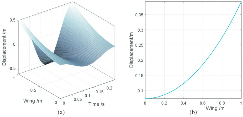
(a) (b)
Figure 1. The wing deformation curves during a vibration cycle and att= 0.03 s.
4. SIMULATION AND MEASUREMENT
According to the data given in [13], wing length L = 1 m, the frequency of the first vibration mode f1 = 5 Hz, frequency of forced vibration frequencyf=4 Hz, and amplitude of forced vibrationω0=0.1 m. The wing deformation curves during a vibration cycle and att= 0.03 s are demonstrated in Fig. 1.
All simulations are carried out in a uniform linear array of 8 elements with one half-wavelength inter-element spacing. The wavelength λ=0.2 m. The elements of the array are evenly distributed over thex-axis, and the first one is atx= 0 m. The Matlab program is established to simulate the uniform linear array receiving signals from different azimuth. When the array is deformed as shown in Fig. 1, there will be great errors if the MUSIC algorithm is used to estimate the azimuths of the signal sources directly. So in these simulations, we have applied the algorithm proposed in this paper to calibrate the errors. The τ in step 6 is generally set to 0.002◦ and εset to 1.
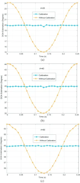
Considering the signal model mentioned above, the SNR of signal source is 20 dB, and the number of snapshotsK is 300. The DOA estimation angles calibrated have been obtained for different incident directions [20◦,40◦,60◦] in a vibration cycle. Compared with the MUSIC method without calibration, these calibrated DOA estimation angles are shown in Fig. 2.
From Fig. 2, we can see that this proposed method has a good calibration effect for different incident directions when the wing is on different deformation stages.
Figure 3 shows DOA estimation angles with and without calibration over 300 Monte Carlo experiments. The number of snapshotsK is 200. The incident direction of the signal source is 45◦, and the array deformation time is selected at 0.03 s. From Fig. 3, we can see that the error range is about [−0.1◦,0.1◦]. Considering that the systematic error (such as the step length) is about [−0.06◦,0.06◦], it can be concluded that the proposed method has good stability.
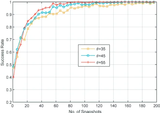
It is assumed that the error range of successfully estimated angle is [−0.2◦,0.2◦]. Fig. 4 shows the DOA estimation success rates at different SNRs for different arrival directions while the number of snapshots K= 300. The DOA estimation success rates against the numbers of snapshots are shown in Fig. 5 for different arrival directions when the SNR of signal source is 20 dB. The direction of incidence of the source is [35◦,45◦,55◦].
(a)
(b)
(c)
Figure 3. The DOA estimation angles over 300 Monte Carlo experiments.
Figure 4. The DOA estimation success rates of the proposed method for different SNRs.
5. CONCLUSIONS
In this paper, a gain-phase error calibration method for wing conformal array based on shape fitting is proposed. Compared with the other calibration techniques, the proposed method has the benefit that the obtained wing deformation data are not azimuth dependent. Additionally, it has great flexibility in implementation. The simulation results reveal that the accuracy and stability of the proposed method can be guaranteed. Since it can accurately reproduce the deformed shape of the conformal array, it is desirable to be applied in the analysis applications of conformal arrays.
ACKNOWLEDGMENT
This work was supported by the National Natural Science Foundation of China (No. 61571356).
REFERENCES
1. Qian, C., L. Huang, and H. C. So, “Computationally efficient ESPRIT algorithm for direction-of-arrival estimation based on Nystr¨om method,”Signal Processing, Vol. 94, No. 1, 74–80, 2014. 2. Mavrychev, E. A., V. T. Ermolayev, and A. G. Flaksman, “Robust Capon-based direction-of-arrival
estimators in partly calibrated sensor array,” Signal Processing, Vol. 93, No. 12, 3459–3465, 2013. 3. Ng, B. C. and C. M. See, “Sensor array calibration using a maximum-likelihood approach,” IEEE
Trans. Antennas Propag., Vol. 44, No. 6, 827–835, 1996.
4. See, C. M. and B. K. Poth, “Parametric sensor array calibration using measured steering vectors of uncertain locations,” IEEE Trans. Signal Process., Vol. 47, No. 4, 1133–1137, 1999.
5. Leshem, A. and M. Wax, “Array calibration in the presence of multipath,” IEEE Trans. Signal Process., Vol. 48, No. 1, 53–59, 2000.
6. Wang, B. H., Y. L. Wang, and H. Chen, “Array calibration of angularly dependent gain and phase uncertainties with instrumental sensors,”Sci. China Ser. F Inf. Sci., Vol. 47, No. 6, 182–186, 2003. 7. Friedlander, B. and A. J. Weiss, “Eigenstructure methods for direction finding with sensor gain
and phase uncertainties,” Circuits Syst. Signal Process., Vol. 9, 272–300, 1990.
8. Wijnholds, S. J. and V. D. V. Alle-Jan, “Multisource self-calibration for sensor arrays,” IEEE Trans. Signal Process., Vol. 57, No. 9, 3512–3522, 2009.
9. Weiss, A. J. and B. Friedlander, “Array shape calibration using sources in unknown locations — A maximum likelihood approach,” IEEE Trans. on ASSP, Vol. 37, No. 12, 1958–1966, 1989. 10. Wang, B. H., Y. L. Wang, and H. Chen, “Array shape calibration using carry-on instrumental
sensors,” Proceedings of the International Conference on Radar (IEEE Cat. No.03EX695), 636– 639, Huntsville, 2003.
11. Flanagan, B. P. and K. L. Bell, “Array self-calibration with large sensor position errors,” IEEE Trans. Signal Process., Vol. 81, No. 10, 2201–2214, 2001.
12. Hong, J. S., “Genetic approach to bearing estimation with sensor location uncertainties,”Electron. Lett., Vol. 29, No. 23, 2013–2014, 1993.
13. Schippers, H., J. H. van Tongeren, and G. Vos, “Development of smart antennas on vibrating structures of aerospace platforms of conformal antennas on aircraft structures,”Proc. NATO AVT Specialists Meeting Paper Nr, Vol. 20, 2–5, Oct. 2006.
14. Schippers, H., J. V. Tongeren, P. Knott, P. Lacomme, and M. R. Scherbarth, “Vibrating antennas and compensation techniques research in NATO/RTO/SET 087/RTG 50,” Proc. IEEE Aerosp. Conf., 1–13, 2007.
15. Isernia, T., A. Massa, A. F. Morabito, and P. Rocca, “On the optimal synthesis of phase-only reconfigurable antenna arrays,” Proc. 5th EuCAP, 2074–2077, 2011.