A simple experimental procedure to quantify image noise in
the context of strain measurements at the microscale using
DIC and SEM images
L.L. Wang1, E. H´eripr´e1,a, S. El Outmani1, D. Caldemaison1, and M. Bornert2
1 Solid Mechanics Laboratory, CNRS UMR 7649, Department of Mechanics, ´Ecole polytechnique ParisTech, 91128 Palaiseau cedex, France
2 Laboratoire Navier, ´Ecole des ponts ParisTech, Universit´e Paris Est, Champs-sur-Marne, 77455 Marne-la-Vall´ee cedex 2, France
Abstract. Image noise is an important factor that influences the accuracy of strain field measurements by means of digital image correlation and scanning electron microscope (SEM) imaging. We propose a new model to quantify the SEM image noise, which ex-tends the classical photon noise model by taking into account the brightness setup in SEM imaging. Furthermore, we apply this model to investigate the impact of different SEM set-ting parameters on image noise, such as detector, dwell time, spot size, and pressure in the SEM chamber in the context of low vacuum imaging.
1 Introduction
Digital Image Correlation (DIC) applied to Scanning Electron Microscope (SEM) images is of interest to evaluate the strain fields at the scale of the microstructure and has been widely used for the last ten years in the context of micromechanical investigations of materials [1–4]. But care should be taken to the accuracy in the displacement measurements, especially when small strain (below 1%) are to be evaluated. Errors depend on many factors and are more difficult to control than in the context of macroscopic DIC using optical images. In addition to ”intrinsic” errors of DIC algorithms induced for instance by shape function mismatch [6] or inaccurate subpixel image restoration by inappropriate grey level interpolations [7], there are many potential sources of ”extrinsic” errors when using SEM images, such as the instability of the scanning due for instance to beam drift or fluctuations of digi-tal/analog converters used in the scan generators, undersampling induced by the discrepancy between spot size and pixel size, high image noise levels, magnification fluctuations and other geometric errors due to imperfect alignment and image distortion. Some of these errors have been investigated and pro-cedures to control or correct them have been proposed [2, 5]. An important study has been performed by Cornille [5] who proposed a procedure to calibrate a SEM and to control its geometric errors. How-ever, such a procedure is very time consuming and can hardly be used in practice in the context of in situmechanical testing [4], essentially because of the long integration time of SEM images: the recording of high definition images used in the context of a multiscale analysis often requires several minutes.
The aim of this paper is to present a simple method to characterize and quantify one of these ex-trinsic error sources: the SEM image noise, which induces errors in displacement evaluations by DIC algorithms which scale linearly with noise levels [8]. Indeed noise levels in SEM images can reach rather high levels with respect to optical images, acquired with conventional modern CCD cameras, in which noise levels are usually limited to one or two grey levels on a total of 256 levels (8-bits
cam-a e-mail:[email protected]
© Owned by the authors, published by EDP Sciences, 2010 DOI:10.1051/epjconf/20100640008
eras), and can even be smaller on high end cameras. With older SEMs such low levels could hardly be reached [2] during a single scan. Image averaging procedures could be adopted to reduce this noise, but image drift can then seriously limit the spatial resolution of the images. On more recent SEMs, image noise can be reduced to significantly lower levels thanks to, first, higher electron fluxes in the incident beam, especially in SEMs equipped with a field emission gun (FEG) and, second, to improved general efficiencies of the detectors. However, image noise still depends on many factors such as de-tector mode (secondary -SE- or back-scattered electrons -BSE-, in high or low vacuum conditions, or even in environmental mode), kinetic energy of incident electrons (voltage), intensity of the beam (controlled by spot size and gun apertures), dwell time, brightness and contrast setups of the detec-tors and the analog/digital converters, etc. In addition, as contrast in SEM images are essentially the consequence of complex interactions of electrons and matter, noise levels also depend on the material under investigation, and its surface preparation, and might evolve with time because of the evolution of the material. Finally, in low vacuum conditions (pressure in the chamber up to 150 Pa) or under environmental conditions (pressure up to 3000 Pa), interactions of the incident and emitted electrons with the molecules of the surrounding gas play a fundamental role in image -and therefore noise- gen-eration. Such complex phenomena need to be mastered to optimize parameter settings. Though the skill of an experienced microscopist is essential to obtain good images, it might also be useful to build quantitative models to predict image properties as a function of setting parameters, for first, a better understanding of the physical processes at the origin of image generation, and second, to optimize parameter settings. This is in particular of interest in the context of mechanicalin situtesting, where a compromise between image noise and acquisition time of high definition images needs to be defined.
The presented noise model is essentially a modified Poisson noise model, which states that stan-dard deviation of the signal scales as the square root of its statistical expectation. It is presented and validated in section 2 as an extension of a more standard noise model suitable to describe noise levels in optical images. Extensions are mostly relative to an offset linked to the brightness control. In section 3, the model is used to quantify the evolution of the number of electrons detected by the detectors for given grey levels, as a function of various SEM setting parameters. Section 4 is a short conclusion and a discussion of the limitations of the model.
2 SEM image noise
In optical camera or SEM images, grey levels reflect statistics of discrete events: photons or electrons received by the detector. As such, they carry an intrinsic noise, the standard deviation of which is proportional to the square root of its expectation, as standard statistics show. More precisely, ifNis the number of discrete events counted by the detector,E(N) its statistical expectation, thenσN =
√ E(N) is its standard deviation. Total noise results of the combination of this photon noise with other sources of noise, such as thermal and read noise. The relative proportions of each noise source depend on the acquisition conditions.
Total noise can be quantified by averaging a large number of images of a fixed device and com-puting average and standard deviation of recorded grey levels. This can be done globally, for all pixels of an image, or grey level per grey level or even pixel per pixel for a better characterization of noise. However, such a procedure may fail for SEM images because their recording is generally slow and suffers from beam drift with time passing and possible evolutions of imaging conditions. A less time-consuming method is proposed and turns out to be sufficient to seek the noise for each grey level (or narrow grey level interval), instead of for each pixel. This is based on the hypothesis that the same grey level for different pixels corresponds to the same amount of electrons detected, which carry the same statistical electron noise. Therefore, the noise investigation can be restricted to two imagesAand Band to plot the standard deviation of grey levels, which can be evaluated by the difference of the two images A−2B, for all pixels that have the same grey level average A+2B as a function of the latter. More specifically, the grey level at pixelxcan be given the formA(x)=E(A(x))+A0(x) whereA0(x) is the random noise to be characterized. If the two images are acquired with similar conditions, then E(A(x))= E(B(x)) and the difference isA(x)−B(x)=A0(x)−B0(x). Assuming independent and sta-tistically identical noises in the two images, one has simplyσA−B =
√
2σA =
√
assumption, the standard deviation can be evaluated from the standard deviation ofA−Bfor all pixels that carry the same average grey level A+B
2 . In addition, this average can be considered as a good eval-uation of the expectation ofE(A(x)), since usually grey level fluctuations remain small with respect to their average value. For higher noise levels, or in the case of small images for which the number of pixels carrying the same average grey level might be too small, this analysis might be performed for grey level intervals: the standard deviation of the grey levels for all pixels whose average A+2Bbelongs to a given interval is then plotted against the center of this interval.
It should be noted that the analysis has to be restricted to pixels for which grey levels are not saturated. Indeed, ifAandBbelong to [0,Amax], one has−A+2B ≤ A−2B ≤ A+2B and A+2B−Amax≤ A−2B ≤ Amax− A+2B. So noise levels are only accurately evaluated at pixels for which the differenceA−B is strictly inside these intervals. Pixels which do not satisfy these conditions are removed from the analyses. Figure 2 illustrates this remark: each blue dot corresponds to a couple (A+2B,A−2B), while the red line gives the standard deviation. The blue cloud is bounded by the green lines corresponding to the above intervals and the red line can not be evaluated for grey level for which the blue cloud attains the green bounds. Another difficulty might be induced by small evolutions of imaging conditions between the recording of image A and B, which might modify grey scales between the two images, or induce a spatial shift of the second image with respect to the first one. Some specific algorithms might then be used to adjust the grey scale of the second image to the first one, and/or to associate corresponding pixels in the two images. For the sake of brevity, these procedures won’t be described here.
2.1 Photon noise in camera images
In optical camera imaging, grey levels are estimated by conversion of electric charges proportional to the amount of photons which are detected by the photoactive region of the CCD (charge-coupled device). This conversion can be expressed as:
S(X,T)=c(T)×N(X,T) (1)
whereS(X,T) is the grey level of the pixelXfor an integration timeT, andc(T) a conversion factor that linksS(X,T) to N(X,T), the number of photons received by the detector, which is a random variable. Therefore, the camera image carries a statistical photon noise, which can be described by the Poisson process: if ¯Nphotons arrive at a point (for the digital image, it is the pixel) in a given time T on the average, the fluctuations should be around
√
¯
N. Therefore, a classical photon noise model presenting optical image noise is:
σh
S(X,T)i=
q
c(T)×EhS(X,T)i (2)
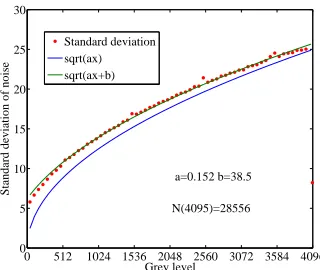
whereσ(S(X,T)) is the standard deviation of the grey level at pixel position Xwhich quantifies its noise level and E(S(X,T)) is the statistical expectation of its grey level. In this model, the standard deviation of grey level is the square root of its mean value, and this has been confirmed by the experi-mental results shown in figure 1, obtained from the analysis of two consecutive images recorded with a 12-bits 16 Mpixel camera, whose CCD sensor (Kodak KAI 16000) has aNmax=30000 electrons saturation signal. The noise curve measured with the above described procedure nicely fits the photon noise model, including in terms of numbers of electrons at saturation, as the interpolation of measured curve corresponds toNmax=28556 electrons. The only discrepancy is observed for low grey levels: the experimental curve does not start from zero. This is attributed to the other noise sources such as thermal or read noise. Under the present acquisition conditions, it is however noted that these other sources of noise can be neglected with respect to photon noise, as illustrated by the difference between the blue (photon noise only) and green (total noise) curves. Remark also that the last point of the curve corresponding to the maximal grey level is false because of the above mentioned saturation effects.
2.2 SEM image noise model
0 512 1024 1536 2048 2560 3072 3584 4096 0
5 10 15 20 25 30
Grey level
Standard deviation of noise
Standard deviation sqrt(ax) sqrt(ax+b)
N(4095)=28556 a=0.152 b=38.5
Fig. 1. Photon noise in a 12-bits camera image
0 64 128 192 256
0 5 10 15 20 25 30 35
Grey level
Noise
(A−B)/2 Standard deviation Noise saturation
Fig. 2. Noise in a 8-bits SEM image
from a secondary electron mode image in high-vacuum condition shows that the classical photon noise model does not describe the SEM image noise anymore. Unlike camera images, the image contrast and brightness setup can be modified in a wide range with strong consequences on image and noise levels. This can be performed at the level of the detector itself (e.g. by the application of a polarization voltage on the scintillator of the SE detector) or at the level of the electronic signal amplifiers. A consequence of this fact is that a zero grey level in an image might not coincide with the absence of electrons on the detector, or more generally that grey levels are no longer directly proportional to electron counts. A new model [10] is thus proposed which extends the classical photon noise model by the addition of a coefficientb(T) which is linked to the image brightness setup. Taking into account the contrast and brightness setup during SEM imaging, an affine contrast/brightness setup model is applied to describe the conversion from physical signal to digital signal, and equation (1) is rewritten as:
S(X,T)=c(T)×N(X,T)−b(T) (3)
whereN(X,T) can be expressed as:
N(X,T)=b(T)+∆N(X,T) (4)
The coefficientb(T) is a constant which is independent of the pixel position and ∆N(X,T) is the fluctuation aroundb(T). This latter coefficient can be assimilated to the number of electrons received by the detector for a null grey level. Introducing the new conversion formula but still assuming that electron counts obey the Poisson statistics, the SEM image noise model becomes:
σ[S(X,T)]= pc(T)× q
EhS(X,T)i+c(T)×b(T) (5)
If we suppose that ∆N(X,T) << b(T), equation (5) can be linearized with respect to ∆E(bN((TX),T)) =
E(S(X,T))
c(T)b(T) in the form (see [10] for details):
σ
E[S(X,T)]=c(T)× pb(T)+ E
h S(X,T)i
2√b(T) (6)
For the SEM image noise, the relation between standard deviation and mean value of grey level thus reads √ax+b(equation 5) ora0x+b0with approximation (6). Note that figure 2 confirms the coher-ence with this approximation. By using equations 3, 5 and 6, the amount of electrons received by the detector corresponding to a grey level can be estimated:
for the SEM image noise model
√
ax+b by N(X,T)= b a2 +
S(X,T)
a (7)
and for the SEM image noise model a0x+b0 by N(X,T)= 1 (2a0)2 +
S(X,T)×2a0
The amount of electrons received can be used to optimize the SEM setting parameters as shown in section 3.2 owing to the advantage of this parameter: it represent the intrinsic statistical electron noise, that essentially generates the SEM image noise, regardless of contrast and brightness setup.
2.3 Validation with two different materials
The SEM image model validation was performed for a large number of images recorded with different SEM setting parameters and two different materials: a metallic material, the Ag/Fe blend (figure 3) and a geological material, the claystone (figure 4). The choice of these two materials will allow the validation of the model with two different types of images. The Fe/Ag specimen provides highly contrasted images due to the two phases Fe and Ag compared to claystone. Moreover, the images of claystone will be taken in low vacuum conditions, that means that there is an influence of the SEM chamber pressure on the quality of the image and on the number of electrons detected. For each specimen, a series of images were obtained with different dwell time keeping the other parameters constant. SEM images of Fe/Ag blend specimen have been taken with standard setting parameters for the metallic materials i.e. with secondary electron detector in high vacuum condition. As for claystone, images have been taken in low vacuum mode and with the back-scattered electron detector. The latter permits to have more contrasted images and low vacuum mode aims at imaging the specimen without any gold sputtering on its surface. These setting parameters have been chosen in such a way as to be conform with the parameters that will be chosen for the mechanical in-situ testing with DIC. For every conditions, brightness and contrast have been modified such that the grey levels spread over the full available range without saturation. The histograms of the images are presented in figures 3 and 4. It is noted that the peaks of histogram present always the same composition of material regardless their grey level that can be modified by contrast and brightness setup. For example, the two peaks correspond to Fe and Ag phases in image 3. This has been used to later estimate the amount of electrons corresponding to a certain composition of material.
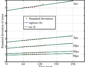
The noise model has been applied to images of these two materials taken with 5 different dwell times (figures 5 and 6). Remark that the image noise decreases with the dwell time. This is attributed to the increase of the number of electrons arriving for the same grey level with a longer dwell time. It is interesting to note that noise increases with the amount of electrons (correlated with the grey level) for a fixed dwell time, while it decreases with the electron number when dwell time varies. This is essentially due to the impact of contrast and brightness setup on noise amplitude, which can be explained by the model proposed. For a fixed dwell time, it is easy to note the noise increase with the grey level from equation 5 and 6. Besides, when we change the dwell time, it needs usually an adjustment of contrast and brightness to obtain a ”wide” histogram, and that would vary the noise amplitude as well. For example, there areN(t) electrons detected corresponding to a contrastc(t) for a pixel, and this number will reachnN(t) for a longer dwell time for the same pixel, therefore the contrast value has to be adjusted to c(nt) so as to obtain the same grey level (assuming for simplicity there is no brightness adjustment), which will reduce the noise from equation 5 and 6.
3 Application of the model
3.1 Evaluation of the amount of electrons captured by the detector
0 64 128 192 256 0
5000 10000 15000
Grey level Fe
Ag
Fig. 3. SEM image of Fe/Ag blend and its histogram, SE mode, high-vacuum condition, 20kV, spot 6
0 64 128 192 256
0 500 1000 1500 2000 2500 3000 3500
Grey level
Fig. 4. SEM image of claystone and its histogram, BSE mode, low-vacuum condition (35Pa), 10kV, spot 5.5
0 64 128 192 256
1 1.5 2 2.5 3 3.5 4 4.5 5 5.5
Grey level
Standard deviation of noise
standard deviation sqrt(ax+b) ax+b
40µs 20µs 10µs 1µs
5µs
Fig. 5. Standard deviation of noise of Fe/Ag blend images and validation of the noise model
0 64 128 192 256
0 1 2 3 4 5 6 7 8
Grey level
Standard deviation of noise
Standard deviation sqrt(ax+b) ax+b
1µs
5µs
10µs
30µs 50µs
Fig. 6. Standard deviation of noise of claystone images and validation of the noise model
3.2 Application of model to noise reduction
An important study has been performed by Doumalin [2], who investigated, by means real and sim-ulated images, the impact of image noise on the displacement measurement accuracy. The results showed an important error due to the image noise, as well as an increasing error with noise amplitude. More recent theoretical analysis confirm this tendency [8]. Therefore, it is necessary to reduce the image noise for the strain field measurement using DIC and SEM imaging, especially in microme-chanical investigations. Since the SEM image noise is essentially random, image averaging has been shown to be an effective method for minimizing the effect of noise: a smaller grey level and more images carry a lower noise level. Besides, imaging integration is also a direct-forward approach to reduce the noise. In this paper, we focused on another approach: optimizing the setting parameters of imaging. The model proposed in section 2.2 was applied to optimize the choice of setting parameters (dwell time, spot size and SEM chamber pressure in this study) for a claystone sample in low-vacuum condition.
As shown in the previous section, SEM image noise is essentially due to statistical electron noise. The number of electrons detected by the detector is an intrinsic factor that conditions the image noise am-plitude. As the study of impact of dwell time on noise in 2.3 has enhanced, the noise decreases with the amount of electrons detected for a given grey level. Therefore, the amount of detected electrons, which can be estimated by the model proposed, has been used as the parameter presenting SEM image noise level. A major advantage of this parameter is that it can eliminate the effect of the contrast/brightness setup, which might help to exhibit the intrinsic statistical electron noise.
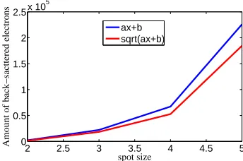
From figure 8 and 10, a longer dwell time and a larger spot size can remove the background noise in SEM images. This is attributed to the increase of the intensity of the electrons emitted by the interac-tion between primary electron and specimen. However, it is important to note that a long dwell time is not always favorable: the image acquisition time should be as short as possible in the context of in situmechanical testing in order to limit the specimen relaxation for instance, as well as the image shift accompanying a long image acquisition time. Compared with high-vacuum conditions, the noise level is higher in low vacuum condition for which the gas pressure in the specimen chamber plays an important role. The figure 9 shows that the noise amplitude increases with pressure, that can be readily attributed to the interaction between gas molecules and electrons.
4 Conclusions
In this paper, we showed the inadequacy of the classical photon noise model to describe the SEM image noise. A new model which takes into account the contrast and brightness setup is presented to qualify the SEM image noise. This model was validated by a large number of tests on two different materials. It can be used to fit the obtained data over a wide range of setting parameters.Furthermore, evaluations of amounts of electrons received by the detectors can be carried out by such a model. The influence of some setting parameters on the SEM image noise have also been studied. A longer dwell time and a larger spot size can reduce the image noise as long as the detector saturation effects are not encountered or image shift are not critical. Moreover, pressure of specimen chamber is also an important factor influencing the SEM image noise in low-vacuum condition. The next steps of this study will be the investigation of noise in environmental conditions, for which the presence of gas molecules is even more critical than in low vacuum conditions. Preliminary investigations show however that the proposed model might not be sufficient to characterize noise in such complex imaging conditions, as the assumption of independence of noise between neighbor pixels might not be satisfied. More sophisticated models might then be required.
5 Acknowledgments
The environmental FEG-SEM FEI Quanta 600 on which the images used in the present study were recorded was funded by the region ˆIle de France, through the SESAME 2004 program, CNRS and
´
0 10 20 30 40 0
1 2 3 4 5 6x 10
4
Dwell time (microseconds)
Amount of secondary electrons
ax+b sqrt(ax+b)
Fig. 7. Estimation of the amount of SE received by the detector during imaging of the Fe phase of the Fe/Ag blend
0 10 20 30 40 50
0 1 2 3 4x 10
5
Dwell time (microsecond)
Amount of back−scattered electrons
ax+b sqrt(ax+b)
Fig. 8. Estimation of the amount of BSE received by the detector during claystone imaging (value at peak of histogram)
20 30 40 50 60 70 80 90
0 0.5 1 1.5 2 2.5 3 3.5x 10
5
Pressure (Pa)
Amount of back−sacttered electrons
ax+b sqrt(ax+b)
Fig. 9. Evolution of the amount of electrons received with pressure - Back-scattered electron mode - Dwell time 30µs/pixel - Magnification
×2000 - Accelerating Voltage: 10kV - Spot 5.5
2 2.5 3 3.5 4 4.5 5
0 0.5 1 1.5 2 2.5x 10
5
spot size
Amount of back−sacttered electrons
ax+b sqrt(ax+b)
Fig. 10. Evolution of the amount of electrons received with spot size - Back-scattered elec-tron mode - Dwell time 30µs/pixel - Magnification
×2000 - Accelerating Voltage: 10kV - Pression 35Pa
References
1. L. Allais, M. Bornert, T. Bretheau, D. Caldemaison, Acta Metall. Mater.42, (1994) pp. 3865-3880. 2. P. Doumalin,Microextensom´etrie locale par corr´elation d’images num´eriquesPhD thesis, Ecole
Polytechnique (2000).
3. A. Tatschl and O. Kolednik, Mat. Sc. Eng. A339, (2003) pp. 265-280.
4. E. H´eripr´e, M. Dexet, J. Cr´epin, L. G´el´ebart, A. Roos, M. Bornert and D. Caldemaison, Int. J. Plasticity23, (2007) pp. 1512-1539.
5. N. Cornille,Accurate 3D Shape and Displacement Measurement using a Scanning Electron Micro-scopePhD thesis, Univ. South Carolina & Inst. Nat. Sciences Appliqu´ees Toulouse (2004). 6. M. Bornert, F. Br´emand, P. Doumalin, J.C. Dupr´e, M. Fazzini, M. Gr´ediac, F. Hild, S. Mistou, J.
Molimard, J.J. Orteu, L. Robert, Y. Surrel, P. Vacher, B. Wattrisse, Exp. Mech.49, 3, (2009), pp. 353-370.
7. Y. Q. Wang, M. A. Sutton, H. A. Bruck, H. W. Schreier, Strain,45, (2009), pp. 160-178 8. S. Roux and F. Hild, Int. J. Fracture140, (2006), pp. 141-157
9. https://www.lms.polytechnique.fr/users/bornert/CMV 14/.
10. S. El Outmani,Caract´erisation m´etrologique d’un microscope ´electronique `a balayage en vue de son utilisation pour la microextensom´etrieMaster thesis, Universit´e Paris Diderot (2008).