An Uncertainty Visual Analytics Framework for Functional Magnetic Resonance Imaging

(1)

i

A

N

U

NCERTAINTY

V

ISUAL

A

NALYTICS

F

RAMEWORK FOR

F

UNCTIONAL

M

AGNETIC

R

ESONANCE

I

MAGING

A thesis submitted to fulfil requirements for the degree of

Doctor of Philosophy.

Faculty of Engineering & Information Technologies

University of Sydney

Michael de Ridder

2018

(2)

ii

© Copyright by Michael de Ridder 2018

(3)

iii

Abstract

Improving understanding of the human brain is one of the leading pursuits of modern scientific research. Functional magnetic resonance imaging (fMRI) is a foundational technique for advanced analysis and exploration of the human brain. The modality scans the brain in a series of temporal frames which provide an indication of the brain activity either at rest or during a task. The images can be used to study the workings of the brain, leading to the development of an understanding of healthy brain function, as well as characterising diseases such as schizophrenia and bipolar disorder.

Extracting meaning from fMRI relies on an analysis pipeline which can be broadly categorised into three phases: (i) data acquisition and image processing; (ii) image analysis; and (iii) visualisation and human interpretation. The modality and analysis pipeline, however, are hampered by a range of uncertainties which can greatly impact the study of the brain function. Each phase contains a set of required and optional steps, containing inherent limitations and complex parameter selection. These aspects lead to the uncertainty that impacts the outcome of studies. Moreover, the uncertainties that arise early in the pipeline, are compounded by decisions and limitations further along in the process. While a large amount of research has been undertaken to examine the limitations and variable parameter selection, statistical approaches designed to address the uncertainty have not managed to mitigate the issues.

Visual analytics, meanwhile, is a research domain which seeks to combine advanced visual interfaces with specialised interaction and automated statistical processing designed to exploit human expertise and understanding. Uncertainty visual analytics (UVA) tools,

(4)

iv

which aim to minimise and mitigate uncertainties, have been proposed for a variety of data, including astronomical, financial, weather and crime. Importantly, UVA approaches have also seen success in medical imaging and analysis. However, there are many challenges surrounding the application of UVA to each research domain. Principally, these involve understanding what the uncertainties are and the possible effects so they may be connected to visualisation and interaction approaches. With fMRI, the breadth of uncertainty arising in multiple stages along the pipeline and the compound effects, make it challenging to propose UVAs which meaningfully integrate into pipeline.

In this thesis, we seek to address this challenge by proposing a unified UVA framework for fMRI. To do so, we first examine the state-of-the-art landscape of fMRI uncertainties, including the compound effects, and explore how they are currently addressed. This forms the basis of a field we term fMRI-UVA. We then present our overall framework, which is designed to meet the requirements of fMRI visual analysis, while also providing an indication and understanding of the effects of uncertainties on the data. Our framework consists of components designed for the spatial, temporal and processed imaging data. Alongside the framework, we propose two visual extensions which can be used as standalone UVA applications or be integrated into the framework. Finally, we describe a conceptual algorithmic approach which incorporates more data into an existing measure used in the fMRI analysis pipeline.

We evaluate our framework and visual extensions in different case studies using clinical fMRI data. In these we present case studies and expert feedback which highlight the benefits of the uncertainty visualisation, such as improved understanding, over existing statistical and visual approaches. Our proposed algorithmic approach was evaluated using classification, demonstrating improvements over the standardised alternative, and discuss

(5)

v

the implications of our conceptual method. The framework and extensions in this thesis therefore establish the fMRI-UVA research domain and advance the state-of-the-art in fMRI visual analysis.

(6)

vi

Acknowledgements

After writing so many words explaining the concepts in this thesis, I feel it best to keep the acknowledgements section short and to the point. Thank you to the following invaluable people.

To my supervisor, Jinman Kim, thank you for your time and dedication.

My auxiliary supervisor, Karsten Klein, a source of knowledge and perspective. Max Bennett, Jean Yang and Pengyi Yang for the fMRI data and analysis.

The fellow students and post-docs around me: Ashnil Kumar, Younhyung Jung, Lei Bi, Reza Zolfaghari, Tian Xia, Osmond Ahn, Robin Huang, Ha Phan, Hoijoon Jung, Yan Ke and David Lyndon.

Of course there are more transient colleagues, Mohib, Liviu, Falk, Florian, Yan and Pradeeba among others.

(7)

vii

List of Tables

Table 2.1: Summary of limitations in fMRI scanner hardware. ... 26 Table 7.1: Leave one out classification results for image comparison measures against Pearson's correlation coefficient. ... 141 Table 7.2: Leave three out classification results for image comparison measures against Pearson's correlation coefficient. ... 142 Table 7.3: Leave ten out classification results for image comparison measures against Pearson's correlation coefficient. ... 143

(16)

xvi

List of Figures

Figure 2.1: Functional magnetic resonance imaging pipeline (fMRI data flows from top to bottom). Raw data are acquired and processed in the first phase prior to data reduction or algorithmic image analysis. The results of the first two phases are visualised and

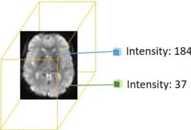
interpreted by humans. The interpretation is then used in a feedback loop to inform future studies which begin again at the top. ... 13 Figure 2.2: The attributes of a single volumetric image within the fMRI temporal

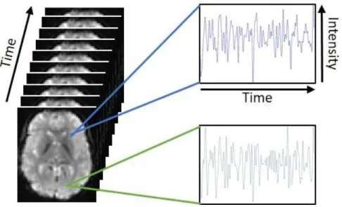
sequence. The volume is made up of voxels, which each have their own intensity value for that time point. ... 15 Figure 2.3: Illustration of the temporal aspect of fMRI. Each voxel has an intensity value at each time point which creates a time series of activity. ... 16 Figure 2.4: Demonstration of the uncertainty that arises in creating representative

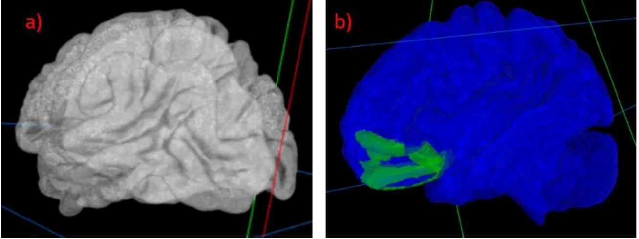
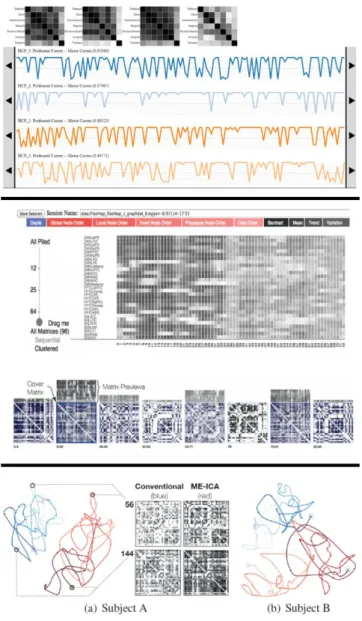
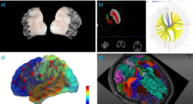
temporal signals. Multiple, potentially very different, voxel signals are summarised into a single representative signal that does not retain the variability. ... 29 Figure 2.5: An example of an fMRI visualisation using SPM [72] showing the results of white matter (WM), grey matter (GM) and cerebrospinal fluid (CSF) after segmentation with FSL FAST [64]: (a) the original fMRI image with a voxel size of 2x2x2mm; (b) the image with the uncertain, calculated matter types overlaid in shades of yellow (WM in the dark yellow; GM in the middle yellow; CSF in the bright yellow). ... 33 Figure 2.6: Examples of abstraction visualisations which focus on the temporal aspects of the data. Images created using – Left: TimeCurves [74]; Middle: SmallMultipiles [51]; Right: TemporalTracks [35]. ... 35

(17)

xvii

Figure 2.7: Examples of visualisations designed to target human interpretation issues, such as with spatial understanding and cognitive load. Images created using – a)

PyCortex [77]; b) CereVA [80]; c) BrainNet Viewer [81]; and d) Braviz [79]. ... 37 Figure 4.1: Example node-link diagram combined with a 3D anatomy of the brain,

created in BrainNet Viewer [81]. Edges have been thresholded to the top 10% of

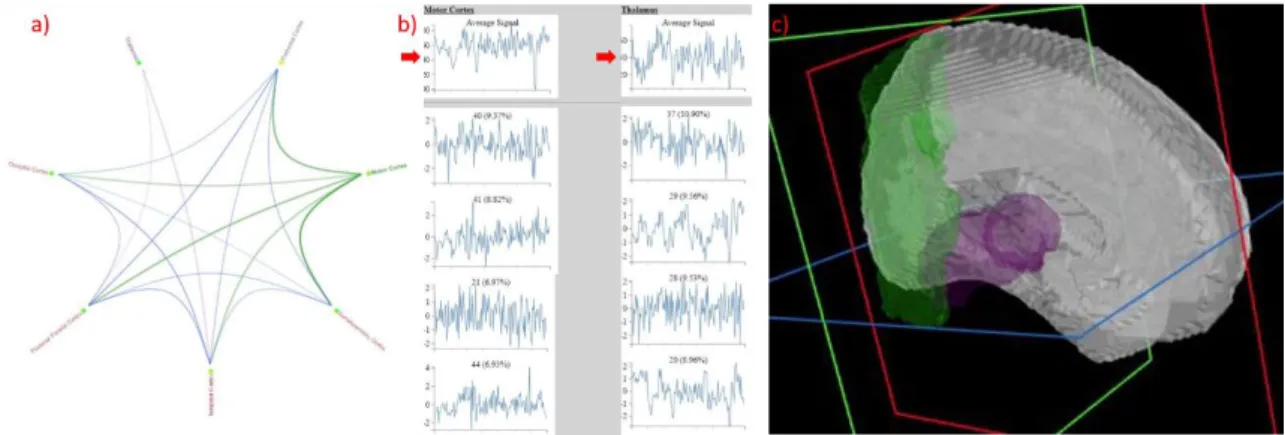
coactivation values (greater than 0.4) however the view is still cluttered. ... 47 Figure 4.2: Overview of our visual analytics framework. The core interface shows the three proposed components for: a) functional connectivity, with indicators for

thresholding and heterogeneity issues; b) anatomical context; and c) temporal sequences, which can show artifacts in the imaging data. The pop-outs to the side show how these components can be replaced in the framework. ... 52 Figure 4.3: (a) Illustration of node ordering on the radial. Right hemisphere regions are on the right, left hemisphere on the left and central regions in the middle. (b) The effects of edge bundling on the visual clutter, left has edge bundling and shows a clear pattern, while the right does not and the pattern is much harder to discern. ... 54 Figure 4.4: Anatomical views available in the framework. Rendering of the brain surface, split into left and right hemispheres in (a), and rendering of all the regions of interest in the brain, with one region highlighted in (b). ... 55 Figure 4.5: Small multiples view showing four subject FCNs at the same threshold clearly indicating the high-level differences that are visible in this view. ... 56 Figure 4.6: Illustration of the marker creation process and application. Multiple subject networks are selected to be added to the marker as shown at the top. Once applied to a different network, the highlighting denotes the relationship between the marker and that network. In this illustration, orange is for edges above the marker, blue for edges below and yellow for edges within the marker range. ... 57

(18)

xviii

Figure 4.7: The two versions of threshold bar with a grid added in red above the bars to indicate the division of the buckets. Top: in single subject mode; and bottom: in small multiples mode with 4 subjects selected. The bottom bar has been stretched vertically for more visual clarity and is best used with fewer subjects in the framework. ... 58 Figure 4.8: Comparison of the heterogeneity indicators in absolute and relative mode for a range of ReHo values. ... 59 Figure 4.9: The list of all the line profiles detected for a subject, shown when no node is selected. ... 60 Figure 4.10: The radial graph after the Motor Cortex has been selected in single select mode. The connected edges within the current threshold are highlighted. ... 62 Figure 4.11: Illustration of the visual changes that take place on double selection: (a) the edges on the radial are highlighted in two colours for the Motor Cortex and Thalamus; (b) the line profile container lists the average profile for each of the selected regions and the ordered list of profiles within the region; and (c) the anatomy viewer displays the two selected regions, but not the connected regions to avoid visual clutter. ... 62 Figure 4.12: Edge hover tooltip which displays the name of each node and the calculated coactivity value between them. ... 63 Figure 4.13: Demonstration of edge filtering. Left and right are the same network at the same threshold; right has had the edges connected to the Prefrontal Cortex filtered. ... 64 Figure 4.14: Drag and drop operation being performed to reorder the line profiles so comparison can be made more easily between profiles of interest. ... 65 Figure 4.15: Single colourised slice of the parcellation used; created as described in Woodward et al. [62] from the Harvard-Oxford cortical and thalamic parcellations. Green: Prefrontal Cortex; Yellow: Motor Cortex; Blue: Somatosensory Cortex; Pink:

(19)

xix

Temporal Cortex; Purple: Posterior Parietal Cortex; Red: Occipital Cortex; White:

Thalamus. ... 66 Figure 4.16: Overview for a healthy subject that is unexpectedly sparse at the high default threshold with two regions selected that have an incongruously high coactivation. In (a) the two regions are shown to be adjacent; (b) shows that the two average signals have out-of-scale peaks near the end; and (c) shows the sparse FCN and the high coactivation between the motor cortex and somatosensory cortex (indicated by the red arrow)... 68 Figure 4.17: Small multiples of the average healthy FCN (top-left) and five individual health patients; used to assess the accuracy and quality of the average FCN. The top two have a similar pattern to the average (determined by visual inspection), while the bottom three have a distinctly different pattern at the same threshold range. ... 70 Figure 4.18: Using the marker function to investigate a single schizophrenia subject. The marker was created using ten other schizophrenia patients, all with similar FCNs. The threshold bar has been set to a low range to observe the less coactive regions. ... 71 Figure 4.19: A threshold heatmap from a schizophrenia subject that is very tightly

clustered at a very high range. ... 72 Figure 4.20: The average activity profiles of the seven regions in the parcellation for one subject. All profiles contain similar drops at the end of the temporal sequence indicating an issue in the data integrity that can be explored in the other interface components, such as the homogeneity cues. ... 72 Figure 4.21: Removal of uncertainty caused by outlier time points which are visible on the line profiles (red boxes) for a subject diagnosed with schizophrenia. The original radial on the left is extremely dense, which is uncharacteristic for schizophrenia, while the radial on the right, after removal, is much more sparse, which is indicative of

(20)

xx

Figure 5.1: The standalone TemporalTracks interface: (a) subject selection panel; (b) subject functional connectivity networks visualised as matrices; (c) core tracks metaphor comparing the coactivation of the Prefrontal Cortex and Motor Cortex of six images; (d) the transition image for HCP_0, with a relatively speckled pattern; (e) difference mode selector, set to segment; (f) window size, set to 200 of a possible 1200 for these images; and (g) number of tracks, set to 11. In this example, it is visually clear that despite the correlations of HCP_1 and HCP_2 being similar (0.87 and 0.88, respectively), HCP_1 is much more coactive over the displayed time points, whereas HCP_2 has bursts of high coactivity and possible outliers that inflate the overall value. In comparison, HCP_4 has a slightly lower coactivation, yet a user can see that the early portion is much more stable in high coactivity than the later portion. Meanwhile, HCP_0, 2 and 6 all have lower

coactivation, which is mirrored by the numerous changes along the tracks. ... 87 Figure 5.2: Graphical definition of the tracks metaphor: (a) two modes of point difference and segment difference; (b) track placement; (c) example of point and segment

differences alongside the track placement diagram. ... 89 Figure 5.3: Creation of a transition image slice from two source image slices. The

absolute voxel-wise difference between the slices is taken. Therefore higher intensity spots in the transition image highlight areas of larger temporal variability. ... 90 Figure 5.4: Interaction with TemporalTracks: a) Shifting the top track left to compare it with a similar section of the bottom track; b) Dragging in from the right to compare a subset of temporal points; c) The same segment viewed on three, seven and eleven tracks; d) Illustration of exact and partial pattern matching; and e) Example of the changes that occur to the FCNs when shifting, dragging and window size adjustments are made. ... 92 Figure 5.5: TemporalTracks metaphor integrated into the uncertainty visual analytics framework for single select mode. The tracks are integrated into the time series

(21)

xxi

visualisation component (red box) allowing for comparison between the selected region and the connected regions. ... 94 Figure 5.6: TemporalTracks metaphor integrated into the uncertainty visual analytics framework for double select mode. Instead of listing multiple tracks, the direct

comparison between the two selected regions is shown instead of the average, with the signals that make up the regions listed below. ... 95 Figure 5.7: Summary of the case study results. (a) Highlighting some of the commonly repeated patterns. Beneath each of the tracks, a comparison to underlying BOLD shows that the same temporal coactivation patterns can look vastly different in the BOLD signals and that many of the patterns of interest do not occur only at high or low thresholds which are generally used to filter, e.g. in Liu et al. [64]; and (b) Some of the changes that occurred in the FCNs on interaction. These demonstrate the hemispheric symmetry. ... 98 Figure 5.8: Three examples of transition images demonstrating that the Human

Connectome Project Images contained a largely speckled pattern. ... 99 Figure 6.1: Main interface for the standalone implementation. Visualisation input

parameters are set above the small multiples grid which lists subjects down the page. .. 112 Figure 6.2: The meanings of the different graph elements. Colour is used to show the number of cores; size is used to denote the number of nodes; and a white circle with a black border separates the components. Components can have multiple cores, where the white is visible or they can have one core where only the black border is shown to save space. ... 115 Figure 6.3: Illustration of the small multiples grid. Each row is a subject and each column is a threshold value. ... 116

(22)

xxii

Figure 6.4: Illustration of the aggregation provided through hierarchical clustering. Five original subject rows are reduced to two through aggregation. Intermediate graphs are displayed along the dendrogram. ... 117 Figure 6.5: Threshold visualisation interaction examples. (a) Clicking to highlight similar decompositions; and (b) adjusting the minimum number of cores. ... 118 Figure 6.6: Demonstration of the extra information available using the k-core

decomposition graphs in the framework. Left shows the bucketed heatmap bar, which gives no indication to the underlying network, while right has the graphs for thresholds 0.5 to 0.95 in which connected component and topological properties are indicated on the circle packing diagrams (as described in Section 6.5.2). ... 119 Figure 6.7: Comparison of small world propensity (SWP) [149] and our proposed

visualisation approach in threshold selection. Threshold values are listed at the top of each column and SWP values are listed below each graph. SWP values of 0.6 are

considered to be small world by Muldoon et al. [149], yet a user is unable to tell networks apart with this value. ... 122 Figure 6.8: Comparison of small world propensity and our visualisation with the

Talairach parcellation [113]. ... 123 Figure 7.1: Creating images from the regional time series data using the Gramian Angular Field process. ... 131 Figure 7.2: The overall process used to create image functional connectivity networks.134 Figure 7.3: Nine example region Gramian Angular Field images from six subjects in the cohort. These images demonstrate a large amount of variability around the common grid structure that can be used in comparison. ... 138 Figure 7.4: Demonstration of encoding the temporal relationships and dependencies into the GAF images. The row indicated by the red arrow corresponds with the peak indicated

(23)

xxiii

by the other red arrow. Looking at the row, the similarity to all peaks and troughs along the time series is easily visible. Thus, this data, which would not be available in typical FCN creation, is included in image comparison methods without the need for extra

processing. ... 139 Figure 7.5: Examples of functional connectivity networks created with the different image comparison methods and Pearson's correlation. Each row is a subject and each column is a comparison technique. Looking across the rows, it is clear that some of the coactivity relationships stay very similar and stable across the methods, while others change quite a lot. ... 140

(24)

xxiv

List of Algorithms

(25)

xxv

List of Publications

The following publications were produced over the course of the candidature. Most of the publications were based on the research that is presented in this thesis. The lists include work which has been published, submitted, is under revision and is in preparation.

Journal Articles:

1. M. de Ridder, K. Klein, J. Yang, P. Yang, J. Lagopoulos, I. Hickie, M. Bennett, and J. Kim, “An uncertainty visual analytics framework for fMRI functional connectivity”, Neuroinformatics, 1-13, 2018.

2. M. de Ridder, K. Klein, and J. Kim, “A review and outlook on visual analytics for

uncertainties in functional magnetic resonance imaging”, Brain Informatics, 5(2), 5, 2018.

3. M. de Ridder, K. Klein, and J. Kim, “Interactive visually guided threshold

selection for fMRI functional connectivity networks,” NeuroImage, submitted, 2018.

4. M. de Ridder, K. Klein, and J. Kim, “ImageFCN: A method for creating robust

fMRI functional connectivity networks from image representations of the time series data,” ACM/IEEE Transactions on Computational Biology and Bioinformatics, in preparation, 2018.

Conference Proceedings:

5. M. de Ridder, K. Klein, and J. Kim, “Adapted K-Core Decomposition and

(26)

xxvi

Networks”, Engineering in Medicine and Biology Society (EMBC), 2018 40th Annual International Conference of the IEEE, under review, IEEE, 2018.

6. M. de Ridder, K. Klein, and J. Kim, “TemporalTracks: Visual analytics for

exploration of 4D fMRI time-series coactivation,” Proceedings of the Computer Graphics International (CGI) Conference, pp. 13-19, ACM, 2017.

7. M. de Ridder, Y. Jung, R. Huang, J. Kim, and D. Feng, "Exploration of virtual and augmented reality for visual analytics and 3d volume rendering of functional magnetic resonance imaging (fMRI) data," Big Data Visual Analytics (BDVA), pp. 1-8, IEEE,2015.

8. M. de Ridder, K. Klein, and J. Kim, "CereVA-Visual Analysis of Functional Brain Connectivity," International Conference on Information Visualization Theory and Applications (IVAPP), pp. 131-138, 2015.

(27)

xxvii

Abbreviations

2D Two Dimensional

3D Three Dimensional

4D Four Dimensional

AAL Automated Anatomical Labeling

ADHD Attention Deficit Hyperactivity Disorder AFNI Analysis of Functional NeuroImages BOLD Blood Oxygen Level Dependent CSF Cerebrospinal Fluid

CSS Cascading Style Sheet

D3 Data-Driven Documents

DICOM Digital Imaging and Communications in Medicine

DMN Default Mode Network

DTI Diffusion Tensor Imaging

FCN Functional Connectivity Network

fMRI Functional Magnetic Resonance Imaging

FMRIB Functional Magnetic Resonance Imaging of the Brain FSL FMRIB analysis group Software Library

GAF Gramian Angular Field

GLCM Grey Level Co-occurrence Matrix

GM Grey Matter

HCP Human Connectome Project HTML HyperText Markup Language

(28)

xxviii ICA Independent Components Analysis MNI Montreal Neurological Institute MUTI Mutual Information

NIfTI Neuroimaging Informatics Technology Initiative PCA Principal Components Analysis

PCC Pearson's Correlation Coefficient ReHo Regional Homogeneity

ROI Region of Interest

SIFT Scale Invariant Feature Transform SPM Statistical Parametric Mapping SSIM Structural Similarity Index SVG Scalable Vector Graphics SWP Small World Propensity

TR Repetition Time

UVA Uncertainty Visual Analytics

VMAR Virtual, Mixed and Augmented Reality

WM White Matter

(29)

1

Chapter 1 Introduction

Surface visualisation of the brain with posterier-ventral part of the cingulate gyrus in green and the lingual gyrus in red from the Destrieux parcellation.

(30)

2

1.1. Summary

Developing an understanding of how the brain functions is one of the main efforts of enquiry in medical research today [1-5]. International projects such as the Human Connectome Project [6] and The Brain Initiative [7] highlight the size and scope of endeavours. These efforts seek to map out and understand how the brain works in different situations, e.g. at rest and when performing tasks, and the differences between healthy and diseased brains. To learn and discover this information, the medical imaging modality of functional magnetic resonance imaging is used extensively. Analysis of the images involves transforming multifaceted, complex, and not well understood data into meaningful information that can be interpreted. However, the process undertaken to perform this transformation introduces a range of data and human uncertainties. Data uncertainties arise from difficulties such as inherent limitations in the acquisition and processing of the images, and the need for complex parameter selection. Human uncertainties, meanwhile, relate to the researcher’s ability to understand and interpret the complex information, while accounting for data uncertainties and cognitive load. These limitations prevent wider application and understanding of the data. Visual analytics is the process of transforming data into an interactive visual form that enables analytical reasoning. It can be used to expose both important and incomplete information to aid human interpretation. Visual analytics for brain research is a rapidly growing field that promises to assist in transforming and interpreting the uncertainty filled data. This thesis aims to facilitate visual analytics of such uncertainty, thus enabling new insights, applications and interpretations of the data. This chapter presents an introduction to the overall problem that we aim to address in this thesis, we then formalise these aims and list the main contributions we achieved. Finally, we present a guide to the organisation of the thesis.

(31)

3

1.2. Motivation

Functional imaging technologies that measure changes in metabolism, blood flow, chemical composition and absorption are fundamental to modern medical research. Functional magnetic resonance imaging (fMRI) is a four-dimensional (4D) medical imaging modality that is used to scan changes in brain activity over time [8]. The modality consists of three spatial dimensions, of tens to hundreds of thousands of voxels, and one temporal dimension, containing intensity values for each voxel, representing the activity. These temporal data collectively represent the functioning of the brain over time. The usefulness of this modality has greatly increased the understanding of the neural system; however, the acquisition of this imaging data is only the first step in the research procedures. To achieve the goals of brain research, vast efforts have been made into developing new methods to gain meaning out of fMRI, e.g. [9-17]. Visual analytics is vital to multiple steps in the processes, where it assists in effectively analysing and interpreting the data as it is transformed [18].

Studies of fMRI are interested in the relationships between voxels and regions in a single brain, as well as the associations between multiple brains [18-22]. These relationships occur over the temporal dimension and are rooted to a spatial location for the full time-course and for subsets of time. Thus, researchers require the ability to explore patterns and derived information for single images, groups of images, and when comparing images [18-22]. Moreover, information must be gathered while processing the data that contributes to decision making by researchers in algorithm and parameter selection [17, 18, 23-26]. Supporting these tasks relies on presenting valuable information derived from the volumetric and temporal data, as well as an indication of potential uncertainties in the data and processes [17, 23, 26]. These uncertainties arise from inherent limitations in both the

(32)

4

data acquisition and image processing algorithms, unknown considerations relating to human biology, the manual selection of options and parameters in processing the images, and the cognitive impacts of such complex data during processing and interpretation [18, 23, 26]. Many of these uncertainties impact the quality of the data in both the spatial and the temporal domains and thus compound upon one another. As a result, multiple concerns have arisen about the results of fMRI analysis in understanding brain function, e.g. [23-33]. Overcoming these concerns is arguably the biggest challenge in functional brain research and has prevented advances in fMRI application, such as clinical use [17, 19, 29, 32]. In addition, these concerns have negatively influenced the reputation of fMRI meaning that important findings can be overlooked by researchers outside the domain [17-20, 27, 29, 34].

Consequently, the tremendous potential of fMRI and its analysis has not been fully realised in research and is largely unrecognised by clinical applications [17, 24]. One of the principal reasons for this lack of uptake is that observing many of the uncertainties currently requires a great deal of expertise due to an absence of tools to interpret these uncertainties alongside analysis of the data. Current visual analytics tools are dominated by visualisations of just the derived information [18]. In such approaches researchers must manually observe, interpret and react to possible uncertainties in the data without any guidance. This is a subjective process with heavy reliance on the skills and experiences of the users and can be strongly impacted by bias or expectation, e.g. of functional characteristics [18, 27, 29]. Meanwhile, visual analytic tools developed for interpretation of the derived information do not consider the decisions made during the processing stages [18, 35, 36]. As a result, researchers are unable to gather information on potential issues and confounders in the data. Instead, the visual analytics tools focus on reducing cognitive

(33)

5

load and increasing the understandability of the derived information [18]. While these are crucial factors that are paramount to correct interpretation, the available tools do not present the whole picture of the data and analysis is thus limited.

The processes associated with transforming the fMRI data to significant information have meanwhile matured to the point where it is now a largely standardised pipeline [17]. Visual analytics tools can accordingly be developed to target aspects of this pipeline and the information presented at the culmination of the process. This enables the development of a visual analytics framework to assist in minimising the impact of uncertainties that integrates into the pipeline. Doing so fills a clear gap in the research of brain function. The advancement and application of visual analytics to this problem has the potential to expand the capabilities of fMRI research, making it a clinically viable tool because the uncertainties in the data become understood factors that users can adjust for.

1.3. Aims

The overall aim of the research presented in this thesis is to establish a framework for the visual analysis of fMRI with respect to the uncertainties that arise throughout the pipeline. We term this domain fMRI-UVA for functional magnetic resonance imaging uncertainty visual analytics. The framework will consist of complimentary components designed to expose uncertainties in the pipeline and in the derived information, while still reducing the cognitive load on users and increasing the understandability of derived information. Achieving this overall aim will require the fulfilment of the following specific sub-aims:

1. The creation of an overall visual schema for visualisation and interaction with information derived from the fMRI data. This schema will be designed to balance

(34)

6

the needs of the user in understanding and interpreting the meaning of the derived information with the impact of the uncertainties.

2. The development of specific visual analytic tools to be used in the overall schema and during the pipeline that provide insight into uncertainties in the data without compromising the currently available information about the data itself

3. The establishment of an understanding of uncertainties in the fMRI analysis pipeline with respect to how visual analytics can be leveraged in understanding and minimising their impact.

1.4. Contributions

To address the above aims, this thesis proposes a novel framework for fMRI-UVA and contains the following innovative contributions:

1. Chapter 2: Formalisation of the fMRI analysis pipeline with respect to the uncertainties and visual analytics.

We examine the fMRI analysis pipeline and existing visual analytics approaches to create connections between data and human uncertainties and visual analytics techniques. This is the first work to define and establish the relationship between fMRI uncertainties and visual analytics; including categorising the pipeline into three distinct steps which can be addressed with visual analytics. As a result, existing visualisation approaches focussed on human understanding alone. This is a major step as future advances can target specific uncertainties based on our research to mitigate issues in fMRI analysis. The review carried out to connect the fMRI pipeline to uncertainties and visual analytics led to the following publication:

(35)

7

 M. de Ridder, K. Klein, and J. Kim, “A review and outlook on visual

analytics for uncertainties in functional magnetic resonance imaging”,

Brain Informatics, 5(2), 5, 2018.

2. Chapter 4: Framework for visual analysis of fMRI information which integrates details related to uncertainties for interpretation.

The proposed framework sets up a visual analytics schema for the exploration of fMRI data with awareness and interpretation of both the human and data uncertainties. Interactions between the spatial, temporal and abstract dimensions of the data are accounted for in different visual components. This framework is a substantial advancement over existing approaches which only consider the human uncertainties when presenting the data. Moreover the extensibility as a framework rather than a standalone tool allows for integration with future developments. This framework has led to the following publications:

 M. de Ridder, K. Klein, J. Yang, P. Yang, J. Lagopoulos, I. Hickie, M. Bennett, and J. Kim, “An uncertainty visual analytics framework for fMRI functional connectivity”, Neuroinformatics, 1-13, 2018.

 M. de Ridder, Y. Jung, R. Huang, J. Kim, and D. Feng, "Exploration of virtual and augmented reality for visual analytics and 3d volume rendering of functional magnetic resonance imaging (fMRI) data," Big Data Visual Analytics (BDVA), pp. 1-8, IEEE, 2015.

 M. de Ridder, K. Klein, and J. Kim, "CereVA-Visual Analysis of Functional Brain Connectivity," International Conference on

(36)

8

Information Visualization Theory and Applications (IVAPP), pp. 131-138, 2015.

An early prototype of our framework was also accepted as a special mention for Best Potential in the BioVis 2014 Data Contest, however we had to withdraw our submission due to inability to attend.

3. Chapter 5: Visual extension to the framework for exploring temporal uncertainty in fMRI.

Our innovative visual metaphor is designed to aid in understanding the temporal relationships of regions in the brain through coactivity analysis. This extension can be used as part of the overall framework and has been implemented as a standalone application. Our approach allows for exploration of local and global temporal data uncertainty. In contrast, the limited existing approaches only consider global temporal uncertainty and their interactions are not designed to mitigate the uncertainty. This contribution led to the following publication:

 M. de Ridder, K. Klein, and J. Kim, “TemporalTracks: Visual analytics

for exploration of 4D fMRI time-series coactivation,” Proceedings of the Computer Graphics International (CGI) Conference, pp. 13-19, ACM, 2017.

4. Chapter 6: Visual extension to the framework for guided selection of thresholds in fMRI analysis.

This extension is important for the selection of thresholds during fMRI analysis. Existing approaches are based on inaccurate and hard to distinguish statistics that do not give details about the underlying brain network. Our proposed visual

(37)

9

approach adds to the information available in statistical methods by providing network topology details important to threshold comparison and further analysis. This extension is important because thresholds are necessary in fMRI analysis, however they are very difficult to select and there are no accepted methods for defining appropriate threshold values. This extension can also be integrated into the framework and used as a standalone tool for exploring fMRI populations. This contribution led to the following publications:

 M. de Ridder, K. Klein, and J. Kim, “Interactive visually guided

threshold selection approach for fMRI functional connectivity networks,” NeuroImage, submitted, 2018.

 M. de Ridder, K. Klein, and J. Kim, “Adapted K-Core Decomposition

and Visualization for Functional Magnetic Resonance Imaging Connectivity Networks”, Engineering in Medicine and Biology Society (EMBC), 2018 40th Annual International Conference of the IEEE, under review, IEEE, 2018.

5. Chapter 7: Algorithmic extension to the framework for improved creation of functional connectivity networks.

The proposed algorithmic method for creating functional connectivity networks converts the fMRI time series of regions into images which represent the trends and relationships between individual temporal points and temporal subsets. Thus, more information is encoded into the image than the time-series. Further, the images can be compared using mature and advanced image processing algorithms, which have considerably more research behind them than fMRI coactivation measures. Thus, the advancement over existing approaches are in

(38)

10

the method itself and the broadened domain it becomes a part of. This contribution led to the following publications:

 M. de Ridder, K. Klein, and J. Kim, “ImageFCN: A method for creating

robust fMRI functional connectivity networks from image representations of the time series data,” ACM/IEEE Transactions on Computational Biology and Bioinformatics, in preparation, 2018.

1.5. Organisation of this Thesis

The remainder of this thesis is organised as follows. Chapter 2 gives an overview of fMRI as a medical imaging modality and introduces the range of data and human uncertainties that arise along the processing pipeline. In Chapter 3, we describe the fMRI datasets and visualisation environment for the proposed framework and extensions. Our proposed framework is presented in Chapter 4. We then discuss two visual and one algorithmic extensions to the framework in the next three chapters. Chapter 5 presents an extension for exploring and mitigating temporal uncertainty in fMRI. Chapter 6 explains an extension for visually guided threshold selection in functional connectivity analysis. The algorithmic extension, a method for creating functional connectivity networks by representing and comparing the temporal information as images, is described in Chapter 7. Chapters 4, 5, 6 and 7 are the core contributions of the thesis. Finally, Chapter 8 summarises the contributions and significance of this thesis and presents directions for future research.

(39)

11

Chapter 2 Background to fMRI and fMRI

Uncertainties

Comparison of four different parcellations: Talairach, Harvard-Oxford Cortical, Automated Anatomical Labelling and Harvard Oxford Subcortical. Each parcellation is

(40)

12

2.1. Summary

This chapter introduces the functional magnetic resonance imaging (fMRI) modality and its analysis pipeline with an exploration into uncertainties that rise along the pipeline. In this chapter we set the baseline and background knowledge that is required for fMRI uncertainty visual analytics (fMRI-UVA). To do so, we present the background alongside an examination of the uncertainties, which contains novel contributions in characterising and mapping the uncertainties for fMRI-UVA. Our discussion of the fMRI modality is not designed to be exhaustive; instead it is meant to act as an introduction to the technologies and processes underlying the research area of this thesis. The focus is on fundamental topics necessary for understanding the latter parts of this thesis, with emphasis placed on the characteristics of each uncertainty and how visual analytics can be applied. Moreover, the compound effects of uncertainties are also discussed. That is, events that occur in one phase of the pipeline directly impact later stages of the pipeline and the associated uncertainty. For a comprehensive explanation of fMRI and its analysis, we recommend the following books and papers: Introduction to Functional MRI Hardware [37], Functional Connectomics from resting-state fMRI [38], fMRI Techniques and Protocols [8], Review of Functional and Clinical Neuroscience [39], Networks of the Brain [21] and Overview of fMRI analysis [4].

2.2. Functional Magnetic Resonance Imaging Analysis Pipeline

Figure 2.1 illustrates an overview of the fMRI analysis pipeline. The pipeline consists of three phases: (i) acquisition and data processing; (ii) image analysis; and (iii) visualisation and human interpretation. Each of these phases contains multiple steps that will be described in the following sections.

(41)

13

Figure 2.1: Functional magnetic resonance imaging pipeline (fMRI data flows from top to bottom). Raw data are acquired and processed in the first phase prior to data reduction or algorithmic image analysis. The results of the first two phases are visualised and interpreted by humans. The interpretation is then used in a feedback loop to inform future studies which begin again at the top.

2.2.1 Data Acquisition and Image Processing

This section provides an overview of fMRI acquisition, fMRI data, and the immediate image processing steps that are taken.

2.2.1.1. Functional Magnetic Resonance Imagine Acquisition

Acquisition of fMRI is based on an indirect measure of neuronal activity. The concept states that when neurons are active, they require more energy, in the form of glucose, than

(42)

14

when they are inactive. Neurons that are more active, in turn require more oxygenated blood, because oxygenated blood carries the glucose. There are multiple methods for recording this glucose uptake; the most common being blood-oxygen-level-dependent (BOLD) contrast imaging, in which neurons with more oxygenated blood are less attracted by magnetism than neurons with less oxygenated blood.

Detection of fMRI data, therefore, relies on the magnetism of neurons. During acquisition, the patient lies inside an MRI scanner. This scanner emits extremely strong magnetic pulses towards the patient, from a full 360 degrees, and records the attraction of objects within, taking a snapshot of, e.g., the BOLD.

2.2.1.2. Functional Magnetic Resonance Imaging Data

The imaging modality is four dimensional, consisting of three spatial dimensions to represent the volume of the brain, and one temporal dimension that records the activity of the brain in each spatial location over time. Figure 2.2 shows the attributes of a single volumetric image within the temporal sequence. Each volume consists of discrete sample points known as voxels. Each voxel is represented by a grey-scale intensity value that is generated by reconstructing emissions that molecules and atoms within the body make under a strong magnetic field. The voxels are taken in a grid-like pattern, where each two-dimensional plane of the grid is referred to as a slice. The spatial resolution of these voxels refers to their size and is given in width × height × depth. For example, a voxel can have a spatial resolution of 1.0 mm × 1.0mm × 2.0mm, this voxel has a volume of 2.0 mm3.

(43)

15

Figure 2.2: The attributes of a single volumetric image within the fMRI temporal sequence. The volume is made up of voxels, which each have their own intensity value for that time point.

The temporal dimension of fMRI is made of a series of three-dimensional volumetric images. Each volume can be considered as a snapshot of the brain’s activity at a certain time. These volumes are either taken in sequential slices, i.e. 1, 2, 3, … N, or interleaved, i.e. 1, 3, 5, … (N-1), 2, 4, 6, … N. The time taken between imaging the same slice consecutive times, i.e. time between slice 1 in volume 1 and slice 1 in volume 2, is referred to as the repetition time (TR). The number of volumes in an fMRI sequence is appended to the number of voxels (slices) along each edge of the volume to give the spatiotemporal resolution in width × height × depth × volumes, e.g. 256 × 256 × 128 × 140. As a result, each voxel in each volume represents the activation of a small area of brain tissue at a specific time point. Connecting each activation value together in a sequence creates an activity curve, or timecourse, of the voxel. Figure 2.3 illustrates the temporal aspects of fMRI data.

(44)

16

Figure 2.3: Illustration of the temporal aspect of fMRI. Each voxel has an intensity value at each time point which creates a time series of activity.

2.2.1.3. Image Reconstruction and Refinements (Image Processing)

Acquired fMRI data requires multiple processing steps before it can be viewed, analysed and interpreted. The following will present an introduction to the main steps in the process. Note that further image processing also takes place in other parts of the pipeline; thus the steps here are related to image reconstruction and refinements.

Image reconstruction is the process of converting the raw data from the scanner, called k-space data, into four dimensional images. The k-k-space is the Fourier transform on the MRI, thus image reconstruction is based on Fourier transformation algorithms.

Motion correction is required because fMRI scans are taken over extended periods of time during which patients move. To ensure the same area of the brain aligns with the same voxel in all temporal volumes, a target volume is selected – often the first volume or a ‘standard space image’, however it can be any other volume, or an average of multiple time points – and all the other volumes are ‘registered’ to it.

(45)

17

A standard space image is one that has been created external to the study at hand and published so that it can be used by anyone to create a common brain volume by which to compare images and studies. Standard space images are mostly created by combining fMRI from multiple subjects into one average image. Resulting standard space images are a single volume (one time point), rather than a functional image (with multiple time points). The most widely used standard space image is MNI152 from the Montreal Neurological Institute [40].

Registration is designed to process two images so that they are spatially aligned, ensuring consistency between volumes in the temporal sequence, and between images when using a standard space. In registration, the source image is transformed to match the target image by means of global – e.g. scaling and rotating – and local transformations – e.g. warping certain voxels.

Slice timing correction is necessary because typical fMRI scanners take the volumetric images one slice at a time. Therefore, each slice in the grid is scanned at a slightly different time. Slice timing correction typically uses interpolation to estimate voxel intensity at the time-point of each volume or by utilising a model of expected function to adjust and shift the recorded intensity.

Spatial filtering is the process of adjusting the intensity value for each voxel using neighbouring voxels and a weighting defined by a 3D Gaussian function. The method is used to increase the signal to noise (SNR) ratio of the image.

Temporal filtering serves a similar purpose to spatial filtering for the temporal dimension. The fMRI time series for a voxel contains scanner and other physiological signals as well as the recorded BOLD signal. High pass filtering is used to remove low frequency signals,

(46)

18

such as trends in the time series; low pass filtering removes high frequency noise, such as fast peaks and troughs in the signal.

Global intensity normalisation is applied to all images used within a study, rather than a single patient image. It is used to normalise the mean voxel intensity for the whole dataset because each fMRI has a different mean intensity due to factors such as different patient physiology and other influences, e.g. caffeine levels.

Bias field correction is needed to counter variations in the magnetic field of fMRI scanners. These can be caused by, e.g. wear on the machine, small inconsistencies in electric current and other imperfections in the scanner hardware. Bias field correction estimates the changes in magnetic field using global and local voxel information, often from different tissue types in the brain, using these to adjust individual voxel values.

Background removal is used to ensure fMRI images only contain voxels that align with the brain. In the processing, the scanner bed and the skull are the most common background matter, although other scanner artifacts and physical objects may need to be removed.

Tissue segmentation is used to break the fMRI into subsections for the types of matter in the brain. Generally, the brain is considered to be made of white matter, grey matter and cerebrospinal fluid. Each of these has different spatial and intensity ranges that can be segmented apart. Similarly, tumours can be segmented as their activity is different to other brain matter.

2.2.2. Image Analysis

The second phase of the fMRI analysis pipeline is designed to transform the complex 4D data into a format that can be more readily understood and interpreted by humans. This transformation can be performed using a range of automatic and semi-automatic image

(47)

19

analysis methods. The most common of these methods perform data reduction to group the voxel-level and temporal information into classes, while others attempt to gain information by analysing the voxel-level data algorithmically, e.g. via machine learning.

2.2.2.1. Data Reduction Methods

Data reduction methods transform four-dimensional fMRI images into two- and three-dimensional formats. This can be done by grouping voxels based on anatomical location, temporal signal, or a combination of both.

Functional Connectivity Analysis is a method to perform data reduction based on anatomical location. The technique results in the creation of functional connectivity networks (FCNs) – sometimes called functional connectivity matrices – which are two-dimensional representations of fMRI data. Voxels are grouped into defined 3D regions of interest (ROIs) using pre-segmented atlases, known as ‘parcellations’. Representative temporal signals are then created for each ROI to reduce the multitude of temporal voxel signals a single signal. The most common techniques for creating a representative signal is through voxel averaging, however more advanced methods are occasionally used. After the application of a parcellation and grouping the voxels, the fMRI data has been reduced, however it is still four-dimensional. The final step in the process is to calculate the ‘coactivation’ of the ROIs. This is done by comparing the representative signal, typically via correlation, although more innovative methods can also be used. The resulting FCN is a 2D matrix of coactivation values where there is a value to represent each pair of ROIs. Consequently, FCNs can be thought of as fully connected networks that represent how similar pre-defined regions of the brain are over time.

Parcellations are brain atlases, commonly created with a standard space image, that are segmented into a set of anatomical regions. There are many parcellations

(48)

20

designed for different purposes and by different groups. ROIs in parcellations can be based purely on anatomical location, or they can be created in group-based studies from functional activity of connected regions.

Coactivation is the term given to how similar regions of the brain are over time.

Principal and Independent Components Analysis are two related methods that utilise the temporal and spatial data. Both approaches are widely used in statistics and other sciences for data reduction. For fMRI, they are used to group voxels into classes of similar function, where the grouping is subject-specific, rather than from a pre-defined source. The major drawback of this approach compared to using FCNs is the increased difficulty in comparing subjects, due to spatial mismatch of voxel groupings. However, the methods are still used to map to ‘known networks’, such as the default mode network, which is a set of voxel groups spread throughout the brain that are known to have similar activation during rest.

Amplitude of Low Frequency Fluctuations and fractional Amplitude of Low Frequency Fluctuations are used to measure spontaneous fluctuations in the BOLD signal intensity for a selected region or voxel. These methods are generally used in resting-state imaging.

Voxel clustering is normally based on the temporal signal. Common clustering techniques, such as k-Means clustering and hierarchical clustering, are run on the voxel data. The input vectors of the algorithms are the temporal intensity values, which results in a location-independent clustering; however, these can be weighted by the voxel neighbourhood to take the anatomical location into account.

Seed-based approaches are commonly used as secondary data reduction methods, in which they are used in combination with functional connectivity analysis. The purpose is to compare the representative signal from one or more regions to the internal voxels of a final

(49)

21

ROI. Seeds in the final ROI can be defined through user input by manually selecting a voxel, or by comparing all the voxels in the ROI to the representative signal of a region, then using this to automatically select the seed voxel. Once a seed voxel is selected, the region around the seed is grown until voxels no longer meet a pre-defined thresholding criteria. While seed-based approaches are commonly used as secondary data reduction methods, they can be used to define all the ROIs in an fMRI based on users selecting seed voxels near the centre of where they expect to find ROIs.

Regional Homogeneity Analysis can similarly be used in combination with parcellations or as a method for region growing in seed-based approaches. Regional homogeneity (ReHo) measures how similar voxels in a neighbourhood are to one another over the temporal dimension. In combination with parcellations, it can be used to determine how similar all the voxels are in an ROI as a method of reducing the temporal data to a single value that does not require the combination of multiple regions.

2.2.2.2. Algorithmic Methods

Algorithmic methods for image analysis are used to generate information on an fMRI from voxel-level data, rather than by transforming the data to another format. These are generally machine and deep learning methods used for, e.g. classification. The majority of algorithmic methods are based on human labelling of the data, for example as healthy or diseased, or during task and before/after task. Creation of these labels can be based on clinical diagnosis, or knowledge of the study, however it is often based on information from previous studies that utilised data reduction methods. Moreover, many of the algorithmic techniques can also be applied to the reduced data. Therefore, these approaches can be thought of as mostly secondary methods.

(50)

22

2.2.3. Visualisation and Human Interpretation

The final phase of the fMRI analysis pipeline is about extracting information from the processed data. This phase is heavily reliant on the human’s ability to understand and interact with the data. Therefore, the image analysis methods play a significant role in the steps taken in this phase. Broadly, visualisation, especially interactive visualisation in visual analytics, is used to improve interpretation and gather deeper insights about the data. However, not all interpretation relies on visualisation, with some pipeline simply comparing raw numbers; more common when algorithmic methods have been used. The most prominent visualisations aim to simplify interpretation of FCNs. This is largely because FCNs have an inherent network structure that lends itself to visualisations. Moreover, functional connectivity analysis is arguably the most widely used data reduction method. In many fMRI visualisations, the anatomical information that is commonly lost during data reduction is also presented. To understand the various visualisation techniques in more detail and the reasons behind their design, it is important to first understand the uncertainties present in the fMRI analysis pipeline. These are discussed in the following sections.

(51)

23

2.3. Uncertainties in the Functional Magnetic Resonance

Imaging Analysis Pipeline

We divide the uncertainties in fMRI with respect to the analysis pipeline introduced in Section 2.2. Doing so makes it feasible to relate specific tasks back to fMRI-UVA and ensures that the compound effects of the uncertainties are clear. Alongside the three phase categorisation, we also distinguish between data uncertainty, which primarily arises in the first two phases relating to automatic processing: is the data correctly representing the underlying brain function; and human uncertainty, largely in the third phase, relating to decisions made by humans: is the user correctly interpreting the information and adjusting for the issues arising from the data uncertainty.

2.3.1. Overview

The presented fMRI analysis pipeline has been used widely to gain meaningful insights about the brain, such as defining a baseline default mode network [41], differentiating regions associated with task-based activity [42], and distinguishing features of diseased brains [5]. While the information extracted and created by this pipeline has proven to be useful, the processes within the pipeline are limited by a set of uncertainties. Moreover, the combination of these processes results in compound uncertainties that arise when an uncertain detail is used in a subsequent step. The discussion of uncertainties begins with several inherent hardware limitations that arise during image acquisition, such as physiological uncertainties. Many of these are compounded by the initial processing, including normalisation and filtering. The image analysis phase adds to the complexity of uncertainties as it relies on algorithms that each have fundamental weaknesses and trade-offs, as well as a need for estimation and complex parameter selection. Finally, the

(52)

24

visualisation and human interpretation phase results in uncertainties regarding the human’s ability to understand the complex fMRI data and innate information loss that is required by visualisation in filtering and creating emphasis.

Within each of the steps, efforts have been made to mitigate the uncertainties. However, these efforts are limited in their ability as many of the uncertainties arise from inherent limitations that cannot be avoided. Additionally, for the uncertainties that can potentially be resolved, there is a need to first understand the impact on the data to create and assess the effectiveness of potential resolutions. Doing so requires interactive visualisation that allows users to explore the data and the uncertainty. This has been shown to positively influence human decision making [43, 44], however the relationship between fMRI uncertainties and visual analytics is not well understood. Broadly, uncertainty visual analytics (UVA) tools, which combine human expertise and visual pattern recognition ability with automated processing that enables users to analyse the effects of the uncertainties on the data, have been extensively explored in a range of fields. These include other biomedical research fields, e.g. for structural magnetic resonance and positron emission tomography [45], and widely adopted in a several of other areas [46], such as climate [47], security [48] and astronomy [49] . Reviews have been performed into UVA for many of these domains – including one for medical visualisation [36] which categorised fMRI generally within functional imaging, but only considered visualisation, not visual analytics, and did not explore the pipeline or compound uncertainties – promoting the benefits of such UVA and helping to direct future research.

Specific to fMRI, the uncertainties, and issues caused by them, are commonly seen as one of the last major hurdles for widespread fMRI use and clinical application. To overcome this hurdle, a review that discusses the potential for fMRI to leverage the advances in UVA,