Development of a Digital Image Correlation controlled fatigue
crack propagation experiment
E. Durif1,a, M. Fregonese2, J. Rethore1, and A. Combescure1
1 Universite De Lyon, LAMCOS CNRS UMR 5259, INSA-LYON, J. D’Alembert 69621, Villeur-banne Cedex, France
2 Universite De Lyon, MATEIS CNRS UMR 5510, INSA Lyon, L. de Vinci, 69621, Villeurbanne Cedex, France
Abstract. The present paper exposes the development of a specific Digital Image Cor-relation (DIC) method to ensure a fast calculation of fracture parameters such as stress intensity factors and crack length. This measurement is used to control a fatigue crack propagation using the load shedding method in order to ensure a limited plastic damaged crack. The experimental procedure has the main advantage to be fully automotive. The parameters’ identification is compared with a more sophisticated identification method and shows a good accuracy.
1 Introduction
During some experimental investigations, fatigue tests are used to pre-crack samples in order to local-ize the damage and to create strain/stress singularities. Convention advices to use a constant loading
force ratio [1]. As soon as the crack begins to propagate, the stress intensity factor increases and an instability occurs. As a consequence, it is very difficult to control the size of the pre-crack. Moreover
during the propagation with a constant loading path, the size of the fracture process zone increases. To control the propagation, the load shedding method which consists in modifying the loading path dur-ing the propagation is used ([2], [3] and [4]). The Digital Image Correlation (DIC) is an identification method which provides the plane displacement field on the surface of a loaded sample. This method is used as an accurate tool to identify fracture parameters such as crack length or stress intensity factor [5]. The present work uses DIC with a specific formulation to identify the stress intensity factors and the cracks length to control the fatigue crack propagation. The first part of the paper exposes the load shedding procedure used in fatigue crack propagation. The experimental set up is detailed into the second part. The third part explains the principle to identify fracture parameters with DIC. Eventually the first results of the method are given into the fourth part.
2 Load shedding
Load shedding is an experimental procedure which consists in correcting the loading path during the propagation of a crack in fatigue ([2]). This method can be used to predict the stress intensity factor threshold ([3] and [4]) and to obtain a crack propagation with a constant size of the fracture process zone. The size of the fracture process zone in plane stress can be estimated by the equation 1.
rFPZ = 1 π
Kmax σy
!2
(1)
a e-mail:[email protected]
© Owned by the authors, published by EDP Sciences, 2010
Kmaxcorresponds to the maximal value of the stress intensity factor during the load cycle. During a fatigue propagation test under a constant loading path, the stress intensity factor increases with the crack length which contributes in the increasing ofrFPZ.
The evaluation of the crack length or the stress intensity factor must be performed during the fatigue test. Compliance technique or potential difference [6] are commonly used to estimate the crack
length andKI is estimated through an analytical formula given for instance (equation 2). F(a,W) is a geometrical correction factor andσis the uniform uniaxial stress level far from the crack which corresponds to the applied load.
KI =F(a,W)σ√πa (2)
3 Experimental set up
Fatigue tests are made on Zircaloy Zry-4 samples which are notched to localize the damage. The loading path is applied by an hydraulic tensile machine. The loading rate is equal to 0.1 with a maximal value corresponding to half of the yield stress for the notched section. The sample is designed with a section ofS = 2.5×8mm2. During the fatigue test a 1200×1600 pixels digital camera is taking
pictures of the sample plane surface with a speckle applied on it. To avoid transient effects the image
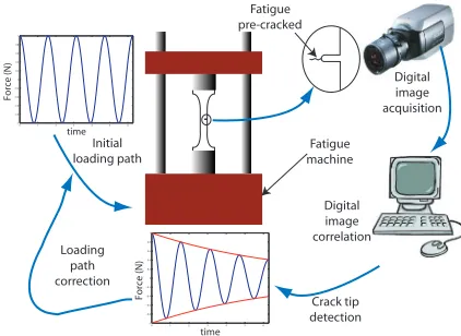
acquisition is driven without stopping the tensile machine thanks to a very short exposition time. The informations given by the Digital Image Correlation procedure (KI or a) are converted into an analogical signal which informs automatically the tensile machine to correct the loading path(figure 3). It is corrected every pre-defined increment of a.
Fatigue machine Fatigue pre-cracked
Digital image correlation
Digital image acquisition
Crack tip detection Loading
path correction
Initial loading path
0 1 2 3 4 5 6 −1
−0.8 −0.6 −0.4 −0.2 0 0.2 0.4 0.6 0.8 1
Force
(N
)
time
0 1 2 3 4 5 6 −1
−0.8 −0.6 −0.4 −0.2 0 0.2 0.4 0.6 0.8 1
For
ce (
N)
time
Fig. 1.Experimental device
4 Fracture parameters identification with Digital Image Correlation
Digital Image Correlation method is based on the optical flow equation (3). The displacement field
Uis searched between a reference digital (grey level) image, f Xand a deformed one,g X.Uis written in a chosen basis function,U X=P
As we want to control the test by using directly DIC, we put the emphasis on the computational cost of the technique. A crude displacement basis is thus elaborated in order to reduce computational cost and perform DIC while the experimental test is running. The displacement is shared into a plane translation, a rotation, an elongation and an discontinuous displacement (equation 4). Because of the notch on the samples and the loading path we know that the crack will propagate along the horizontal direction. A region of interest and a crack direction are defined. Then along the crack direction a dis-continuous basis of function which are commonly used to represent cracks [7], is used: the heavyside function,H(x, y) which is equal to±1 on each side of the crack (equation 5). The crack line is dis-cretized into N nodes.Ni(x) are the linear shape functions which constitute the partition of the unity on those N nodes.
I U = Z Ω h
gX+U− f Xi2dΩ (3)
U=Ut+Ur+Ue+Udis (4)
Udis(x, y)=
N X
i=1
Ui
dis·Φidis(x, y)= N X
i=1
Ui
dis·H(x, y)·Ni(x) (5)
The normal displacement field corresponding to mode I around the crack tip can be expressed into the polar coordinate system (equation 6).
uy=
KI 2µ r r 2πsin θ
2 κ+1−2 cos
2θ
2
(6)
The displacement jump is the difference of it between both sides of the crack (θ=πandθ=−π).
It depends on the square root of the distance to the crack tip r, onKIand the material properties (κand µ) (equation 7).
hh
uy
ii
=uy(r, θ=π)−uy(r, θ=−π)=
KI
µ r r
2π[κ+1] (7)
The square of the jump displacement is linearly interpolated to detect the crack tip (figure 2). The position of the crack is corrected with de rigid motion which is obtained from the calculation ofUt. The stress intensity factorKI is computed with equation 9, P being the slope of the interpolating line. In plane stress, coefficientsκandµare deduced from the Young’s modulus and the Poisson’s ratio at room temperature which are repectively equal to 98GPa and 0.36 for the Zry-4. The Yield stress is equal to 420MPa.
κ= 3−ν
1+ν
µ= 2(1E +ν)
(8)
K1=
µp2·Pπ·lpx
κ+1 (9)
The present method is compared for validation purposes with a more sophisticated decomposition using the Williams’ series formalism as basis function ([8] and [9]). The displacement field in an infinite solid containing a semi-infinite crack is given into polar coordinate with the crack tip as origin. The displacement field is expressed into the complex planu=ux+iuyand can be expressed into the Williams’ series basis decomposition (equation 10) [8].
u=X
n X
k
ωnk·Φnk (10)
0 100 200 300 400 500 600 700 800 0
0.1 0.2 0.3 0.4
Pixel along the crack line
Jump displacement (pixel)
Square of the jump displacement linear interpolation
Fig. 2.Detection of the crack tip and the displacement jump slope using the square of the jump displacement
−9.5 −9 −8.5 −8 −7.5
−10.5 −10 −9.5 −9 −8.5
(a) (b)
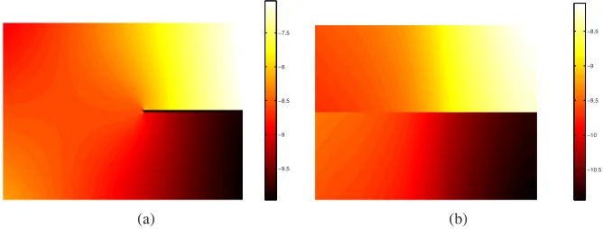
Fig. 3.Normal displacement field using William’s series (Pixels)(a) Normal displacement field using the
simpli-fied basis (Pixels)(b)
different interesting physical meaning. The term corresponding to n=1 gives directly the standard
Westergaard asymptotic displacement field around the crack tip (equation 6). Thus using equation 6, the stress intensity factor can be calculated. The position of the equivalent elastic crack tip is given with n=-1. The crack tip detection is corrected using the rigid motion (n=0).
ΦnI =rn/2
κeinθ/2−n 2e
i(4−n)θ/2+n 2+(−1)
ne−inθ/2 (11)
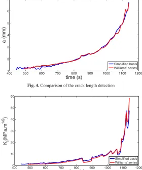
The displacement fields obtained with this two methods ar given on picture 3 (a) and (b). It is notified that the crack tip is represented with more accuracy on the map given with the Williams’ series basis function. However the displacement jump is obtained of the same magnitude. The comparison in the calculation of the crack length and of the stress intensity factor is given into pictures 4 and 5. It shows that the fast detection method is very accurate and can be used as an efficient tool in identifying
4001 500 600 700 800 900 1000 1100 1200 2
3 4 5 6 7
time (s)
a (mm)
Simplified basis Williams’ series
Fig. 4.Comparison of the crack length detection
4000 500 600 700 800 900 1000 1100 1200 10
20 30 40 50 60
time (s)
K I
(MPa.m
1/2
)
Simplified basis Williams’ series
Fig. 5.Comparison of the SIFs estimation
5 Crack propagation control : results
Notched Samples are tested under fatigue cyclic load. The loading rate remains constant and equal to 0.1. A test was driven under a constant maximum force (Fmax) until the complete failure of the sample. A second test was driven with a correction of the maximum force while a is increasing. The width of the sample (W) is equal to 8mm, the thickness (e) is equal to 2.5mm and the notched is about 0.5mm. The loading path is changed every 0.5mm of propagation following equation 12.
Fmax(a)=
σy
2 ·e·(W−a) (12)
The difference between the crack velocity is very strong. In the two cases the crack initiates
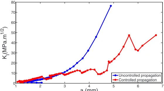
ap-proximatively at the same time but in the second case it is two time faster (picture 6 and 7). Picture 7 shows that with the load shedding method and using this kind of instruction,KIincreases very slowly unless at the end of the failure when boundary effects become predominant. Picture 8 shows that until
a=3mm the difference between the stress intensity factors remains approximatively nil before
increas-ing largely after this value
4001 500 600 700 800 900 1000 1100 1200 2
3 4 5 6 7
time (s)
a (mm)
Uncontrolled propagation Controlled propagation
Fig. 6.Comparison between a load shedding test and constant loading path test on the crack length detection
4000 500 600 700 800 900 1000 1100 1200 10
20 30 40 50 60 70 80
time (s)
K I
(MPa.m
1/2
)
Uncontrolled propagation Controlled propagation
Fig. 7.Comparison between a load shedding test and constant loading path test on the stress intensity factor
estimation
1 2 3 4 5 6 7
0 10 20 30 40 50 60 70 80
a (mm)
K I
(MPa.m
1/2
)
Uncontrolled propagation Controlled propagation
Fig. 8.Comparison of SIF estimation versus the crack length between a load shedding test and constant loading
∆K=∆K0·exp[−C(a−a0)] (13)
∆Kand∆K0are respectively the current and the initial amplitude ofKI.aanda0are respectively the current and the initial crack length. C is a constant relative gradient parameters and it is adviced to be taken as inferior to 0.08mm−1. This kind of correction need a perfect synchronization between the loading force and the image acquisition.
6 Conclusion and perspectives
This method enables us to assist the crack propagation by controlling the loading path. The calculation for one picture, takes less than one second which is largely sufficient in the case of fatigue crack
propagation. The method has the main advantage to produce a pre-crack sample in an all automatic way using a no-contact measurement. By reducing the load during the propagation, the size of fracture plastic zone is limited. Different kind of control will be tested to study the effect on the damage of
the crack propagation. Although a crude basis is used, this method shows a good accuracy when it is compared to a more sophisticated identification basis. A perspective of this work is to confront the accuracy onto the DC potential drop techniques.
References
1. C. E. de Normalisation, Protection contre la corrosion : Terminologie essais de corrosion et pro-tection cathodique Volume 1, AFNOR CEFRACOR, 1999.
2. A. Standard, E647-95, in “1995 ASTM Annual Book of Standards,”, Vol 3 578. 3. C. Bathias, A. Pineau, La fatigue des mat´eriaux et des structures, Maloine, 1980.
4. T. Xu, R. Bea, Load shedding of fatigue fracture in ship structures, Marine Structures 10 (1) (1997) 49–80.
5. S. Roux, J. R´ethor´e, F. Hild, Digital image correlation and fracture, Journal of Physics D: Applied Physics 42 (2009) 214004.
6. I. Hwang, A multi-frequency AC potential drop technique for the detection of small cracks, Mea-surement Science and Technology 3 (1992) 62–74.
7. J. Rethore, S. Roux, F. Hild, From pictures to extended finite elements: Extended digital image correlation (X-DIC), Comptes rendus-M´ecanique 335 (3) (2007) 131–137.
8. S. Roux, F. Hild, Stress intensity factor measurement from digital image correlation: post-processing and integrated approaches, International Journal of Fracture 140 (1-4) (2006) 141–157. 9. M. Williams, On the stress distribution at the base of a stationary crack, ASME Journal of Applied
Mechanics 24 (1957) 109–114.