ABSTRACT
CORNEJO, LUKE R. Multilevel Methods with Multiple Grids in Energy For Multigroup Eigenvalue Transport Problems. (Under the direction of Dmitriy Y. Anistratov).
©Copyright 2019 by Luke R. Cornejo
Multilevel Methods with Multiple Grids in Energy For Multigroup Eigenvalue Transport Problems
by Luke R. Cornejo
A dissertation submitted to the Graduate Faculty of North Carolina State University
in partial fulfillment of the requirements for the Degree of
Doctor of Philosophy
Nuclear Engineering
Raleigh, North Carolina
2019
APPROVED BY:
Yousry Y. Azmy Robin P. Gardner
Carl T. Kelley Dmitriy Y. Anistratov
DEDICATION
BIOGRAPHY
ACKNOWLEDGEMENTS
I want to thank my advisor, Dr. Dmitriy Y. Anistratov, for his years of teaching and guidance in my academic and professional careers. I would also like to thank the faculty of the nuclear engineering department at North Carolina State University who instructed me in both my undergraduate and graduate education. I would especially like to thank Yousry Y. Azmy, Robin P. Gardner, and Carl T. Kelley for being part of my committee and helping direct me in my research.
I extend thanks to Bradley Rearden who provided me with my first national lab experience at Oak Ridge National Laboratory and Jae Chang for my experience at Los Alamos National Laboratory.
TABLE OF CONTENTS
LIST OF TABLES . . . vii
LIST OF FIGURES . . . .viii
Chapter 1 Introduction . . . 1
1.1 Transport Problems . . . 1
1.1.1 QD Method . . . 3
1.1.2 NDA Method . . . 4
1.1.3 pCMFD Method . . . 6
1.2 Diffusion Problems . . . 7
1.3 Multigrid Methods . . . 9
1.4 Significance and Novelty of the Main Results . . . 9
Chapter 2 Multilevel Diffusion Method . . . 12
2.1 Hierarchy of Diffusion Equations . . . 12
2.2 Multigrid Cycles . . . 18
2.3 Prolongation Operators . . . 20
2.3.1 Prolongation with Recursive Correction . . . 20
2.3.2 Prolongation Operator with Constant Approximation in Energy . . . 21
2.3.3 Prolongation Operator with Linear Approximation in Energy . . . 22
2.3.4 Prolongation Operator with Linear Approximation and Factorization . . . 24
2.4 Numerical Results . . . 25
2.4.1 Definition of Tests . . . 25
2.4.2 Analysis of Results on Hierarchies of Nested Grids in Energy . . . 28
2.4.3 Analysis of Results on Hierarchies of Grids with Agglomeration . . . 36
2.5 Summary . . . 38
Chapter 3 Multilevel Transport Method with Multigrid in Energy . . . 40
3.1 Formulation of the Multigroup Low-Order NDA Equations . . . 41
3.2 Formulation of the Multigroup Low-Order Quasidiffusion Equations . . . 43
3.3 The Hierarchy of Low-Order Equations on Multiple Grids in Energy . . . 46
3.4 Multigrid Algorithm . . . 47
3.5 Numerical Results . . . 52
3.5.1 Analysis of Results with Multilevel QD Algorithms with Multigrid in Energy . . . 55
3.5.2 Analysis of Results with Multilevel NDA Algorithms with Multigrid in Energy . . . 60
3.5.3 Analysis of Results with Hybrid Cycle with MLQD . . . 68
3.6 Coarse Grid Multilevel NDA and QD . . . 69
3.6.1 Analysis of Results with Coarse Grid MLNDA . . . 71
3.6.2 Analysis of Results with Coarse Grid MLQD . . . 73
Chapter 4 Multilevel Transport Method with Multigrid in Space and Energy 76
4.1 Formulation of the Low-order CMFD Equations . . . 76
4.2 Formulation of the Low-order CMQD Equations . . . 78
4.3 Formulation of the Low-order Partial Current Based CMFD Equations . . . 80
4.4 Hierarchy of Equations and Multigrid Algorithms . . . 82
4.5 Numerical Results . . . 83
4.5.1 Analysis of Multilevel CMFD . . . 83
4.5.2 Analysis of Multilevel CMQD . . . 86
4.5.3 Analysis of Multilevel pCMFD . . . 88
4.6 Summary . . . 90
Chapter 5 Conclusions. . . 91
5.1 Continuing Lines of Investigation . . . 92
LIST OF TABLES
Table 2.1 Isotope composition of UO2 fuel and number densities [1024cm−3]. . . 25
Table 2.2 Isotope composition of MOX fuel and number densities [1024 cm−3]. . . 25
Table 2.3 Boundaries of energy intervalsEgin eV of the 44-group data library of SCALE 6.1. . . 30
Table 2.4 Boundaries of energy intervals Eg in eV of the 22-group energy grid ΛE,22. . . 30
Table 2.5 Boundaries of energy intervalsEg in eV of the nested energy grids ΛE,8, ΛE,4, and ΛE,2. . . 30
Table 2.6 Test A results on nested grids. . . 31
Table 2.7 Test B results on nested grids. . . 31
Table 2.8 Hierarchies of grids with agglomeration and corresponding sets of nested grids. 38 Table 2.9 Test A results on grids with agglomeration. . . 38
Table 2.10 Test B results on grids with agglomeration. . . 38
Table 3.1 Test A with 44 Group Cross Sections using MLQD with various prolongations. 56 Table 3.2 Test C with 44 Group Cross Sections using MLQD with various prolongations. 57 Table 3.3 Test A with 44 Group Cross Sections using MLNDA with various prolongations. 61 Table 3.4 Test C with 44 Group Cross Sections using MLNDA with various prolongations. 62 Table 3.5 Test A with 44 Group Cross Sections using MLNDA with various RHS calcu-lations. . . 63
Table 3.6 Test C with 44 Group Cross Sections using MLNDA with various RHS calcu-lations. . . 63
Table 3.7 Results with 238 Group Cross Sections using MLNDA. . . 66
Table 3.8 Comparison of Test A using MLNDA based algorithms . . . 67
Table 3.9 Comparison of Test C using MLNDA based algorithms . . . 67
Table 3.10 Hybrid Cycles with 44 Group Cross Sections using MLQD based algorithms. 68 Table 3.11 Results with 44 Group Cross Sections using MLNDA . . . 72
Table 3.12 Boundaries of energy intervalsEg in eV of the 33-group grid. . . 73
Table 3.13 Boundaries of energy intervalsEg in eV of the 26-group energy grid ΛE,26. . . 73
Table 3.14 Boundaries of energy intervalsEg in eV of the 24-group energy grid ΛE,24. . . 73
Table 3.15 Boundaries of energy intervalsEg in eV of the 23-group energy grid ΛE,23. . . 73
Table 3.16 Boundaries of energy intervalsEg in eV of the nested energy grid ΛE,5. . . . 73
Table 3.17 Results with 44 Groups using MLNDA with agglomeration. . . 74
Table 3.18 Results with 44 Group Cross Sections using MLQD . . . 74
Table 3.19 Test A with 44 Group Cross Sections using MLQD . . . 74
Table 4.1 Test A with 44 Group Cross Sections using multilevel CMFD. . . 84
Table 4.2 Test B with 44 Group Cross Sections using multilevel CMFD. . . 85
Table 4.3 Test A with 44 Group Cross Sections using multilevel CMQD. . . 86
Table 4.4 Test B with 44 Group Cross Sections using multilevel CMQD. . . 87
Table 4.5 Test A with 44 Group Cross Sections using multilevel pCMFD. . . 88
LIST OF FIGURES
Figure 2.1 Multigrid cycles for the hierarchies of grids with Γ=2,...,4.GS- Gauss-Seidel iteration over groups on ΛγE, H - homogenization over energy, N - Newton
iteration,P - prolongation . . . 20
Figure 2.2 Geometry and configuration of test problem A. . . 26
Figure 2.3 Geometry and configuration of test problem B. . . 27
Figure 2.4 Pin-cell grid. . . 27
Figure 2.5 The 44-group neutron cross section data generated with SCALE 6.1 data library [66]. . . 28
Figure 2.6 log(Σs,g→g0) . . . 28
Figure 2.7 Measure of strength of group connection, ˜Rg,g0. . . 29
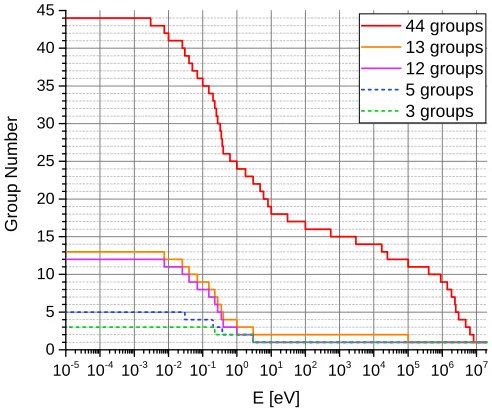
Figure 2.8 The structure of nested energy grids based on the 44-group data library. . . . 32
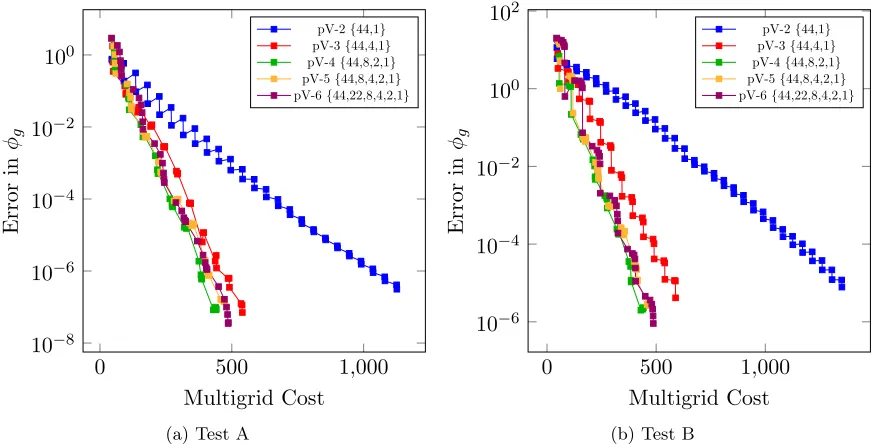
Figure 2.9 Evolution of the ∞-norm of the error for pV-Γ with Iceγ←γ+1 on hierarchies of grids with different number of levels. . . 33
Figure 2.10 Evolution of the ∞-norm of the error for pV-3 with Iceγ←γ+1 on different hierarchies of grids. . . 33
Figure 2.11 Evolution of the ∞-norm of the error for pV-4 with Iceγ←γ+1 on different hierarchies of grids. . . 34
Figure 2.12 Evolution of the ∞-norm of the error for pV-5 with Iceγ←γ+1 on different hierarchies of grids. . . 34
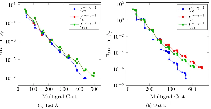
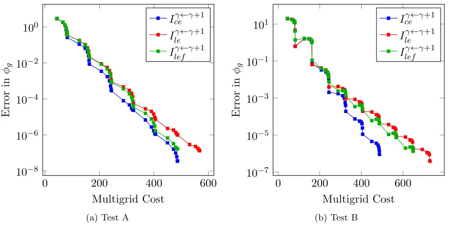
Figure 2.13 Evolution of the ∞-norm of the error for pV-4 withIceγ←γ+1 and Ileγ←γ+1 on the hierarchy of grids{44,8,2,1}. . . 35
Figure 2.14 Evolution of the ∞-norm of the error for pV-5 withIceγ←γ+1 and Ileγ←γ+1 on the hierarchy of grids{44,8,4,2,1}. . . 35
Figure 2.15 Evolution of the ∞-norm of the error for pV-6 withIceγ←γ+1 and Ileγ←γ+1 on the hierarchy of grids{44,22,8,4,2,1}. . . 36
Figure 2.16 The structure of energy grids with agglomeration based on 44-group library. . 37
Figure 3.1 Multigrid pV cycles for grids with Γ = 2−4.GS- Gauss-Seidel iteration over groups on ΛγE,R- projection over angle,H - homogenization over energy,N - Newton iteration,P - prolongation . . . 52
Figure 3.2 Multigrid pW cycles for grids with Γ = 3. GS - Gauss-Seidel iteration over groups on ΛγE,R- projection over angle,H - homogenization over energy,N - Newton iteration,P - prolongation . . . 53
Figure 3.3 Test C geometry and configuration. . . 54
Figure 3.4 Convergence histories of transport iterations of the MLQD method with pV-cycles on hierarchies of grids with different number of levels and constant energy prolongation. . . 58
Figure 3.5 Convergence histories of transport iterations of the MLQD method with pW-cycles on hierarchies of grids with different number of levels and constant energy prolongation. . . 59
Figure 3.7 Convergence histories of transport iterations of the MLNDA method with pV-2 cycle on {44,1} with different right hand sides. . . 64 Figure 3.8 Convergence histories of transport iterations of the MLNDA method with
pV-4 cycle on {44,8,2,1} with different right hand sides. . . 64 Figure 3.9 Convergence histories of transport iterations of the MLQD method on
hier-archies of grids with different number of levels. . . 69 Figure 3.10 Multigrid pV-3 cycle with coarse energy grids. GS - Gauss-Seidel iteration
over groups on ΩγE,R- projection over angle,H- homogenization over energy,
N- Newton iteration,P - prolongation . . . 70
Figure 4.1 Multigrid pV-3 cycle with coarse mesh. GS - Gauss-Seidel iteration over groups on ΩγE,R - projection over angle,M - projection over space, H- ho-mogenization over energy, N- Newton iteration, P - prolongation in energy,
Chapter 1
Introduction
Particles transport processes play important role in various physical phenomena. For a wide class of problems, the basis for mathematical modeling of particle interactions with matter in a physical system is the linear Boltzmann equation [76]. Its solution is the particle distribution function in the phase space and time which enables to determine various characteristics of particle population and predict behavior of the physical system. The physics of nuclear reactors is dominated by the neutron transport and neutron-nuclide interactions. To design and analyze a nuclear reactor it is necessary to model dynamics of neutron population. A particular question about performance of the nuclear system is to determine physical conditions under which there is balance between neutron production and loss. These conditions can be found by solving a certain type of eigenvalue problem for the steady-state Boltzmann equation.
1.1
Transport Problems
To perform nuclear reactor design calculations the multigroup eigenvalue neutron transport problem must be solved. Solving this problem is important for finding the distribution of neu-trons in the reactor and the critical parameter of the system. Current nuclear engineering calculations require the solution of these problems on fine grids in space, angle, and energy. De-sign processes, like coupled multi-physics problems, require the transport problem to be solved many times so it is important to be able to solve these problems quickly.
In order to solve the transport equations they are discretized in to a large system of linear equations. Let us consider the energy grid ΛE withGintervals
Emin =EG < . . . < Eg+1 < Eg < Eg−1< . . . < E0=Emax. (1.1)
by the interval of energy [Eg, Eg−1]. The transport equations with isotropic scattering are
Ω·∇ψg(r,Ω) + Σt,g(r)ψg(r,Ω) =
1 4π
G
X
g0=1
Σs,g0→g(r)
Z
4π
ψg0(r,Ω)dΩ
+ χg(r) 4πk
G
X
g0=1
νf,g0(r)Σf,g0(r)
Z
4π
ψg0(r,Ω)dΩ,r∈G , (1.2a)
ψg(r,Ω)|r∈∂Dvac = 0 and
ψg(r,Ω)|r∈∂Dref =ψg(r,Ω∗)|r∈∂Dref for n·Ω<0, (1.2b)
Ω∗·n=−Ω·n, n·Ω×Ω∗= 0, (1.2c)
g= 1, . . . , G ,
Here
ψg(r,Ω) =
Z Eg−1 Eg
ψ(r,Ω, E)dE (1.3)
is the group angular flux;ψ(r,Ω, E) is the neutron angular flux;k is the multiplication factor; Σt,g is the group total cross section; Σf,g is the group fission cross section; νf,g is the number
of neutrons per fission in the group g; χf,g is the fission spectrum; Σs,g0→g is the scattering
cross section from the group g0 to the groupg;Ωis the unit vector in the direction of neutron flight; nis the outward normal at the boundary∂D,∂Dref is the reflective part of the domain
boundary;∂Dvac is the vacuum boundary; ψg is the group angular flux.
Because of the integro-differential nature of the transport problem it must be solved itera-tively. A classical method of power iterations [52] can converge very slowly for problems with upscattering. This is not suitable for most modern large-scale problems so faster converging methods are needed. There exist several approaches for solving the multigroup transport equa-tion with rapidly converging iteraequa-tions. One family of methods is based on the synthetic acceler-ation approach [52]. An example of such a method is the two-grid acceleracceler-ation scheme developed to speed up iterations in fixed-source transport problems with upscattering [7]. This method uses a one-group diffusion problem for the iterative error. The one-group diffusion coefficient and cross sections are defined by means of a special spectral shape function that approximates the Fourier harmonic of the solution converging at the slowest rate. Another way to solve the k-eigenvalue transport problem is to treat it as a generalized eigenvalue problem and apply Nonlinear Krylov acceleration and Jacobian-Free Newton-Krylov methods [9, 26, 53, 31]. The iterative methods developed on such basis demonstrated efficiency of this approach. Multigrid in energy have also been used as a preconditioner for Krylov solvers [58].
method-ology and effectively reduces the dimensionality of the transport problem [52, 15]. These meth-ods solve a system of equations that consist of the transport equation and a set of lower dimen-sion equations. The low-order equations reduce the dimendimen-sionality of the problem and can form rapidly converging iterative methods. The set of equations is closed by defining linear-fractional factors. These factors are weakly dependent on the high-order which results in accelerated con-vergence. Over the years the NPI methods have seen wide spread used to solve multigroup neutron transport problems.
The detailed formulation of real neutron transport problems involves a very large number of energy groups. For example, the reactor-physics software SCALE for lattice physics calculations uses the 44-group and 238-group ENDF/B-V neutron cross section libraries [66]. The lattice-physics code CASMO-5 for modeling light-water reactors has the 586-group neutron library based on ENDF/B-VII nuclear data [41]. This motivates the development of iteration methods with multiple grids in energy to achieve even better efficiency for full-scale reactor-physics problems.
1.1.1 QD Method
An early NPI method is the Quasidiffusion (QD) method [52, 69, 18, 19]. The set of equations for the QD method consists of the high-order transport equations
Ω·∇ψg(r,Ω) + Σt,g(r)ψg(r,Ω) =
1 4π
G
X
g0=1
Σs,g0→g(r)φg0(r)
+χg(r) 4πk
G
X
g0=1
νf,g0(r)Σf,g0(r)φg0(r),r∈G , (1.4)
and the low-order QD (LOQD) equations [69, 70, 18]. The low-order QD (LOQD) equations for this method are the zeroth and first moments of the transport equation. The set of equations are closed by a set of functionals that are calculated from the high-order solution. If the functionals are exact the LOQD equations can generate the transport solution exactly. The multigroup LOQD equations in continuous form [69, 18, 19] are
∇·Jg+ Σt,gφg= G
X
g0=1
Σs,g0→gφg0+
χg
k
G
X
g0=1
νf,g0Σf,g0φg0, (1.5a)
∇·Egφg
where
Eαβ,g =
R
4πΩαΩβψgdΩ
R
4πψgdΩ
, α, β=x, y (1.6)
are the components of the QD (aka Eddington) tensorEg that is defined to close the system of
high-order transport (1.4) and LOQD equations (1.5). The boundary conditions for the LOQD equations are the following:
n·Jg|r∈∂Gref = 0, n·Jg|r∈∂Gvac =Cn,gφg|r∈∂Gvac, (1.7) where the boundary factor is defined as
Cn,g =
R
Ω·n≥0n·ΩψgdΩ
R
Ω·n≥0ψgdΩ
r
∈∂Gvac
. (1.8)
Reducing the dimensionality of the low-order problem can also be done by using coarser energy grids [69]. Methods with two energy grids, namely involving one-group (grey) low-order problems, were developed based on the Quasi-diffusion method [18, 19, 70, 71, 20, 72, 13, 24]. In the multilevel iteration scheme, the eigenvalue is determined as the solution of the problem with the smallest dimensionality, namely, of the effective one-group low-order equations. This multilevel method can be interpreted as a nonlinear multigrid method and described in terms of projection and prolongation operators. These methods demonstrated that the one-group low-order equation could accelerate the solution of the multigroup low-low-order equation reducing the total amount of work done in the low-order problem.
1.1.2 NDA Method
The Nonlinear Diffusion Acceleration (NDA) method is a very popular NPI method [38]. The low-order equations consist of the zeroth moment of the transport equation and the first moment in the form of a modified Fick’s law equation. The NDA method is similar to the Coarse Mesh Finite Difference (CMFD) [36]. The low-order NDA equations are discretized on the same spatial mesh as the transport equations [36]. The NDA method was originally derived in descrete form [38], but the can also be written continuously [17]. The system of low-order NDA (LONDA) equations in continuous form for the multigroup transport problem (1.2) consists of the neutron balance equation
∇·Jg+ Σt,gφg= G
X
g0=1
Σs,g0→gφg0+ χg
k
G
X
g0=1
and the first-moment equation in the form of the generalized Fick’s law
Jg =−Dg∇φg+ ˜Dgφg, (1.9b)
where
Dg=
1 3Σt,g
, (1.9c)
Jg =
Z
4π
ΩψgdΩ, (1.9d)
is the neutron current and factor ˜Dg is defined to yield exact closure and given by
˜
Dα,g=
R
4πeα·ΩψgdΩ+Dgeα·∇
R
4πψgdΩ
R
4πψgdΩ
, α=x, y . (1.9e) The boundary conditions for the low-order equations are
n·Jg|r∈∂Gvac = Fn,gφg|r∈∂Gvac , Fn=
R
Ω·n≥0
n·ΩψgdΩ
R
Ω·n≥0
ψgdΩ
r∈∂Gvac
, (1.10a)
n·Jg|r∈∂G
ref = 0. (1.10b)
This methodology has been used to accelerate transport methods like the method of character-istics (MOC) [73] and finite element methods [63, 62] and recent work has been done to apply these methods to more types of problems like hexagonal geometries [57].
equations was implemented in the MPACT code [6]. The coarsest energy grid was defined as the two-group problem and the eigen problem was solved on this grid using shifted power iterations. Both pre- and post-sweeps are performed on each multigrid cycle.
1.1.3 pCMFD Method
The classical CMFD method has a zone of instability for certain problems with optically thick meshes in the case the system of the high-order transport equation and low-order CMFD equations is solved using a fixed-point iteration method [25, 34]. A version of CMFD, known as the partial current-based CMFD (p-CMFD) method, has been developed that formulates the low-order problem to preserve the high-order partial currents [55, 35, 54, 64]. It was shown that fixed-point iteration scheme for pCMFD system of equations has better stability properties compared to classical CMFD [55, 61]. The pCMFD equations are usually derived in discrete form. In this section we present a formulation of the pCMFD equations in continuous form. The low-order system of pCMFD equations consists of the zeroth-moment equation
∇ ·Jg+ Σt,gφg= G
X
g0=1
Σs,g0→gφg0+ χg
k
G
X
g0=1
νf,g0Σf,g0φg0 (1.11)
and first-moment equations in the form of a generalized Fick’s law. To derive the pCMFD first-moment equations, we apply theP1 approximation of the angular flux
ψg =
1
4π(φg−3DgΩ·∇φg). (1.12)
Integrating Eq. (1.12) with the weighteα·Ωover 2π±relative to the direction ofeα we get the
P1-approximation for the projection of the partial currents on the directioneα
Jα±= 1 4φg∓
1
2Dgeα·∇φg. (1.13)
We now generalize Eq. (1.13) in the following form:
Jα±=±D˜α,g± φg∓
1
2Dgeα·∇φg. (1.14)
Here we introduced factors ˜D±α,gthat enable one to formulate the exact closure relations for the low-order pCMFD equations. ˜Dα,g± are defined such that
Z
2π±
eα·ΩψgdΩ=±D˜±α,g
Z
4π
ψgdΩ∓
1
2Dgeα·∇
Z
4π
This leads to the factors defined as
˜
Dα,g± = ±
R
2π±eα·ΩψgdΩ∓12Dgeα·∇
R
4πψgdΩ
R
4πψgdΩ
. (1.16)
We now take into account that α-component of the current eα·Jg is given by
Jα,g =Jα,g+ −Jα,g− (1.17)
to obtain the pCMFD form of the generalized Fick’s law
Jα,g=−Dgeα·∇φg+ ( ˜D−g + ˜D+g)φg. (1.18)
Thus the low-order pCMFD equations are given by Eqs. (1.11) and (1.18). The boundary conditions for the low-order equations are defined in (1.10). Fourier analysis of pCMFD method with Step Characteristics for 1-dimensional eigenvalue problems is unconditionally stable [61]. The pCMFD method has been applied to accelerate the step characteristics method in NEWT [35]. It has also be used as an accelerator in whole-core transport solutions [64, 5].
1.2
Diffusion Problems
The phase space of neutron transport problems has high dimensionality. It includes the spatial position of the particle, its energy and the direction of particle motion. In general case, it is a 6-dimensional space. To reduce the dimensionality of the problem and complexity of neutron transport simulations, various approximate methods have been developed. One group of neutron transport models is based on the P1 equations that belong to the family of the method of spherical harmonics also know as the PN method [16]. The P1 equations are defined for the first two moments of the neutron angular flux and hence of the distribution function. The moment equations are closed assuming that the angular flux linearly depends on the direction of particle motion. The P1 equations can be reduced to the neutron diffusion equation for the zeroth angular moment of the angular flux.
ΛE is defined by [16]
−∇·Dg(r)∇φg(r) + Σt,g(r)φg(r) = G
X
g0=1
Σs,g0→g,(r)φg0(r)
+χg(r)
k
G
X
g0=1
νf,g0(r)Σf,g0(r)φg0(r), (1.19) r∈ D, g= 1, . . . , G ,
with the following conditions
n(rb)·∇φg(rb) = 0, rb ∈∂Dref (1.20)
at the reflective boundary and
φg(rb) + 2Dg(rb)n(rb)·∇φg(rb) = 0, rb ∈∂Dvac (1.21)
at the vacuum boundary. Dg = 3Σ1t,g is the group diffusion coefficient; n(rb) is the outward
normal at the boundary. The P1 equations are given by the neutron balance equation
∇·Jg(r) + Σt,g(r)φg(r) = G
X
g0=1
Σs,g0→g,(r)φg0(r) +χg(r)
k
G
X
g0=1
νf,g0(r)Σf,g0(r)φg0(r) (1.22)
and the Fick’s law
Dg(r)∇φg(r) +Jg(r) = 0. (1.23)
The solution of the P1 equations has limited accuracy. However, it works well for neutron transport problems in which the angular flux weakly depends on angular and spatial variables. The diffusion solution is a good approximation for problems that involve spatial homogenization [47, 65]. A lot of research has been carried out to study properties and applicability of the P1 method and diffusion approximation [46, 23, 22, 48, 28]. The P1 method is a reliable tool for modeling and analysis of various of physical systems [37, 11].
applied to develop a nonlinear two-grid (NTG) method for multigroup diffusion problems [14]. The stability properties of the NTG method for k-eigenvalue multigroup diffusion problems has been studied by means of the Fourier analysis. This analysis predicted well the rates of convergence of the eigenvalue and associated eigenfunction.
1.3
Multigrid Methods
Multigrid methods were originally developed for solving boundary value problems found in may physical systems[59, 60, 75]. A linear system of equations is formed from the elliptic partial differential equations by finite element or finite difference discretization. For this type of system of equations local relaxations, such as Gauss-Seidel and Jacobi iterations, converge very fast on the high frequency part of the solution. The low frequency component of the solution can converge much slower. The convergence of the iterative method can be improved by introducing a coarser grid and projecting the error onto it. The first effect of this is to reduce the size of the problem. The second is that the slow to converge low frequency error effectively becomes a higher frequency error on the coarser grid and can be efficiently corrected by local relaxations on that grid. Repeating this recursively yields a multigrid iterative method. The set of nested coarse grids are found by successive refinement. These types of methods are known as geometric multigrid as they are dependent on a hierarchy of geometric grids.
Algebraic multigrid is a generalization of geometric multigrid [39, 32]. It was originally developed for sets of equations similar to discretized PDEs approximated on an unstructured grid. This methodology has been extended to other types of problems and general matrices.
Multigrid method can be applied to solve neutron transport problems. Spatial multigrid methods have been developed to accelerate transport problems and be well suited for parallel computation [4]. A multilevel in space and energy method for diffusion problems has been developed that uses geometric multigrid in space linear solver [2, 3]. This method also uses two levels in energy. Multigrid has also been used as a preconditioner for solving transport problems [58].
1.4
Significance and Novelty of the Main Results
transport methods for reactor-physics application are proposed based on low-order equations of the QD, NDA, CMFD, and pCMFD methods.
We defined several variants of prolongation operators based on multiplication correction of the grid solutions. The prolongation operators use constant and linear interpolation in energy between neighboring grids. We apply the partial V-cycles, partial W-cycles, and hybrid cycles to move through the hierarchy of energy grids. The estimation of the eigenvalue is performed on the coarsest grid with just one energy group. Thus, the eigenvalue problem is solved in the space with the smallest dimensionality. The proposed methods with multigrid in energy are derived for the second-order finite volume spatial discretization of the low-order transport (and diffu-sion) equation. They can be applied to other spatial discretizations as well, for example, finite element methods. The obtained numerical results on realistic model reactor-physics problems with 44 and 258 groups demonstrated efficiency of the developed algorithms with multigrid in energy. They enable to reduce significantly total number of low-order solves as well as accelerate transport iterations. Involving additional coarse energy grids accelerate iterations and decrease computational costs.
The proposed multilevel methods enable one to solve important class reactor physics prob-lem. They are effective in solving the large-scale transport problems and can be used, for instance, for full-core like calculations. These methods can be applied to different transport methods to improve performance of existing reactor-physics software. The proposed multilevel algorithms can be used to develop advanced iterative methods for solving large-scale multi-physics problems with very large number of groups.
This research was presented by the candidate to members of the research community at the following venues:
Joint International Conference on Math and Computation (M&C), Supercomputers in Nuclear Applications (SNA) and the Monte Carlo (MC) Method in Nashville, TN, April 19-23, 2015
The Physics of Reactors (PHYSOR) Conference in Sun Valley, ID, May 1-5, 2016
Scientific Seminar to Laboratory, Reactor and Nuclear Systems Division at Oak Ridge National in Oak Ridge, TN, July 30, 2018, and
Scientific Seminar to Radiation Transport Group at Los Alamos National Laboratory in Los Alamos, NM, August 22, 2018,
Chapter 2
Multilevel Diffusion Method
In this chapter we present a nonlinear method with multiple grids in energy for solving the k-eigenvalue problem for multigroup neutron diffusion equations. We develop multigrid-in-energy algorithms based on a nonlinear projection operator and several prolongation operators. The evaluation of the eigenvalue is performed in the space with smallest dimensionality by solving the effective one-group diffusion problem. The multilevel methods are formulated in discrete form for the second-order finite volume discretization of the diffusion equation. The homogenization in energy is based on a spatially consistent discretization of the group diffusion equations on coarse grids in energy. The results of this chapter has been submitted for publication [40].
In Sec. 2.1 the hierarchy of equations is defined. Sec. 2.2 describes the multigrid cycles and Sec. 2.3 defines the prolongation operators. Numerical results are presented in Sec. 2.4.
2.1
Hierarchy of Diffusion Equations
To formulate the multilevel method for solving Eq. (1.19) we define a hierarchy of grids in energy [44, 45]
{ΛγE, γ= 1, . . . ,Γ : ΛΓE ⊂. . .⊂ΛγE ⊂ΛγE−1 ⊂. . .⊂Λ1E = ΛE}, (2.1)
whereγ is the grid index. The grid ΛγE consists of groups with energy intervalsδEgγ = [Egγ, Egγ−1] (g = 1, . . . , Gγ) formed by coarsening the previous grid ΛγE−1. Gγ is the number of groups in the grid ΛγE. Thus, the group scalar flux on the grid ΛγE is given by
φγp =
Z
δEgγ
φ(r, E)dE= X
g0∈ωγ p
where ωpγ is the set of group indices of the grid ΛγE−1 included in the groupg of the grid ΛγE.
The grid Λ1E is the given fine energy grid. ThusG1 =Gand
φg(r)≡φ1g(r). (2.3)
The coarsest grid ΛΓE has only one group andGΓ= 1. The total scalar flux is given by
φ(r) =
Z Emax Emin
φ(r, E)dE=φΓ1(r). (2.4)
The methods with multigrid in energy are formulated by means of projection and prolon-gation operators. The nonlinear projection operator is defined by integration of the diffusion equations over energy groups and their homogenization with respect to energy. The homoge-nization procedure transfers information from a grid to a coarser one and defines a coarse-grid correction step. The hierarchy of group diffusion equations on multiple grids in energy has the following general form:
−∇2D¯γp(r)φγp(r)
+ ¯Σγt,g(r)φγp(r) =
Gγ
X
g0=1
¯
Σγs,g0→g(r)φγg0(r) +
¯
χγg(r)
k
Gγ
X
g0=1
νΣγf,g0(r)φγg0(r), (2.5) r∈ D, g= 1, . . . , Gγ, γ = 1, . . . ,Γ−1,
−∇2D¯Γ1φΓ1(r)+ ¯ΣΓa,1φΓ1(r) = 1
kνΣ
Γ
f,1φΓ1, r∈ D, γ = Γ. (2.6)
The cross sections and diffusion tensor ¯Dγp are averaged by the solution φγg−1 on the grid ΛγE−1.
The averaged cross sections are given by
¯ Σγt,g =
P
g0∈ωγ g
¯ Σγt,g−01φ
γ−1
g0
P
g0∈ωγ g φ
γ−1
g0
, Σ¯γa,g =
P
g0∈ωγ g
¯ Σγa,g−10φ
γ−1
g0
P
g0∈ωγ g φ
γ−1
g0
, (2.7a)
νΣγf,g =
P
g0∈ωγ g νΣ
γ−1
f,g0φγg0−1
P
g0∈ωγ g φ
γ−1
g0
, χ¯γg = X
g0∈ωγ g
¯
χγg0−1, (2.7b)
¯
Σγs,g0→g =
P
g0∈ωγ g0
P
g∈ωγp ¯ Σγs,g−01→g
φγg0−1
P
g0∈ωγ g0
φγg0−1
, (2.7c)
where ¯Σ1
t,g = Σt,g, νΣ
1
f,g = νf,gΣf,g, ¯Σ1s,g0→g = Σs,g0→g, ¯D1p = diag(Dp, . . . , Dp). We note
diffusion equations. The continuous equations (2.5) and (2.6) lack some essential details. The diffusion tensor ¯Dγp and the form of the discretized differential term are defined by averaging of
the discrete leakage rate density (LRD) term and depend on the spatial discretization scheme. This part of the methodology is described below.
To solve the group diffusion equations (2.5) on ΛγE withγ <Γ, we evaluate the fission and upscattering terms by means of the solution obtained on the grid ΛγE−1 and use the estimation of the eigenvalue from the previous multigrid cycle. The equation (2.5) gives rise to
−∇2 D¯γgφγg
+ ¯Σγt,gφγg −
g
X
g0=1
¯
Σγs,g0→gφ γ g0 =
Gγ
X
g0=g+1
¯ Σγs,g0→g
X
g0∈ωγ g0
φγg0−1+
¯
χγg
k
Gγ
X
g0=1
νΣγf,g0
X
g0∈ωγ g0
φγg0−1, (2.8)
g= 1, . . . , Gγ
for γ = 1, . . . ,Γ−1. Thus, the equations for φγ = (φγ1, . . . , φγG)T have the following general
form:
Aγφγ =Bγφγ−1+
1
kCγφ
γ−1, (2.9)
whereAγ is operator of the left-hand side of Eq. (2.8) given by
Aγφγ≡ −∇2 D¯γgφγg
+ ¯Σγt,gφγg− g
X
g0=1
¯
Σγs,g0→gφγg0, (2.10) Bγ and Cγ are the upscattering and fission production operators, respectively, defined as
Bγφγ−1 ≡ Gγ
X
g0=g+1
¯ Σγs,g0→g
X
g0∈ωγ g0
φγg0−1, Cγφγ−1 ≡χ¯γg Gγ
X
g0=1
νΣγf,g0
X
g0∈ωγ g0
φγg0−1. (2.11)
The matrix-operator Aγ is lower triangular. The system of group diffusion equation (2.8) on
the grid ΛγE can be solved by sweeping through groups. This is equivalent to performing one Gauss-Seidel iteration over energy groups on this grid.
The eigenvalue and associated one-group eigenfunction are determined by solving the effec-tive one-group problem (2.6). The eigenvalue problem on the coarsest grid ΛΓE has the following general form:
AΓφΓ= 1
kCΓφ
where
AΓφΓ≡ −∇2
¯
DΓ1φΓ1
+ ¯ΣΓa,1φΓ1, CΓφΓ=νΣ Γ
f,1φΓ1 . (2.13)
We consider problems in 2D Cartesian geometry with the rectangular spatial domain D=
{0 ≤ x ≤ X, 0 ≤ y ≤ Y}. The spatial grids are orthogonal and defined by the cells Cij = {xi−1/2 ≤ x ≤ xi+1/2, yj−1/2 ≤ y ≤ yj+1/2}, where i = 1, . . . , Nx, j = 1, . . . , Ny. The cross
sections are assumed to be piece-wise constant functions on the set of grid cells. The group diffusion equations (1.19) on ΛE are approximated by means of a second-order finite volume
(FV) method which is derived by discretizing theP1 equations (1.22) and (1.23). We integrate the balance equation (1.22) over the cell Cij to get
Jg,i+1/2,j−Jg,i−1/2,j
hyj + Jg,i,j+1/2−Jg,i,j−1/2
hxi + Σt,g,i,jφg,i,jAi,j =
Ai,j G
X
g0=1
Σs,g0→g,i,jφg0,i,j+ 1
kAi,jχg,i,j
G
X
g0=1
νf,g0,i,jΣf,g0,i,jφg0,i,j, (2.14)
hxi =xi+1/2−xi−1/2, hyj =yj+1/2−yj−1/2, Ai,j =hxih y
j, (2.15)
where φg,i,j is the cell-average group scalar flux, Jg,i+1/2,j and Jg,i,j+1/2 are the face-average group currents, Σt,g,i,j, Σf,g,i,j,νf,g,i,j, Σs,g0→g,i,j, and χg,i,j are the material parameters of the
cellCij. The Fick’ law (1.23) is integrated over right, left, bottom, and top halves of Cij. This
yields
Dg,i,j φg,i+1/2,j−φg,i,j
+1
2Jg,i+1/2,jh
x
i = 0, (2.16)
Dg,i,j φg,i,j−φg,i−1/2,j
+1
2Jg,i−1/2,jh
x
i = 0, (2.17)
Dg,i,j φg,i,j−φg,i,j−1/2
+1
2Jg,i,j−1/2h
y
j = 0, (2.18)
Dg,i,j φg,i,j+1/2−φg,i,j
+1
2Jg,i,j+1/2h
y
j = 0, (2.19)
where φg,i+1/2,j and φg,i,j+1/2 are the face-average group scalar fluxes, and Dg,i,j = 3Σt,g,i,j1 .
Eliminating the face-average scalar fluxes in Eqs. (2.16)-(2.19), we get the following relations between the face-average currents and cell-average scalar fluxes
Jg,i+1/2,j=−
Dg,i+1/2,j hx
i+1/2
φg,i+1,j−φg,i,j
, (2.20)
Jg,i,j+1/2=−Dg,i,j+1/2
hyj+1/2 φg,i,j+1−φg,i,j
hxi+1/2 = 1 2(h
x
i +hxi+1), h
y j+1/2=
1 2(h
y j +h
y
j+1), (2.22)
where the cell-face diffusion coefficients are given by
Dg,i+1/2,j =
2Dg,i,jDg,i+1,jhxi+1/2
Dg,i,jhxi+1+Dg,i+1,jhxi
, Dg,i,j+1/2 =
2Dg,i,jDg,i,j+1hyj+1/2
Dg,i,jhyj+1+Dg,i,j+1hyj
. (2.23)
Substituting Eqs. (2.20) and (2.21) into the cell-balance equation (2.14), we obtain the dis-cretized group diffusion equations for the cell-average group scalar fluxesφg,i,j on the given fine
grid ΛE of the following form:
−
"
Dg,i+1/2,j hx
i+1/2
φg,i+1,j−φg,i,j
−Dhg,ix−1/2,j i−1/2
φg,i,j−φg,i−1,j
#
hyj
−
"
Dg,i,j+1/2
hyj+1/2 φg,i,j+1−φg,i,j
−Dhg,i,jy −1/2 j−1/2
φg,i,j−φg,i,j−1
#
hxi + Σt,g,i,jφg,i,jAi,j =
Ai,j G
X
g0=1
Σs,g0→g,i,jφg0,i,j+ 1
kAi,jχg,i,j
G
X
g0=1
νf,g0,i,jΣf,g0,i,jφg0,i,j. (2.24)
The first two terms on the left-hand side of Eq. (2.24) define the discrete LRD term of the applied FV scheme.
The discrete group diffusion equations on the grid ΛγE are formulated to be algebraically consistent with the equations on the grid ΛγE−1. The homogenization of the equations over energy intervals is performed without any approximation. To derive the diffusion equations on the hierarchy of grids, we start by formulating discrete equations on Λ2E and sum the equations (2.24) on Λ1E overg-th interval of the grid Λ2E. The LRD term in Eq. (2.24) is summed overωg2
and cast in terms of φ2g,i,j in the following way:
− h y j
hxi+1/2 X
g∈ω2 p
Dg,i+1/2,j φg,i+1,j−φg,i,j
+ h
y j
hxi−1/2 X
g∈ω2 p
Dg,i−1/2,j φg,i,j−φg,i−1,j
− h x i
hyj+1/2 X
g∈ω2 p
Dg,i,j+1/2 φg,i,j+1−φg,i,j
+ h
x i
hyj−1/2 X
g∈ω2 p
Dg,i,j−1/2 φg,i,j −φg,i,j−1=
− h y j
hx i+1/2
¯
Dg,i+,2+1/2,jφ2g,i+1,j−D¯g,i−,2+1/2,jφ2g,i,j+ h
y j
hx i−1/2
¯
Dg,i+,2−1/2,jφ2g,i,j−D¯g,i−,2−1/2,jφ2g,i−1,j
− h x i
hyj+1/2
¯
Dg,i,j+,2+1/2φ2g,i,j+1−D¯g,i,j−,2+1/2φ2g,i,j
+ h
x i
hyj−1/2
¯
D+g,i,j,2−1/2φg,i,j−D¯−g,i,j,2−1/2φg,i,j−1
where we defined the cell-face diffusion coefficients on the grid Λ2
E
¯
D+g,i,2+1/2,j=
P
g∈ω2
gDg,i+1/2,jφg,i+1,j
P
g∈ω2
gφg,i+1,j
, D¯−g,i,2+1/2,j =
P
g∈ω2
gDg,i+1/2,jφg,i,j
P
g∈ω2 gφg,i,j
, (2.26)
¯
D+g,i,j,2+1/2=
P
g∈ω2
gDg,i,j+1/2φg,i,j+1
P
g∈ω2
gφg,i,j+1
, D¯−g,i,j,2+1/2 =
P
g∈ω2
gDg,i,j+1/2φg,i,j
P
g∈ω2 gφg,i,j
. (2.27)
It can be shown by mathematical induction that the general form of the discrete LRD term on any coarse grid ΛγE (γ >1) has the form of the discretized LRD term on Λ2
E. It is given by
Lγg,i,jφ γ g ≡ −
hyj hx
i+1/2 ¯
D+g,i,γ+1/2,jφγg,i+1,j−D¯g,i−,γ+1/2,jφγg,i,j
+ h
y j
hxi−1/2 D¯
+,γ g,i−1/2,jφ
γ
g,i,j−D¯− ,γ g,i−1/2,jφ
γ g,i−1,j
− h x i
hyj+1/2 D¯
+,γ g,i,j+1/2φ
γ
g,i,j+1−D¯−
,γ g,i,j+1/2φ
γ g,i,j + h x i
hyj−1/2
¯
Dg,i,j+,γ−1/2φg,i,j−D¯g,i,j−,γ−1/2φg,i,j−1, (2.28) where cell-face diffusion coefficients on ΛγE are calculated by the solution of the previous grid as follows:
¯
Dg,i+,γ+1/2,j=
P
g0∈ωγ g
¯
Dg+0,γ,i+1−1/2,jφ γ−1
g0,i+1,j
P
g0∈ωγ g φ
γ−1
g0,i+1,j
, D¯−g,i,γ+1/2,j=
P
g0∈ωγ g
¯
Dg−0,γ,i+1−1/2,jφ γ−1
g0,i,j
P
g0∈ωγ g φ
γ−1
g0,i,j
, (2.29a)
¯
Dg,i,j+,γ+1/2=
P
g0∈ωγ g
¯
Dg+0,γ,i,j−+11 /2φ γ−1
g0,i,j+1
P
g0∈ωγ g φ
γ−1
g0,i,j+1
, D¯−g,i,j,γ+1/2=
P
g0∈ωγ g
¯
Dg−0,γ,i,j−+11 /2φ γ−1
g0,i,j
P
g0∈ωγ g φ
γ−1
g0,i,j
, (2.29b)
where
¯
Dg,i+,1+1/2,j = ¯Dg,i−,+11 /2,j =Dg,i+1/2,j D¯g,i,j+,1+1/2= ¯Dg,i,j−,1+1/2 =Dg,i,j+1/2. (2.29c) We note that this homogenization in energy on a coarse energy grid yields two diffusion coeffi-cients at each face.
The final discrete form of the group diffusion equations (2.5) and (2.6) on the hierarchy of grids is the following:
Lγg,i,jφγg + ¯Σ γ t,g,i,jφ
γ
g,i,jAi,j =
Ai,j G
X
g0=1
¯
Σγs,g0→g,i,jφγg0,i,j+
1
kχ¯
γ g,i,jAi,j
G
X
g0=1
g= 1, . . . , Gγ, γ = 1, . . . ,Γ−1,
LΓ1,i,jφΓ1 + ¯Σa,Γ1,i,jφΓ1,i,jAi,j =
1
kAi,jνΣ
Γ
f,1,i,jφΓ1,i,j. (2.31)
The cross sections and other material properties are defined according to Eqs. (2.7a)-(2.7c) by their cell-average values, for example,
¯
Σγt,g,i,j =
P
g0∈ωγ g
¯
Σγt,g−01,i,jφγg0−,i,j1
P
g0∈ωγ g φ
γ−1
g0,i,j
. (2.32)
2.2
Multigrid Cycles
To solve the multilevel system of group diffusion equations (2.30) and (2.31) on the hierarchy of grids in energy, we apply multigrid algorithms with different types of cycles. We use partial V-cycles pV-Γ which are described in Algorithm 1 and shown in Figure 2.1. ThepV-Γ algorithm
φ0 ≡φ1
for γ ←1 toΓ−1do
Solveφγ=A−1
γ Bγφγ−1+
1
kA
−1
γ Cγφγ−1
Perform homogenization in energy to formAγ+1,Bγ+1,Cγ+1
end
Solve the eigenvalue problem CΓ−1AΓφΓ=kφΓ to updatek and φΓ
for γ ←Γ−1 to 1 do
Perform prolongationφγ←Iαγ←γ+1φγ+1 end
Algorithm 1: pV-Γ. The multigrid algorithm with the partial V-cycle.
The pV-Γ algorithm moves from the coarsest grid ΛΓ
E towards the finest grid Λ1E without
solving group diffusion equations on any grid. This is shown on the cycle graphs by open circles. The prolongation procedure between grids uses one of versions of the interpolation operator
Iαγ←γ+1 described in Sec. 2.3. The subscript α indicates the type of interpolation α=ce: the correction factor based on constant approximation in energy,
α=le: the correction factor based on linear approximation in energy,
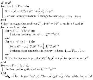
α=lef: the correction factor based on linear approximation in energy with factorization. Figure 2.1 shows various multigrid cycles. The partial V-cycle can be viewed as\-cycle. Another kind of multigrid algorithm uses nested iterations involving coarse grids. It can be interpreted as a partial W-cycle. Algorithm 2 presents thepW-Γ(γ∗, µ) algorithm, where the nested multigrid cycles start from the grid ΛγE∗ and are executedµtimes. Figure 2.1c illustrates the pW-3(2,1)
φ0 ≡φ1
for γ ←1 toΓ−1do
Solveφγ=A−1
γ Bγφγ−1+
1
kA
−1
γ Cγφγ−1
Perform homogenization in energy to formAγ+1,Bγ+1,Cγ+1
end
Solve the eigenvalue problem CΓ−1AΓφΓ=kφΓ to updatek and φΓ
for m←1 to µdo
forγ ←Γ−1 to γ∗ do
Perform prolongationφγ←Iαγ←γ+1φγ+1 end
forγ ←γ∗ to Γ−1 do
Solveφγ =A−1
γ Bγφγ−1+
1
kA
−1
γ Cγφγ−1
Perform homogenization in energy to formAγ+1,Bγ+1,Cγ+1
end
Solve the eigenvalue problemCΓ−1AΓφΓ=kφΓ to updatekand φΓ
end
for γ ←Γ−1 to 1 do
Perform prolongationφγ←Iαγ←γ+1φγ+1 end
Algorithm 2:pW-Γ(γ∗, µ). The multigrid algorithm with the partial W-cycle.
algorithm.
An important characteristic of a multigrid algorithm is the number of cycles (Nc) that it
1 2 GS N H P 𝛾𝛾 1 2 GS NN H P 𝛾𝛾
(a)pV-2
1 2 3 GS GS N H H P 𝛾𝛾 1 2 3 GS GS N H H P 𝛾𝛾 GS N P P P H
(b)pV-3
1 2 3 GS GS N H H P 𝛾𝛾 1 2 3 GS GS N H H P 𝛾𝛾 GS N P P P H
(c)pW-3(2,1)
𝛾𝛾 1 2 3 4 GS GS GS N H H H P P P
(d)pV-4
Figure 2.1: Multigrid cycles for the hierarchies of grids with Γ=2,...,4.GS- Gauss-Seidel itera-tion over groups on ΛγE,H- homogenization over energy,N- Newton iteration,P- prolongation
a cycle. However, the cost of each cycle affects the algorithm efficiency. It varies for different algorithms. The optimum algorithm for a test is the one which requires the minimum total number of diffusion solves (Nds). For the given numbers of cycles and groups in each grids, the
total number of diffusion solves can be calculated as
Nds =Nc
Γ
X
γ=1
Gγ+ 1 (2.33)
for thepV-Γ algorithm and
Nds=Nc
XΓ
γ=1
Gγ+µ
Γ
X
γ=γ∗
Gγ
+ 1 (2.34)
for thepW-Γ(γ∗, µ) algorithm.
2.3
Prolongation Operators
2.3.1 Prolongation with Recursive Correction
We formulate prolongation operators as an interpolation procedure based on a multiplicative correction of the solution. The corrected group scalar flux ˆφγg on the grid ΛγE is defined as
correction factorfγg+10 computed using solutions on two neighbouring energy grids Λ γ E and Λ
γ+1
E
ˆ
φγg(~r) =φgγ(~r)fα,gγ+10(~r), g∈ωgγ0+1. (2.35)
The interpolation procedure performs recursive calculation of factors and solution correction on each grid according to Algorithm 3, where γ∗ = 1 for thepV-Γ cycle. In this algorithm, the correction factor generally depends on the corrected solutions on coarser grids
fγα,g+10 =f γ+1
α,g0
φγ,φˆγ+1, . . . ,φˆΓ−1, φΓ
, (2.36)
and hence on the corresponding factors. Hereafter we refer to this type of operator as the prolongation operator with recursive correction factors (RCF).
for γ ←Γ−1 to γ∗ do
Compute correction factorsfγα,g+10,g0 = 1, . . . , Gγ+1
Perform interpolation on the grid ΛγE : ˆφγg =φgγfγα,g+10,g∈ω γ+1
g0 ,g= 1, . . . , Gγ end
Algorithm 3: Prolongation operatorIαγ←γ+1 with recursive correction factors
2.3.2 Prolongation Operator with Constant Approximation in Energy
The prolongation operators use different definitions of correction factors. The first variant of the prolongation operator is based on a group-local factor associated with the coarse grid ΛγE+1that involves only one energy interval on this grid. It uses constant approximation of the solution over the energy interval δEgγ+1 and is formulated as follows:
fγce,g+1(r) = φˆ
γ+1
g (r)
P
g0∈ωγ g φ
γ g0(r)
, g= 1, . . . , Gγ+1. (2.37) This defines the operatorIceγ←γ+1that is referred to as the prolongation operator with constant
approximation in energy. It can be shown that application of the factor (3.28) recursively ac-cording to Algorithm 3 is equivalent to the following factorization form of the operatorIceγ←γ+1:
ˆ
where
˜fγ+1
ce,g(r) =
φγg+1(r)
P
g0∈ωγ g φ
γ g0(r)
, g= 1, . . . , Gγ+1. (2.39) Thus, the group scalar flux on the grid ΛγE is corrected by the product of the factors (3.30) computed by the solutions on coarser grids from the current multigrid cycle.
2.3.3 Prolongation Operator with Linear Approximation in Energy
We now formulate the correction factor based on the linear approximation in energy using the solution over two energy intervals of ΛγE+1. The scalar flux on the grid ΛγE over intervals g and
g+ 1 of the grid ΛγE+1 approximated by its group-average values can be cast as follows: Φγg,γ+1(r, E) = X
g0∈ωγ+1 g ∪ωγg+1+1
φγg0(r)
∆Egγ0
H(E−Eγg0)−H(E−E γ g0−1)
,
E ∈δEgγ+1+1∪δEgγ+1, (2.40)
∆Egγ0 =Egγ0−1−Egγ0, (2.41)
where H is the Heaviside step function
H(x) =
0 x <0 1
2 x= 0 1 x >0
. (2.42)
The updated scalar flux on the grid ΛγE is defined by the following interpolation function:
ˆ
Φγg←γ+1(r, E) = Φγg,γ+1(r, E)Fgγ+1(r, E) for E ∈δEgγ+1+1∪δEgγ+1, (2.43) where the factorFpγ+1 is the linear function in energy given by
Fgγ+1(E) = ¯FE,gγ+1+ 2
∆Egγ+1+ ∆Egγ+1+1
E−E¯gγ+1
˜
FE,gγ+1, (2.44)
∆Egγ+1=Egγ−+11 −Egγ+1, E¯gγ+1 = 1 2
Egγ−+11 +Egγ+1+1. (2.45) The coefficients ¯FE,gγ+1 and ˜FE,gγ+1 are determined by means of the solution on the grid ΛγE+1 from the following conditions:
Z
δEgγ+1 ˆ Φγ←γ+1
Z
δEgγ+1+1
ˆ
Φγg←γ+1(r, E)dE= ˆφγg+1+1(r). (2.47) The corrected scalar flux ˆΦγg←γ+1(E) is used to update the group scalar fluxes on the grid ΛγE
over just one interval of the grid ΛγE+1. We apply it to correct the solution over the interval
δEgγ+1+1 as follows:
ˆ
φγg0(r) =
Z
δEgγ0
ˆ Φγ←γ+1
g (r, E)dE for g0∈ω γ+1
g+1. (2.48)
This leads to the multiplicative correction of the solution on the grid ΛγE by the solution on the coarser grid ΛγE+1 given by
ˆ
φγg0(r) =φ γ g0(r)f
γ+1
le,g0←g(r), g0∈ω γ+1
g+1, g0= 1, . . . , Gγ, (2.49) where the correction factor fγle,g+10←g is defined as
fγle,g+10←g(r) =
1 ∆Egγ0
Z
δEgγ0
Fgγ+1(r, E)dE . (2.50)
The interpolation procedure (2.49) is applied recursively according to Algorithm 4. This defines the prolongation operatorIleγ←γ+1. Hereafter we referred to it as the prolongation operator with linear approximation in energy.
for γ ←Γ−1 to γ∗ do
Compute correction factorsfγα,g+10←g,g0 = 1, . . . , Gγ,g= 1, . . . , Gγ+1
Perform interpolation on the grid ΛγE : ˆφγg0(r) =φ γ g0(r)f
γ+1
α,g0←g(r) , g0∈ω γ+1
g+1
end
Algorithm 4: Prolongation operatorIleγ←γ+1 with RCF.
The interpolation function (2.43) can also be applied to update group scalar fluxes on the grid ΛγE over the interval δEgγ+1
ˆ
φγg0(r) =
Z
δEgγ0 ˆ
Φγg←γ+1(r, E)dE for g0∈ωgγ+1. (2.51) This mapping is used for g = 1. We note that the coarsest grid ΛΓE has only one interval. To update the solution on ΛΓE−1 we use the group-local factors with constant approximation in energy and hence set
where g = 1. If the slope of the correction is large, the interpolated solution ˆΦγg←γ+1(E) can
be negative for E ∈ δEgγ+1+1∪δE
γ+1
g . If this is the case, then we use the correction factor with
constant approximation in energy and set
fγle,g+10←g(r) =fγce,g+1(r). (2.53)
Other slope-limiting techniques can also be applied to the interpolation factor (2.44) to adjust the slope ˜FE,gγ+1.
2.3.4 Prolongation Operator with Linear Approximation and Factorization
To formulate prolongation operators with non-recursive factors we generalize the factorization form of the operator Iceγ←γ+1 and define interpolation with linear approximation as a product
of factors
ˆ
φγg =φγg˜fγlef,g+1
←g0˜f γ+2
lef,g0←g00· · ·˜fΓce,1 (2.54)
where g ∈ ωgγ0+1+1, g0 ∈ ωgγ00+2+1 etc. Here the factors ˜fγlef,g+1←g0 are computed according to the
methods described above in Sections 2.3.3 using the grid solutionsφγfrom the current multigrid cycle. In the case of the linear approximation in energy, the coefficients ofFgγ0+1(E) (Eq. (2.44))
are determined from the following conditions:
Z
δEγ+1 g0
ˆ
Φγg←0 γ+1(r, E)dE=φγg+10 (r), (2.55)
Z
δEgγ0+1+1
ˆ
Φγg0←γ+1(r, E)dE=φ γ+1
g0+1(r). (2.56)
We refer to these operators as prolongation operators with factorization. They are described in Algorithm 5
for γ ←Γ toγ∗+ 1do
Compute correction factors ˜fγlef,g
←g0,g= 1, . . . , Gγ,g0 = 1, . . . , Gγ+1 end
for γ ←Γ−1 to γ∗ do
Perform interpolation on the grid ΛγE : ˆφγg =φγg˜fγlef,g+1←g0˜fγlef,g+20←g00· · ·˜fΓce,1,
g∈ωgγ0+1+1,g0 ∈ωgγ00+2+1 . . . end
2.4
Numerical Results
2.4.1 Definition of Tests
To demonstrate performance of the proposed methods we present results of two reactor-physics problems.
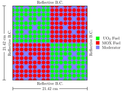
Test A is defined by the checker-board configuration formed by quarters of fuel assemblies. It is shown in Figure 2.2. There are assemblies with two kinds of fuels: (i) UO2 and (ii) mixed-oxide (MOX). The isotope compositions of model fuels and number densities of nuclides are presented in Tables 2.1 and 2.2. Each type of fuel pins has the same material properties. The fuel lattice pitch is 1.26 cm and the fuel pins have a radius of 1.08 cm. The space between fuel pins is filled with water. All boundaries are reflective. This problem is equivalent to the infinite spatial domain of two full assemblies next to each other.
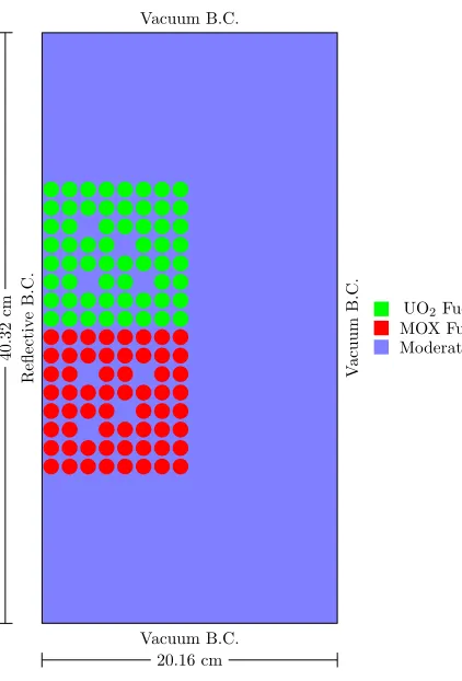
Test B (Figure 2.3) consists of the full-size MOX and UO2 assemblies from Test A with large area of water that models a reflector region. The configuration of this test is shown in Figure 3.3. It is similar to C5G7 benchmark [49]. The left and bottom boundaries are reflective. The top and right boundaries are vacuum.
Both tests are defined using 44-group cross sections from SCALE 6.1 data library [66]. Figure 2.5 demonstrates Σt,g,νf,gΣf,g, andχg for three different materials used in the tests. The group
data values are plotted versus midpoints of group energy intervals. The scattering matrices Σs,g→g0 are shown in Figure 2.6. The matrix elements are plotted versus the group indices.
Table 2.1: Isotope composition of UO2 fuel and number densities [1024 cm−3].
Nuclide 234U 235U 236U 238U 16O
Density 5.93×10⁻⁶ 7.04
×10−4 3.22
×10−6 2.44
×10−2 4.62
×10−2
Table 2.2: Isotope composition of MOX fuel and number densities [1024 cm−3].
Nuclide 234U 235U 238U 238Pu 239Pu
Density 2.60×10⁻⁷ 5.43
×10−5 2.14
×10−2 4.66
×10−5 1.02
×10−3
Nuclide 240Pu 241Pu 242Pu 16O
Density 4.83×10⁻⁴ 1.75
×10−4 1.32
×10−4 4.66
×10−2
eigenvalue and associated eigenfunction on the given fine energy grid are
||φ(s)−φ(s−1)||∞≤εφ||φ(s)||∞, (2.57)
k
(s)−k(s−1) ≤εkk
(s), (2.58)
where
||f||∞= max
i,j,g |fg,i,j|, (2.59)
iandj span the spatial mesh,g= 1, . . . , G,sis the index of the multigrid iteration cycle. The parameters of convergence criteria are εk=10−6 and εφ=10−6. The calculated multiplication
factors are (i)kef f = 1.0761 in Test A and (ii)kef f = 1.0455 in Test B.
Reflectiv e B.C. Reflectiv e B.C. Reflective B.C. Reflective B.C. 21.42 cm 21.42 cm MOX Fuel
UO2Fuel
Moderator
Figure 2: Test 1 geometry and configuration.
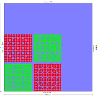
Reflectiv e B.C. V acuum B.C. Reflective B.C. Vacuum B.C. 64.26 cm 64.26 cm MOX Fuel UO2Fuel Moderator
Figure 3: Test 2 geometry and configuration.
MLD-3 [44,22,1]. The second grid has twenty groups with eleven fast and eleven thermal. The second grid is defined as pairs of the original groups.
MLD-4 [44,8,2,1].The four gird method uses both the eight-group and two-group grids defined above. MLD-5 [44,8,4,2,1]. The five gird method uses both the eight-, four-, and two-group grids defined
above.
With these multigrid methods we are trying to reduce the work in the low-order equations. The ”best” cycle is one that gives the minimum number of total groupwise solves.
The results from these two test problems with various cycles on the specified energy grids are sumarized in Tables 2 and??. The first column specifies the cycle algorithm and the second column lists the number of cycles until convergence. Columns 3-8 list the number of times the groupwise NDA equations were solved on each energy grid. The total number of groupwise solves is the sum of the NDA solves on all energy grids and the number of LO solves per group is the total divided by the 44 energy groups.
These two tables show that adding energy grids can reduce both the number of cycles and the total number of LO solves. This shows that the work is being shifted from the high dimensional grids to the lower dimensional grids. Going from two grids to any of the three grid sequences results is a significant reduction in the number of LO solves. Of the three grid methods for Test 1 the [44,8,1] sequence takes the least work with the MLD-3(2,1) cycle being the most efficient and for Test 2 the [44,4,1] with the MLD-3(1,1) cycle has the fewest LO solves. This set of three grid results show that few groups do not add much work, but they do not give as much improvement in the cycle. More groups can reduce the total number of cycles, but too many groups will increase the total number of LO solves. The four grid method with the (\)-cycle takes less work than any of the three grid methods. Performing nested cycles for this grid sequence only increases the cost of each cycle without reducing the total number of cycles. The five grid method has the same number of cycles as the four grid method, but the additional grid makes each cycle more expensive so it does takes a little more LO
Figures??show the convergence of the solution for select methods for both tests. These errors were calculated by comparing a running original grid solution to a reference solution. The running solution is
Figure 2.2: Geometry and configuration of test problem A.
Coarsening of energy grids is evaluated by the coupling of the equations between energy groups. This is done by analyzing the cross section data. There are two factors in the coupling, scattering and fission production. The group low-order equations (1.19) are coupled though the right-hand side that has the following form:
Rφ1 =B1φ1+ 1
kC1φ
1, (2.60)
whereB1 and C1 are defined by Eq. (2.11). The operatorR accounts for scattering and fission neutron-nuclide reactions. At a spatial position, the operator Ris defined by the matrix
Rg,g0 = Σs,g0→g+1
kχgνf,g0Σf,g0. (2.61)
![Figure 2.5:The 44-group neutron cross section data generated with SCALE 6.1 data library[66].](https://thumb-us.123doks.com/thumbv2/123dok_us/1595390.1196859/39.612.103.529.305.505/figure-group-neutron-cross-section-generated-scale-library.webp)