Multilevel Methods for Sparsification and Linear Arrangement Problems on Networks

Clemson University

TigerPrints

All Theses

Theses

5-2016

Multilevel Methods for Sparsification and Linear

Arrangement Problems on Networks

Emmanuel John

Clemson University, [email protected]

Follow this and additional works at:

https://tigerprints.clemson.edu/all_theses

This Thesis is brought to you for free and open access by the Theses at TigerPrints. It has been accepted for inclusion in All Theses by an authorized administrator of TigerPrints. For more information, please [email protected].

Recommended Citation

John, Emmanuel, "Multilevel Methods for Sparsification and Linear Arrangement Problems on Networks" (2016).All Theses. 2398. https://tigerprints.clemson.edu/all_theses/2398

M

ULTILEVEL

M

ETHODS FOR

S

PARSIFICATION AND

L

INEAR

A

RRANGEMENT

P

ROBLEMS ON

N

ETWORKS

A Thesis Presented to the Graduate School of

Clemson University In Partial Fulfillment of the Requirements for the Degree

Master of Science Computer Science by Emmanuel John May 2016 Accepted by:

Dr. Ilya Safro, Committee Chair Dr. Amy Apon

Dr. Brian Dean Dr. Hongxin Hu

Abstract

The computation of network properties such as diameter, centrality indices, and paths on networks may become a major bottleneck in the analysis of network if the network is large. Scalable approximation algorithms, heuristics and structure preserving network sparsification methods play an important role in mod-ern network analysis. In the first part of this thesis, we develop a robust network sparsification method that enables filtering of either, so called, long- and short-range edges or both. Edges are first ranked by their alge-braic distances and then sampled. Furthermore, we also combine this method with a multilevel framework to provide a multilevel sparsification framework that can control the sparsification process at different coarse-grained resolutions. Experimental results demonstrate an effectiveness of the proposed methods without significant loss in a quality of computed network properties.

In the second part of the thesis, we introduce asymmetric coarsening schemes for multilevel al-gorithms developed for linear arrangement problems. Effectiveness of the set of coarse variables, and the corresponding interpolation matrix is the central problem in any multigrid algorithm. We are pushing the boundaries of fast maximum weighted matching algorithms for coarsening schemes on graphs by introduc-ing novel ideas for asymmetric couplintroduc-ing between coarse and fine variables of the problem.

Dedication

To all African kids still striving to get a good education regardless of the challenges. To my father for leaving me a legacy through education.

Acknowledgments

My special thanks goes to my adviser Dr. Ilya Safro for helping to make this work possible and for helping me believe that I can do it. I want to say thank you to my parents for their unending love and support. I am also grateful to all my friends and family for all the care and support. My friends Kevin Jett, Mahi, and Mihidum encouraged me to go to grad school and even provided some financial support. A quick thank you to my lab colleagues Hayato and Ehsan - thank you for answering all my questions and for all your help. Many people along the way have contributed positively to my life. I cannot mention all the names but I will be forever grateful. Finally, I would like to thank all my committee members for their support and help in my research.

Table of Contents

List of Figures . . . vii

1 Introduction . . . 1

1.1 Background on Multiscale methods . . . 2

2 Single- and Multi-level Network Sparsification by Algebraic Distance . . . 5

2.1 Introduction . . . 5 2.2 Preliminaries . . . 9 2.3 Algebraic distance . . . 9 2.4 Single-level sparsification . . . 10 2.5 Multilevel sparsification . . . 11 2.6 Computational Results . . . 14 2.7 Normalized Sparsification . . . 23 2.8 Conclusions . . . 32

3 A Multilevel Algorithm for the Minimum 2-Sum Problem . . . 34

3.1 Introduction . . . 34

3.2 The Algorithm . . . 37

3.3 Results . . . 43

3.4 Conclusion . . . 45

List of Tables

2.1 Benchmark graphs . . . 16

2.2 Multiscale results for social networks 1 (SN1) graphs . . . 30

2.3 Multiscale results for social networks 2(SN2) graphs . . . 31

2.4 Multiscale results for biological (BIO) networks . . . 32

2.5 Multiscale results for citation (CIT) networks . . . 32

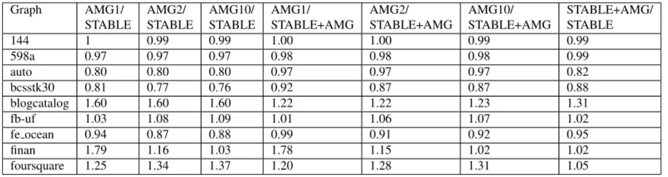
3.1 Results for multilevel minimum 2-sum solver for AMG, STABLE and STABLE+AMG . . . 44

List of Figures

1.1 Coarsening and Uncoarsening cycle of a multilevel algorithm . . . 3

2.1 An example of a small network with 3 dense clusters and sparse cuts between them (a). Sparsification of -weak connections will result in network presented in (b). Sparsification of -strong connections is presented in (c). . . 11

2.2 full-vcyle . . . 15 2.3 Social Networks 1 . . . 19 2.4 Social Networks 2 . . . 20 2.5 Citation Networks . . . 21 2.6 Biological Networks . . . 22 2.7 Social Networks 1 . . . 24 2.8 Social Networks 2 . . . 25 2.9 Citation Networks . . . 26 2.10 Biological Networks . . . 27

2.11 Comparison of LD and single-level algebraic distance methods. . . 29

2.13 runtime-parallel. . . 31

Chapter 1

Introduction

Many real world objects and the relationship between them can be modeled as networks which are represented as graphs in the computer systems and algorithms, where vertices represent the objects and edges abstract away the connection between them. For the purpose of this thesis, this definition of “real world” net-works would suffice. Problems in scheduling, transportation, VLSI and robotics benefit from being modeled as graph problems. Therefore, the capability afforded by graphs lead to algorithmic problems like searching, spanning trees, shortest path, flow problems and matching problems. Efficient implementations for some of these algorithms exists. However, many graph problems are computationally expensive (e.g., they can be NP-complete). Examples of such problems include graph partitioning, linear arrangement, and coloring. In particular, many versions of, so called, constrained cut-based problems such as partitioning, and clustering are computationally intractable. Quadratic, cubic (and even many nearly-linear time) approximation algorithms that produce suboptimal solutions with some guarantees become infeasible as the size of the input becomes large, so heuristics that provide approximate solutions in strictly linear time with no hidden coefficients are critical. Some of these problems benefit from the application of multiscale methods.

In this thesis, we focus on developing scalable algorithms for real world networks. First we introduce a method of graph sparsification that combines the algebraic distance of edges with a multilevel framework to filter the graph at various resolutions. We provide empirical results that show the preservation of many important structural properties of the original network. Secondly, we develop the minimum 2-sum solver introduced in [66] and extend the coarsening scheme with a stable matching algorithm to improve the solution for real world networks.

Thesis Structure

We begin this thesis with an overview of various methods applied in the domain. In Chapter 1.1, we provide a quick survey and background of multiscale methods. In Chapters 1.2-1.4, we provide an overview of stable matching, graph layout problems and sparsification. Chapter 2 of this thesis is based on an accepted journal paper [41]. The main focus of that chapter is graph sparsification. In Chapter 3, we develop an multilevel algorithm for the minimum 2-sum problem first introduced in [66] and extend the coarsening scheme with a stable matching algorithm.

1.1 Background on Multiscale methods

Data derived from complex networked systems in a form of weighted graphs can exhibit a dis-crepancy between the macro- and the microscopic scales. This is due to the difference in the underlying physical, biological or social models that describe the system at different scales. In many cases, it has been observed that complex and even non-deterministic systems can exhibit a much more ordered behavior at their coarse-grained resolutions. Multiscale methods are a class of algorithms that are employed in large scale computational and optimization problems to efficiently produce good approximate solutions in which the information from different scales of coarseness is used. Depending on the application and the domain, these methods are also referred to as multilevel, multiresolutional, and multigrid techniques. In this thesis we use them interchangeably.

Multiscale methods are typically applied to large-scale problems in which we can expect to interpo-late a solution of one variable to another. In other words, we can find dependencies between variables. An example is in the solving of partial differential equations where the change in the error at each iteration is small. Solving the entire problem in one shot can be prohibitively expensive. However, solving such problems at varying scales using multilevel algorithms, in which a solution in one point can be used to approximate another point, help to improve the solution and eliminate the waste to computational resources [9]

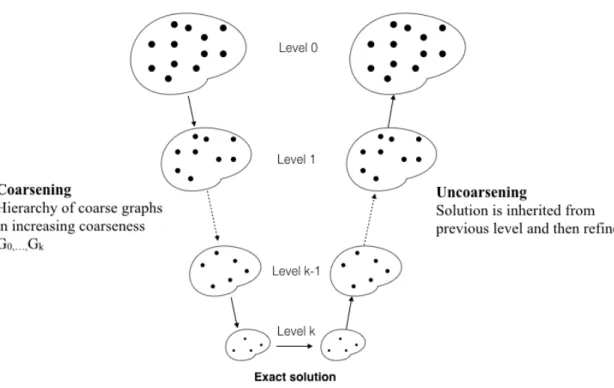
Our multilevel algorithms for graphs are inspired by the algebraic multigrid [14]. In graphs, the multilevel techniques work by aggregating parts or full vertices of the graph recursively to form a successive hierarchy of coarse graphs,G0,G1,...,Gk in increasing coarseness whereG0is the finest (original) graph

andGkis the coarsest graph. When the hierarchy of coarse representations is constructed, the computational problem is solved for the coarsest level and the solution is then refined and propagated to all the graphs staring from the coarsest to the finest. (See Figure 1.1). The idea is based on the intuition that vertices that have some

Figure 1.1: Coarsening and Uncoarsening cycle of a multilevel algorithm

“similarity, and closeness” properties might share similar solutions. For example, in the graph partitioning they may belong to the same part. This framework tends to accelerate global optimization algorithms and improve the quality of the solution.

The multiscale methods were first developed by Fedorenko and Bakhvalvov [4, 26, 27] and were employed in the solving of elliptic partial differential equations (PDE). The method was however extended by Brandt in his multi-level adaptive technique (MLAT) for solving boundary value problems [8]. Given their scalable nature, multiscale methods have since been applied to different computational or optimization problems in many fields. Applications of the method in previous studies have also been shown to significantly reduce the running times. In addition, it has been shown that local algorithms at each scale can be easily parallelized, making multiscale methods ideal candidates for parallel computers [11]. There is a long history of applying multilevel methods on graphs. Walshaw applied it to the drawing of large graphs [87]. Safro et al. applied the framework for solving the minimum linear arrangement problem in [65] to obtain approximate solutions in computationally efficient time frames. Examples include solvers for linear ordering problems [68] and network compression [70]. Numerous applications exist also for graph partitioning [34], modularity clustering [57], and graph visualization [84] Such problems as the traveling salesman, community detection

and graph layout benefit from a multilevel framework [9, 25, 68, 85]. The multilevel methods are also broadly applied in machine learning making different algorithms applicable on large-scale data. Examples include support vector machines [60], clustering [47], dimensionality reduction [72], and image segmentation [76]. An in-depth theoretical treatment of multilevel algorithms is beyond the scope of this thesis. For a deeper study, more literature on the topic can be found in [14, 15, 55]

Chapter 2

Single- and Multi-level Network

Sparsification by Algebraic Distance

2.1 Introduction

Networks are an abstract model of the relationships between discrete objects. Examples include networks of genes, consumers and generators in the power grid, and networks of friendships or followers in social communities. In order to study real world networks, they are often represented as graphs, where the vertices represent the objects and edges model the relationship or interaction between them. Modeling networks this way facilitates the analysis and understanding of many different structural properties of the underlying complex system. Several powerful software packages such as SNAP [50], Pajek[23], NetworkIt [80], NetworkX [31], and Gephi [6] have been developed to provide this capability. However, many complex networks are massive in size. For example, Facebook users post about 3.2 billion likes and comments each day [1], Twitter has more than 190 million users and about 65 million tweets are posted each day [88], and the human gene network contain several million edges [62]. Although, modeling and understanding these networks is very important in many application domains, the massive size of the network makes it often impractical to perform network analysis on the entire dataset.

In sparsification methods, we aim to select a representative sample of the corresponding graph such that some properties of the original graph are preserved. In other words, central to sparsification is the idea that if an algorithm depends on or computes the properties that are preserved in the sparsified graph,

we can expect that the results will be similar for the original graph [36] while the algorithm will perform much faster on the sparsified graph. Sampling is broadly being carried out in real world networks. Most network analytics consider just a sample in time of the networks under study which is usually the result of data collection limitations [1]. Thus, it is important to understand and develop scalable methods for sampling massive networks.

There are several motivating examples for network sparsification. One obvious example is in the domain of visualization. It is often computationally intensive to render huge graphs on a computer screen as well it is hard to visually analyze such graphs. Sparsification helps to visualize a sample of the graph that re-veals structural properties that would have been difficult to visualize and visually analyze in the original graph [46, 74]. The computational difficulty of visualization often arises from its objective, which requires solving a computational optimization problem [2, 38]. Another broad application is the reduction in the cost of com-putational network analysis. In computing the betweenness centrality of every node in a massive network, for example, by prioritizing what edges should be retained and what should be removed, it is possible to improve the running time of the algorithms at a very minimal cost in optimality [3]. Thirdly, graph sparsification can be applied to revealing hidden populations which are hard for researchers to find by just looking at the entire population. For example, Salganik et. al showed that when trying to sample the population of injection drug dealers, it is difficult to sample directly as this population is hidden and so specialized sampling algorithms are needed [73]. Methods applied usually involve starting out with a sample of the desired population and using that as a seed for revealing the other members of the sample population [36]. Existing methods include snowball sampling [29, 32] and respondent driven sampling [73]. In addition, in the case where there is an incomplete data, sampling can be used to estimate properties of the original graph. This is particularly useful in dynamic graphs [82], graph streaming algorithms [1] and collective classification [71].

There are several approaches to sampling a large graph while preserving the desired properties. An example involves formulating a mathematical programming problem to minimize the distance between the sparse graph and the original graph [36]. However, such approaches are often quite complex and running them might be costlier than running the algorithm on the larger graph. Spectral approximation algorithms also exist [79]. However, those algorithms are not very fast as well and often infeasible for large graphs [36] as they often involve hidden constants and require convergence in eigen-problems. The more common approaches are (1) vertex sampling, which involves selecting a number of vertices from the original graph and retaining the vertex-induced subgraph, and (2) edge sampling, which involves the selection of edges and corresponding edge-induced subgraph. Other variations of edge and vertex sampling have been developed

(see [36] for a full survey). In our method we focus on the edge sampling and also preserve the nodes from the original graph. In order to achieve this, we ensure that every node has at least one incident edge in the sparsified graph.

2.1.1 Strength of Connectivity in Sparsification

If the properties to be preserved are known beforehand, then, in many cases, it is possible to de-termine what kind of edges are important to preserve those properties and which ones are redundant. Thus, the sampling transformation can then be designed with the objective of retaining those edges. A general framework for sparsification involves: (1) ranking the edges and assigning each edge an edge score; and (2) sampling edges based on their scores [36]. Scoring edges provides a motivation for rating the strength of connection between two vertices. In particular, this is extremely important in weighted networks, where the weights can be approximate, noisy or even completely missing. Different types of the connection strength have been proposed for scoring edges. We refer the reader to [51] for a brief survey on the sparsification-relevant types of connectivity strength. The most sparsification-relevant to our work is a cohort of spectral methods widely used in theoretical computer science to sparsify dense graphs such that some spectral properties are preserved. These are usually cut-based properties that are formulated using Cheeger inequality. For example, Spielman et al. introduced the edge effective resistance [77]. The effective resistance is computed using the linear system solver [78] which runs inO(mlog15_{n)time which can be time consuming to be feasible. Another}

example is the vectorized PageRank [22]. Various interpretations of the diffusion have been proposed and analyzed [43, 83] for graph kernels. However, these methods usually suffer from impractical complexity.

Another relevant class of methods is based on the Jaccard index in which a similarity between two vertices is measured by computing the overlap in their neighborhoods. In [74], Satuluri et. al rated edges according to the local similarity sim(i, j) =|Ni\Nj|/|Ni[Nj|, whereNiis the neighborhood of nodei. This method was designed for clustering objectives assuming that nodes with larger shared neighborhoods are likely to belong to the same cluster. A global similarity threshold is then chosen for which edges are filtered. The authors also introduced a method for local sparsification in which they rate and filter edges per node by selecting the topde

i edges ranked by their similarity score, wheree2(0,1). Their method ensures that there is at least one edge per node after sparsification. We explore this property in our method. This sparsification technique can be computationally expensive since it requires counting the number of triangles an edge is a part of. The authors, however, provided an approximation for computing the similarity. Based on the work of Satuluri et al. [74], local degree method favors the retention of high degree nodes - also known

as hub nodes [51]. As in the local similarity, for each node, they include edges to the topde

i nodes. However, edges are sorted according to the degree of their neighbors in descending order. The main idea of this method is to keep edges in sparsified graph that leads to nodes with high degree. Additionally, vertex connectivity can be measured by the betweenness centrality, the shortest path length, the weight of substructures (such as spanning rooted forests, routes, overlapping paths that connect two vertices [18]) and algebraic distance [19] which we will discuss in Section 2.3.

2.1.2 Our Contribution

We introduce two methods for complex network sparsification that distinguish between strong and weak connectivity through neighborhoods of limited distance from the endpoints of edges. In some networks (such as those that include geospatial information), these types of connections can be interpreted as long- and short-range connections while in other (such as social networks) as inner- and outer-community connections. In both methods the sampling is based on the connectivity measured by the algebraic distance between nodes [19]. It generalizes the idea of methods that estimate the Jaccard coefficient for more distant neighborhoods through limited application of lazy random-walks (also known as algebraic distance [19]).

In the first method (the single level approach) we demonstrate multiple settings of filtering local and global connections with the sampling similar to [74]. In the second method we propose a multilevel algorithm that combines the single level approach with the multilevel framework [61] to sparsify graphs at different coarse-grained resolutions. We provide a robust method that can be tuned to preserve different net-work properties that are important in a variety of applications. The multi- and single level methods can both be used to either preserve the global structure or the local structure. The resulting sparsified networks are compared with the original network using following properties: degree distribution, clustering coefficient, number of connected components1_{, diameter, betweenness centrality, PageRank centrality, and modularity}

[56]. Evaluation of both methods is demonstrated through comparison of the aforementioned network prop-erties with those measured on the original network. Finally, we discuss how our method can be parallelized and show the running time in OpenMP implementation. The proposed methods are implemented and avail-able at [40].

1_{In many existing sparsification methods, the number of connected components is preserved “artificially”, i.e., even if the edge is}

marked for deletion, it is not deleted if it increases the number of connected components. Here we do not restrict our algorithms with such requirement.

2.2 Preliminaries

We denote the graph underlying a given network byG= (V, E, w), whereV is a set of vertices,E

is a set of edges, andw:E_!R 0is a weighting function onEthat represents the strength of connectivity

between two vertices. The graph is undirected, containing no self-loops and multi-edges. For each node

i 2 V we define its degree bydi and its neighbors byNi. The clustering coefficient is a measure of the probability that neighbors of a node are connected to each other [56]. Consequently, it is a measure of the degree to which nodes in a network tend to cluster [88]. The clustering coefficient of a nodeiis defined as ci = i/⌧i, where iis the number of triangle subgraphsiparticipates in, and⌧i =di(di 1)/2, i.e., the number of triples. The clustering coefficient of a graphGis defined as

CG= 1 |V0_| X i2V0 ci, (2.1) whereV0 _{={i2 V | d}

i >1}. The diameter of a graph is defined as the maximum distance shortest path among all pairs of vertices inGfrom the same connected component. The resulting sparsified networks are

compared with the original network using following properties: degree distribution, clustering coefficient, number of connected components2_{, diameter, betweenness centrality, PageRank centrality, and modularity}

[56]. We will use the Spearman Rank Correlation Coefficient (⇢) that is a measure of the correlation between

two distributions. It is defined as⇢= 1 (6Pp2

i)/(n(n2 1)), wherepi=xi yi, andxiandyiare the ranks computed from the scoresXiandYi.

2.3 Algebraic distance

In order to determine the strength of connection of edges for the purpose of sparsification, we use the algebraic distance introduced in [19, 61]. The algebraic distance of an edgeij (denoted by ij) is inter-preted as locally converged iterative process that propagates the weighted average of values fromNiandNj initialized by random numbers [19]. This expresses the strength of connectivity between two nodes through their local neighborhoods. The process is essentially a Jacobi overrelaxation (JOR) or a lazy random walk with limited number of steps (see Algorithm 1). The algebraic distance was successfully used in several al-gebraic multigrid algorithms [16, 52] and in multilevel algorithms for discrete optimization on graphs (such

2_{In many existing sparsification methods, the number of connected components is preserved “artificially”, i.e., even if the edge is}

marked for deletion, it is not deleted if it increases the number of connected components. Here we do not restrict our algorithms with such requirement.

as the minimum linear arrangement [61], and graph partitioning [69]) to reduce the order of interpolation that results in a sparsified coarse system.

Algorithm 1Algebraic distance implementation: ComputeAlgDist

1: Input:Parameter↵(in our experiments↵= 1/2)

2: ₈ij₂E Rij = 0

3: forr= 0,1,2, ...do .the number of test vectorsris small 4: ₈i2V x(0)i rand( 0.5,0.5)

5: fork= 0,1,2, ...do .the number of JOR iterationskis small 6: ₈i₂V x(_ik) ↵x(_ik 1)+ (1 ↵) P j2Niwijx (k 1) j P j2Niwij 7: end for 8: Rescalexback to( 0.5,0.5) 9: ₈ij2E Rij=Rij+ (xi xj)2 10: end for 11: return₈ij ₂E ij 1 p Rij+✏ . ✏is sufficiently small 12: ₈ij2E ij p ij di⇤dj .optional normalization

Other stationary iterative relaxations can also be applied in a similar setting but since JOR is implic-itly parallelizable using matrix-vector multiplications, we prefer to use it instead of other relaxations (such as Gauss-Seidel) that converge faster. Optionally, the algebraic distance can also be normalized by the square-root of the product of the weighted degrees of the two nodes to reduce extremely high strength of connection between hub nodes.

The algebraic distance will serve as the main criterion for choosing edges for sparsification in the al-gorithms below. Because it helps to distinguish between so called short- and long-range connections [19], we will use it to demonstrate different types of sparsification in which local and global properties are preserved correspondingly to the types of algebraic distances that we choose. The short-range connections (large values of ij) will be called -strong. The long-range connections (small values of ij) will be called -weak.

2.4 Single-level sparsification

In the single-level approach we demonstrate three types of sparsification in which we filter -weak, -strong edges and their mixture. In all of these cases, first, for each edge in the graph, we compute the algebraic distance. Then, for each nodei, we sample the topde

i neighbors ranked by their algebraic distances, wheree ₂ [0,1]. In this approach it is possible to sample for local or global structure preservation or a

combination of both. To preserve the global structure, we selectde

(a) Original network (b) Sparsified network by elimi-nating -weak connections (c) Sparsified network by elimi-nating -strong connections

Figure 2.1: An example of a small network with 3 dense clusters and sparse cuts between them (a). Sparsifi-cation of -weak connections will result in network presented in (b). SparsifiSparsifi-cation of -strong connections is presented in (c).

sparse graph (see Figure 2.1c). Similarly,de

istrongest connections are preserved to emphasize the importance of a local structure in the sparse graphs (see Figure 2.1b).

Algorithm 2Single-level sparsification: Sparsify(G)

1: Input:Sparsification parametere, GraphG 2: Output: Sparsified graphGsparse

3: Gsparse empty graph

4: COMPUTEALGEBRAICDISTANCES(G) 5: fori₂V do

6: SortNiby ijin ascending (or descending) order

7: Add topde

i edges toGsparse

8: end for 9: returnGsparse

It is also possible to partially preserve both global and local structures with a slight change in the algorithm, namely, by distributing the algebraic distances into bins, and sampling the edges from all bins. In order, to distribute the algebraic distances into bins, we define the bin widthh= 3p.35⇤

di , and the number of

binsk= (max ij min ij)/h, where is the standard deviation of algebraic distances.

2.5 Multilevel sparsification

The multilevel approach [14, 86] can be applied as a general framework for many different numerical methods. Most real-world instances are not completely random, i.e., a particular similarity or dependence

Algorithm 3Single-level sparsification with binning: SparsifyB(G)

1: Input:Sparsification parametere, GraphG 2: Output: Sparsified graphGsparse

3: Gsparse empty graph

4: COMPUTEALGEBRAICDISTANCES(G) 5: fori₂V do

6: DistributeNiinto bins, each bin corresponds to edges ...

7: Randomly select bins and edges up tode

i toGsparse

8: end for 9: returnGsparse

between variables exists and, thus, can partially be detected to reduce their number in complex computations. Here we introduce and advocate the use of multilevel approach as a general purpose framework for network sparsification. In the heart of the proposed method lies an idea to sparsify the network at multiple scales of coarseness which, in contrast to most existing sparsification methods that sample single edges, will allow to sample clusters of edges of different sizes and -weakness.

It is known that the topology of many complex networks is hierarchical (or multiscale) and, thus, of-ten might be self-dissimilar across scales [7, 39, 54, 89]. In such hierarchical representations, groups of nodes are aggregated into communities, which automatically bundles edges into coarse connections. Bundling the edges at different scales of coarseness will introduce different levels of -weakness for such coarse connec-tions which may or may not be required to be sparsified for the required analysis. For example, in the analysis of a social network, we may want to visualize only a certain type of edges that connect dense communities of small sizes, while connections between large communities and local inner connections are out of the scope. In the proposed framework, this can be achieved by creating a hierarchy of coarse representations, and spar-sifying at those levels that do not correspond to the desired communities. To create a multilevel framework we use the algebraic multigrid (AMG) aggregation strategy that was introduced in [65]. For simplicity, we do not split fine nodes across the aggregates (like in some optimization problems [65, 69]) but instead cover the graph with star-like structures and coarsen them. For the completeness of paper we briefly repeat the main components of the coarsening algorithm.

Given an original graphG, in the multilevel framework we recursively construct a hierarchy of

de-creasing size coarse graphsG0 =G, G1, ..., Gl. The original graph is gradually coarsened into the smaller graphs until the small enough graphGl is reached. The sparsification algorithm is then run on the coars-est level and the results (i.e., edges to eliminate for sparsification) are inherited by the finer graph and the uncoarsening continues untilG0is reached. In most cases, our discussion is focused on fine-to-coarse and

coarse-to-fine transformations of graphs and solutions, respectively. For this purpose, we denote the fine and coarse level graphs byGf = (Vf, Ef), andGc = (Vc, Ec), respectively. At each level, after sparsifying edges inherited fromGc, Algorithm 1 is applied to recompute algebraic distance onGf.

The Coarsening We begin with selecting a dominating set of seed nodesC⇢Vf that will serve as centers of future coarse nodes inVc. Setting initially F = Vf andC = ;, the selection is done by traversal of

F and moving toC such nodes that are not strongly coupled to those that are already inC. At each step

F_[C =Vf is preserved, and at the end the size ofVcis known, namely,|Vc| =|C|. AfterCis selected, nodes inF =V_\Care distributed to their aggregates according to the restriction operatorP _2{0,1_}|Vf|⇥|C|,

where PiJ = 8 > > > > > > > < > > > > > > > : 1 ifi2F, J=Ic ✓ argmaxj2C ij P k2C ik ◆ 1 ifi2C, J=Ic(i) 0 otherwise, (2.2) andIc(j)returns an index of coarse nodeJthat corresponds toj2C. Then, the Galerkin coarsen-ing creates a coarse graph LaplacianLc=PTLfP, whereLf is the Laplacian ofGf.

Coarsest Level At the coarsest level, we sparsify the edges by using the single-level Algorithm (3). These edges correspond to bundles of edge chains at the fine levels that connect the most distant regions in a graph, so if the goal is to preserve the global structure, the user should avoid of sparsification at deep coarse levels.

Uncoarsening We initialize the solution (sparsification) ofGf by uncoarsening the edges sparsified inGc. When the order of interpolation in the multilevel algorithm equals 1 (i.e., there is only one non-zero entry per row inP, see Eq. 2.2), each coarse edgeIJ 2Eccan bundle at most two types of edges inEf, namely, at most one edge that connect two seedsI 1

c (I)andIc 1(J), and possibly multiple edgespq 2 Ef such that P_pI 1

c (I) = 1, andPqIc1(J) = 1. If IJ is sparsified at the coarse level, then edges of both types

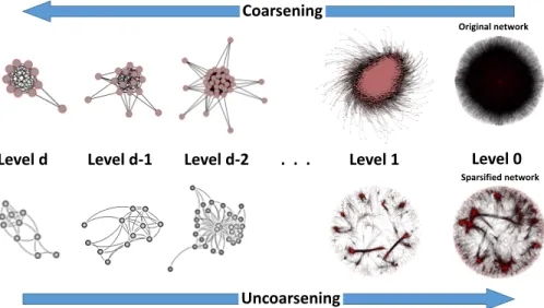
are sparsified at the fine level. After initialization of the fine level, we recompute algebraic distances to update the information about connectivity in the sparsified fine graph, and, then, more edges may or may not be sparsified at the fine level depending on the parameter settings. Full multilevel cycle is presented in Algorithm 4. Example of full multilevel cycle on a Facebook network (see fb-uf in Table 2.1) is shown in Figure 2.2.

Algorithm 4Multilevel sparsification of graph: MLSparsify

1: Input:fine graphGf = (Vf, Ef), vector of sparsification ratios

2: Output: sparse graphGs

f = (Vf, Efs)

3: functionML(Gf)

4: COMPUTEALGDIST(Gf)

5: if_|Vf|is small enoughthen

6: Es

f SPARSIFYB(Gf) .Sparsify coarse edges

7: else

8: CREATESEEDS(Gf) .Coarsening: seeds

9: ComputeP .Coarsening: restriction operator 10: Gc (Lc =PTLfP) .Coarsening: coarse graph

11: Gs

c MLSPARSIFY(Gc) .Recursive call to sparsify the next coarser level

12: Gsf UNCOARSEN(Gsc) .Sparsification of edges inherited from coarse level

13: COMPUTEALGDIST(Gs

f) .Algebraic distances are recomputed

14: Gs

f SPARSIFYB(Gsf) .Sparsification of current level edges

15: end if 16: end function 17: returnGs

f

2.6 Computational Results

Implementation and Evaluation We provide C++ implementation for both the single- and multilevel al-gorithms in [40]. For the comparison of original and sparsified networks, we employed methods implemented in NetworKit [80]. We experimented with varying degrees of sparsification, taking values oferanging from

0.1 to 0.9 (see Section 2.4). All numerical properties for the comparison are the averages over 10 runs with different random seeds for each parameter setting. The following parameter were used in computation of algebraic distance:R= 10,k= 40, and↵= 0.5. Their robustness is discussed in [19]. In addition, for the

single-level algorithm (Algorithm 3), we provide two sets of results for each graph, namely, with and without the normalization (see last step in Algorithm 1) of algebraic distance. In each case we experimented with sparsification of weak edges, strong edges and mixture of both.

In the multilevel algorithm (Algorithm 4), we experimented with sparsifying at the coarsest, middle and the finest levels. In our experiments, we split the number of levels in the multilevel algorithm into 3 equal segments, and choose a parameter, level-span which determine how many levels in each segment gets sparsified. We then sparsify one segment at a time and observe the corresponding network properties. For example, for a graph with 6 levels, with a level-span of 2, to sparsify the coarsest levels only we use the fol-lowing parameter configuration:(0.3,0.3, 1, 1, 1, 1), where a setting of 1indicates no sparsification

occurs at this level. Similarly, the middle and finest levels can be sparsified using( 1, 1,0.3,0.3, 1, 1),

Coarsening

Uncoarsening

Level 0

Level 1

Level d Level d-1 Level d-2 . . .

Original network

Sparsified network

Figure 2.2: Complete Sparsification V-Cycle

can specify any combination of settings for different levels. The sparisification ratio (ratio of number edges in the sparse graph to the number of edges in the original graph), is kept between 20% to 40% for each stage in order to make the results comparable. For the purpose of our study, we maintain a level span of 3.

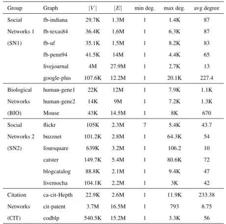
Datasets We experiment with 18 real-world networks (see Table 2.1), which for the purpose of our study we grouped into two groups of social networks, one group of citation networks (CIT) and one group of biological networks (BIO). We split the social networks into 2 groups (SN1, and SN2) - one consisting of Facebook net-works, Livejournal and Google+ (general purpose social networks), and the other consisting other consisting of Flickr, Buzznet, Foursquare, Catster, Blogcatalog and Livemocha. The graphs were retrieved from the NetworkRepository [63], the Koblenz [45], and the SNAP [49] collections. The size of the networks range between 1 million to 34 million edges.

Table 2.1: Benchmark graphs

Group Graph |V| |E| min deg. max deg. avg degree

Social fb-indiana 29.7K 1.3M 1 1.4K 87 Networks 1 fb-texas84 36.4K 1,6M 1 6.3K 87 (SN1) fb-uf 35.1K 1.5M 1 8.2K 83 fb-penn94 41.5K 14M 1 4.4K 65 livejournal 4M 27.9M 1 2.7K 13 google-plus 107.6K 12.2M 1 20.1K 227.4 Biological human-gene1 22K 12M 1 7.9K 1.1K Networks human-gene2 14K 9M 1 7.2K 1.3K (BIO) Mouse 43K 14.5M 1 8K 670 Social flickr 105K 2.3M 7 5.4K 43.7 Networks 2 buzznet 101.2K 2.8M 1 64.3K 54 (SN2) foursquare 639K 3.2M 1 106.2 10 catster 149.7K 5.4M 1 80.6K 72 blogcatalog 88.8K 2.1M 1 9.4K 47 livemocha 104.1K 2.2M 1 3K 42 Citation ca-cit-Hepth 22.9K 2.6M 1 11.9K 233.38 Networks cit-patent 3.7M 16.5M 1 793 8.75 (CIT) codblp 540.5K 15.2M 1 3.3K 56

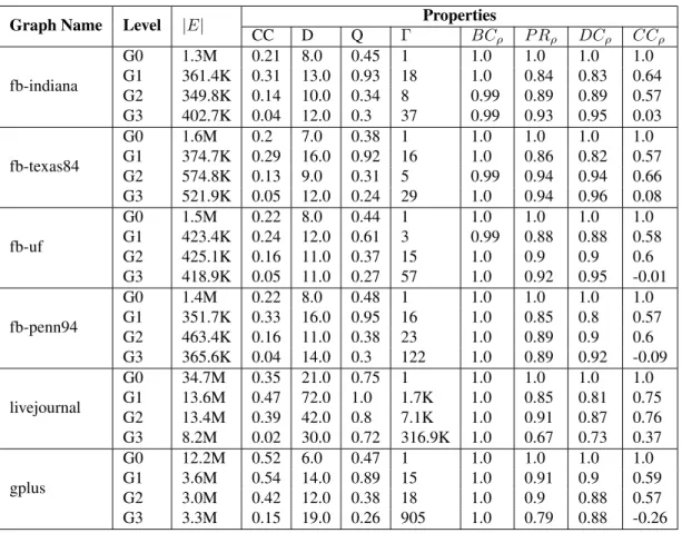
Methods of Comparison We studied various levels of sparsification while comparing the following prop-erties of the sparse graphGs, to those in the original graphGo. The single value properties are: (a)Diameter - We measure the ratio of the diameter inGoto the new diameter inGs(in plots “orig diameter/diameter”); (b)Number of connected components- we measure the ratio of the number of connected components inGs to that inGo(in plots “comp/orig comp”); (c)Modularity- we measure the ratio of modularity inGsto that ofGo(in plots “mod/orig mod”, Networkit [80] provides an implementation of the Louvain method). Certain network properties are represented better by their distributions over the nodes. In order to accurately compare the distributions, we use the Spearman rank correlation coefficient. This effectively, reveals how different the sparse graph is from the original in the context of these properties where a correlation value of 1 means they are perfectly correlated and correlation value of 0 means no correlation. The following distributions are compared using the Spearman rank: (a) Nodebetweeennesscentrality; (b)PageRankcentrality; (c)Degree distribution; and (d)Clustering coefficient distribution(ci). The method changes slightly in comparing node betweenness centrality. Considering that the cost of computing betweenness for large graphs is very

expensive, we make use of an approximate method provided by Networkit. However, to ensure accuracy we compute this 10 times and take average of the positional rankings and then compute the Spearman rank correlation.

2.6.1 Single-level Algorithm

The single-level algorithm was tested with both unnormalized and normalized algebraic distances. The results for unnormalized algebraic distance are presented in Figures 2.3, 2.4, 2.5, and 2.6 for groups SN1, SN2, CIT, and BIO, respectively. (The results for the normalized algebraic distance can be found in section 2.7.) In each figure, 3 columns, and 7 rows of plots are presented. In all 4 figures: (a) each column corresponds to the type of filtering, i.e., to the types of edges that retain after sparsification; (b) each row corresponds to the type of comparison. Each plot contains several colored curves that correspond to the respective graphs (see vertical legend). One point in each curve corresponds to an average of the measured comparison method over 10 runs for the corresponding edge ratio in each. The x- and y-axes correspond to the sparsification ratio and method of comparison, respectively. In the y-axis of betweenness, PageRank, degree, and clustering coefficient distribution centralities, the Spearman rank is denoted by⇢. For example, we examine the behavior of the degrees in social network Google+ in SN1 when -strong edges retain after sparsification. In Figure 2.3, we find a row “Degree centrality” (row 3). The results for retaining -strong edges are found in the third column. The black curve corresponds to Google+, where each point is an average of 10 runs.

Note: Most curves do not reach a visible zero of the x-axis. This is because the sparsification is interrupted when the number of edges becomes less than the number of nodes.

-weak edges Plots labelled as -weak (column 1) are results obtained by retaining only weak edges, when -weak edges are preferred during sparsification (i.e, -strong edges are deleted). In this type of sparsifica-tion, we expect that sparsification of the local structure will mostly dominate the sparsification of the global structure. Indeed, we observe that properties (such as the betweenness centrality, diameter, and the num-ber of components) that heavily depend on usually limited numnum-ber of long-range weak connections are well preserved.

-strong Plots labelled as -strong (column 3) are results obtained by retaining -strong edges and remov-ing -weak edges. By preferrremov-ing -strong edges durremov-ing sparsification, we attempt to preserve properties that

depends on the local structure of the graph. Such properties as clustering coefficient, pagerank and degree centrality survive sparsification better when this method is used. In particular, we can observe that the clus-tering coefficient (which is in many cases the reason for a strong community structure) is preserved at the level of⇡ 75%in SN1 when 70% of edges are removed (instead of⇡ 40%for -weak sparsification). A similar phenomena is observed in BIO. It is interesting to note that in SN2, in comparison to the -weak sparsification, the changes in the clustering coefficient are not significant.

Mixture sparsification In plots labelled as mixed, we maintain a balance between the -weak and -strong types of sparsification by preferring ensuring that both are sparsified. For such properties as the betweenness centrality, PageRank and degree centrality, the results are better for up to 20% sparsification ratio when com-pared to selecting either weak or strong edges. For such properties as the clustering coefficient, modularity, diameter and connected components, retaining both weak and strong edges provides results that is in between that produced by weak or strong edges sparsification.

fb-indiana fb-uf fb -te xa s8 4 fb-penn94 gplus lj

-weak Mixture -strong

Betweenness Centrality 0.2 0.4 0.6 0.8 1.0 Edge ratio 0.985 0.990 0.995 1.000 0.2 0.4 0.6 0.8 1.0 Edge ratio 0.992 0.994 0.996 0.998 1.000 0.2 0.4 0.6 0.8 1.0 Edge ratio 0.980 0.985 0.990 0.995 1.000 1.005 Clustering Coef ficient Distrib ution 0.2 0.4 0.6 0.8 1.0 Edge ratio 0.0 0.2 0.4 0.6 0.8 1.0 0.2 0.4 0.6 0.8 1.0 Edge ratio 0.0 0.2 0.4 0.6 0.8 1.0 0.2 0.4 0.6 0.8 1.0 Edge ratio 0.0 0.2 0.4 0.6 0.8 1.0 De gree Centrality 0.2 0.4 0.6 0.8 1.0 Edge ratio 0.4 0.6 0.8 1.0 1.2 0.2 0.4 0.6 0.8 1.0 Edge ratio 0.92 0.94 0.96 0.98 1.00 0.2 0.4 0.6 0.8 1.0 Edge ratio 0.5 0.6 0.7 0.8 0.9 1.0 Diameter 0.2 0.4 0.6 0.8 1.0 Edge ratio 0.55 0.60 0.65 0.70 0.75 0.80 0.85 0.90 0.95 1.00 Orig diameter/diameter 0.2 0.4 0.6 0.8 1.0 Edge ratio 0.55 0.60 0.65 0.70 0.75 0.80 0.85 0.90 0.95 1.00 Orig diameter/diameter 0.2 0.4 0.6 0.8 1.0 Edge ratio 0.0 0.2 0.4 0.6 0.8 1.0 Orig diameter/diameter Components 0.2 0.4 0.6 0.8 1.0 Edge ratio 0 20 40 60 80 100 120 comp /orig comp 0.2 0.4 0.6 0.8 1.0 Edge ratio 0 200 400 600 800 1000 1200 1400 comp /orig comp 0.2 0.4 0.6 0.8 1.0 Edge ratio 0 5000 10000 15000 20000 25000 30000 35000 comp /orig comp Modularity 0.2 0.4 0.6 0.8 1.0 Edge ratio 0.7 0.8 0.9 1.0 1.1 1.2 1.3 1.4 1.5 1.6 mod/orig mod 0.2 0.4 0.6 0.8 1.0 Edge ratio 0.9 1.0 1.1 1.2 1.3 1.4 1.5 1.6 mod/orig mod 0.2 0.4 0.6 0.8 1.0 Edge ratio 1.0 1.2 1.4 1.6 1.8 2.0 2.2 mod/orig mod Pagerank 0.2 0.4 0.6 0.8 1.0 Edge ratio 0.2 0.4 0.6 0.8 1.0 1.2 0.2 0.4 0.6 0.8 1.0 Edge ratio 0.90 0.92 0.94 0.96 0.98 1.00 0.2 0.4 0.6 0.8 1.0 Edge ratio 0.5 0.6 0.7 0.8 0.9 1.0

fli ckr fo ur sq ua re ca tst er bu zzn et bl og ca ta lo g liv em och a

-weak Mixture -strong

Betweenness Centrality 0.2 0.4 0.6 0.8 1.0 Edge ratio 0.996 0.998 1.000 0.2 0.3 0.4 0.5 0.6 0.7 0.8 0.9 1.0 Edge ratio 0.997 0.998 0.999 1.000 0.2 0.4 0.6 0.8 1.0 Edge ratio 0.996 0.998 1.000 Clustering Coef ficient Distrib ution 0.2 0.4 0.6 0.8 1.0 Edge ratio 0.2 0.4 0.6 0.8 1.0 1.2 0.2 0.3 0.4 0.5 0.6 0.7 0.8 0.9 1.0 Edge ratio 0.2 0.4 0.6 0.8 1.0 1.2 0.2 0.4 0.6 0.8 1.0 Edge ratio 0.2 0.4 0.6 0.8 1.0 1.2 De gree Centrality 0.2 0.4 0.6 0.8 1.0 Edge ratio 0.2 0.4 0.6 0.8 1.0 1.2 0.2 0.3 0.4 0.5 0.6 0.7 0.8 0.9 1.0 Edge ratio 0.80 0.85 0.90 0.95 1.00 0.2 0.4 0.6 0.8 1.0 Edge ratio 0.5 0.6 0.7 0.8 0.9 1.0 Diameter 0.2 0.4 0.6 0.8 1.0 Edge ratio 0.3 0.4 0.5 0.6 0.7 0.8 0.9 1.0 Orig diameter/diameter 0.2 0.3 0.4 0.5 0.6 0.7 0.8 0.9 1.0 Edge ratio 0.3 0.4 0.5 0.6 0.7 0.8 0.9 1.0 Orig diameter/diameter 0.2 0.4 0.6 0.8 1.0 Edge ratio 0.1 0.2 0.3 0.4 0.5 0.6 0.7 0.8 0.9 1.0 Orig diameter/diameter Components 0.2 0.4 0.6 0.8 1.0 Edge ratio 1.00 1.02 1.04 1.06 1.08 1.10 1.12 comp /orig comp 0.2 0.3 0.4 0.5 0.6 0.7 0.8 0.9 1.0 Edge ratio 1.00 1.05 1.10 1.15 1.20 comp /orig comp 0.2 0.4 0.6 0.8 1.0 Edge ratio 0 200 400 600 800 1000 1200 comp /orig comp Modularity 0.2 0.4 0.6 0.8 1.0 Edge ratio 0.6 0.8 1.0 1.2 1.4 1.6 1.8 2.0 2.2 mod/orig mod 0.2 0.3 0.4 0.5 0.6 0.7 0.8 0.9 1.0 Edge ratio 1.0 1.2 1.4 1.6 1.8 mod/orig mod 0.2 0.4 0.6 0.8 1.0 Edge ratio 1.0 1.2 1.4 1.6 1.8 2.0 2.2 2.4 2.6 mod/orig mod Pagerank 0.2 0.4 0.6 0.8 1.0 Edge ratio 0.2 0.4 0.6 0.8 1.0 1.2 0.2 0.3 0.4 0.5 0.6 0.7 0.8 0.9 1.0 Edge ratio 0.80 0.85 0.90 0.95 1.00 0.2 0.4 0.6 0.8 1.0 Edge ratio 0.2 0.4 0.6 0.8 1.0 1.2 20

ca -ci t-H ep th co db lp ci t-p at en t

-weak Mixture -strong

Betweenness Centrality 0.2 0.4 0.6 0.8 1.0 Edge ratio 0.985 0.990 0.995 1.000 0.2 0.4 0.6 0.8 1.0 Edge ratio 0.990 0.995 1.000 0.2 0.4 0.6 0.8 1.0 Edge ratio 0.96 0.97 0.98 0.99 1.00 Clustering Coef ficient Distrib ution 0.2 0.4 0.6 0.8 1.0 Edge ratio 0.0 0.2 0.4 0.6 0.8 1.0 0.2 0.4 0.6 0.8 1.0 Edge ratio 0.2 0.4 0.6 0.8 1.0 1.2 0.2 0.4 0.6 0.8 1.0 Edge ratio 0.0 0.2 0.4 0.6 0.8 1.0 De gree Centrality 0.2 0.4 0.6 0.8 1.0 Edge ratio 0.0 0.2 0.4 0.6 0.8 1.0 0.2 0.4 0.6 0.8 1.0 Edge ratio 0.6 0.7 0.8 0.9 1.0 0.2 0.4 0.6 0.8 1.0 Edge ratio 0.2 0.4 0.6 0.8 1.0 1.2 Diameter 0.2 0.4 0.6 0.8 1.0 Edge ratio 0.60 0.65 0.70 0.75 0.80 0.85 0.90 0.95 1.00 Orig diameter/diameter 0.2 0.4 0.6 0.8 1.0 Edge ratio 0.75 0.80 0.85 0.90 0.95 1.00 1.05 Orig diameter/diameter 0.2 0.4 0.6 0.8 1.0 Edge ratio 0.1 0.2 0.3 0.4 0.5 0.6 0.7 0.8 0.9 1.0 Orig diameter/diameter Components 0.2 0.4 0.6 0.8 1.0 Edge ratio 0 50 100 150 200 250 300 350 comp /orig comp 0.2 0.4 0.6 0.8 1.0 Edge ratio 0 10 20 30 40 50 60 70 80 90 comp /orig comp 0.2 0.4 0.6 0.8 1.0 Edge ratio 0 2000 4000 6000 8000 10000 12000 14000 comp /orig comp Modularity 0.2 0.4 0.6 0.8 1.0 Edge ratio 0.8 1.0 1.2 1.4 1.6 1.8 mod/orig mod 0.2 0.4 0.6 0.8 1.0 Edge ratio 0.9 1.0 1.1 1.2 1.3 1.4 1.5 1.6 1.7 mod/orig mod 0.2 0.4 0.6 0.8 1.0 Edge ratio 1.0 1.2 1.4 1.6 1.8 2.0 2.2 2.4 mod/orig mod Pagerank 0.2 0.4 0.6 0.8 1.0 Edge ratio 0.5 0.0 0.5 1.0 0.2 0.4 0.6 0.8 1.0 Edge ratio 0.6 0.7 0.8 0.9 1.0 0.2 0.4 0.6 0.8 1.0 Edge ratio 0.0 0.2 0.4 0.6 0.8 1.0 21

human1

human2

m

ou

se

-weak Mixture -strong

Betweenness Centrality 0.0 0.2 0.4 0.6 0.8 1.0 Edge ratio 0.98 0.99 1.00 0.2 0.4 0.6 0.8 1.0 Edge ratio 0.990 0.995 1.000 0.0 0.2 0.4 0.6 0.8 1.0 Edge ratio 0.95 0.96 0.97 0.98 0.99 1.00 Clustering Coef ficient Distrib ution 0.0 0.2 0.4 0.6 0.8 1.0 Edge ratio 0.5 0.0 0.5 1.0 0.2 0.4 0.6 0.8 1.0 Edge ratio 0.0 0.2 0.4 0.6 0.8 1.0 0.0 0.2 0.4 0.6 0.8 1.0 Edge ratio 0.0 0.2 0.4 0.6 0.8 1.0 De gree Centrality 0.0 0.2 0.4 0.6 0.8 1.0 Edge ratio 0.4 0.6 0.8 1.0 1.2 0.2 0.4 0.6 0.8 1.0 Edge ratio 0.95 0.96 0.97 0.98 0.99 1.00 0.0 0.2 0.4 0.6 0.8 1.0 Edge ratio 0.7 0.8 0.9 1.0 Diameter 0.0 0.2 0.4 0.6 0.8 1.0 Edge ratio 0.60 0.65 0.70 0.75 0.80 0.85 0.90 0.95 1.00 Orig diameter/diameter 0.2 0.4 0.6 0.8 1.0 Edge ratio 0.75 0.80 0.85 0.90 0.95 1.00 1.05 Orig diameter/diameter 0.0 0.2 0.4 0.6 0.8 1.0 Edge ratio 0.1 0.2 0.3 0.4 0.5 0.6 0.7 0.8 0.9 1.0 Orig diameter/diameter Components 0.0 0.2 0.4 0.6 0.8 1.0 Edge ratio 1.00 1.01 1.02 1.03 1.04 1.05 comp /orig comp 0.2 0.4 0.6 0.8 1.0 Edge ratio 1.000 1.005 1.010 1.015 1.020 1.025 comp /orig comp 0.0 0.2 0.4 0.6 0.8 1.0 Edge ratio 1.00 1.05 1.10 1.15 1.20 1.25 comp /orig comp Modularity 0.0 0.2 0.4 0.6 0.8 1.0 Edge ratio 0.8 1.0 1.2 1.4 1.6 1.8 2.0 2.2 mod/orig mod 0.2 0.4 0.6 0.8 1.0 Edge ratio 1.0 1.2 1.4 1.6 1.8 2.0 2.2 2.4 mod/orig mod 0.0 0.2 0.4 0.6 0.8 1.0 Edge ratio 1.0 1.5 2.0 2.5 3.0 mod/orig mod Pagerank 0.0 0.2 0.4 0.6 0.8 1.0 Edge ratio 0.2 0.4 0.6 0.8 1.0 1.2 0.2 0.4 0.6 0.8 1.0 Edge ratio 0.92 0.94 0.96 0.98 1.00 0.0 0.2 0.4 0.6 0.8 1.0 Edge ratio 0.7 0.8 0.9 1.0 22

2.7 Normalized Sparsification

We experimented with the single-level algorithm that employ normalized algebraic distances (see line 15 of Algorithm 1). The purpose of this normalization is to decrease the strength of connection expressed in the algebraic distance between hubs. The normalization results show that normalizing the algebraic dis-tance further improves properties that are sensitive to the existence of weak edges. Example are diameter and connected components. As seen in the plots for diameter (see -weak column in Figures 2.7, 2.8, 2.9, and 2.10), the minimum edge ratio before the diameter deteriorates is further improved. Similarly for the number of components the number of components for the smallest sparse graph is reduced and some case kept constant as seen in -weak column in Figures 2.7, 2.8, 2.9, and 2.10). Such properties as local clustering coefficient, degree centrality, and PageRank that do not depend on global edges are relatively unaffected.

fb-indiana fb-uf fb -te xa s8 4 fb-penn94 gplus lj

-weak Mixture -strong

Betweenness Centrality 0.2 0.4 0.6 0.8 1.0 Edge ratio 0.985 0.990 0.995 1.000 0.2 0.4 0.6 0.8 1.0 Edge ratio 0.992 0.994 0.996 0.998 1.000 0.2 0.4 0.6 0.8 1.0 Edge ratio 0.985 0.990 0.995 1.000 Clustering Coef ficient Distrib ution 0.2 0.4 0.6 0.8 1.0 Edge ratio 0.0 0.2 0.4 0.6 0.8 1.0 0.2 0.4 0.6 0.8 1.0 Edge ratio 0.0 0.2 0.4 0.6 0.8 1.0 0.2 0.4 0.6 0.8 1.0 Edge ratio 0.0 0.2 0.4 0.6 0.8 1.0 De gree Centrality 0.2 0.4 0.6 0.8 1.0 Edge ratio 0.6 0.7 0.8 0.9 1.0 0.2 0.4 0.6 0.8 1.0 Edge ratio 0.80 0.85 0.90 0.95 1.00 0.2 0.4 0.6 0.8 1.0 Edge ratio 0.5 0.0 0.5 1.0 Diameter 0.2 0.4 0.6 0.8 1.0 Edge ratio 0.70 0.75 0.80 0.85 0.90 0.95 1.00 Orig diameter/diameter 0.2 0.4 0.6 0.8 1.0 Edge ratio 0.5 0.6 0.7 0.8 0.9 1.0 1.1 Orig diameter/diameter 0.2 0.4 0.6 0.8 1.0 Edge ratio 0.1 0.2 0.3 0.4 0.5 0.6 0.7 0.8 0.9 1.0 Orig diameter/diameter Components 0.2 0.4 0.6 0.8 1.0 Edge ratio 1.0 1.5 2.0 2.5 3.0 3.5 4.0 4.5 5.0 5.5 comp /orig comp 0.2 0.4 0.6 0.8 1.0 Edge ratio 0 500 1000 1500 2000 comp /orig comp 0.2 0.4 0.6 0.8 1.0 Edge ratio 0 5000 10000 15000 20000 25000 30000 35000 comp /orig comp Modularity 0.2 0.4 0.6 0.8 1.0 Edge ratio 0.6 0.7 0.8 0.9 1.0 1.1 1.2 1.3 1.4 1.5 mod/orig mod 0.2 0.4 0.6 0.8 1.0 Edge ratio 1.0 1.1 1.2 1.3 1.4 1.5 1.6 mod/orig mod 0.2 0.4 0.6 0.8 1.0 Edge ratio 1.0 1.2 1.4 1.6 1.8 2.0 mod/orig mod Pagerank 0.2 0.4 0.6 0.8 1.0 Edge ratio 0.0 0.2 0.4 0.6 0.8 1.0 0.2 0.4 0.6 0.8 1.0 Edge ratio 0.80 0.85 0.90 0.95 1.00 0.2 0.4 0.6 0.8 1.0 Edge ratio 0.5 0.0 0.5 1.0 24

fli ckr fo ur sq ua re ca tst er bu zzn et bl og ca ta lo g liv em och a

-weak Mixture -strong

Betweenness Centrality 0.2 0.4 0.6 0.8 1.0 Edge ratio 0.997 0.998 0.999 1.000 0.2 0.3 0.4 0.5 0.6 0.7 0.8 0.9 1.0 Edge ratio 0.997 0.998 0.999 1.000 0.2 0.4 0.6 0.8 1.0 Edge ratio 0.994 0.996 0.998 1.000 Clustering Coef ficient Distrib ution 0.2 0.4 0.6 0.8 1.0 Edge ratio 0.2 0.4 0.6 0.8 1.0 1.2 0.2 0.3 0.4 0.5 0.6 0.7 0.8 0.9 1.0 Edge ratio 0.2 0.4 0.6 0.8 1.0 1.2 0.2 0.4 0.6 0.8 1.0 Edge ratio 0.2 0.4 0.6 0.8 1.0 1.2 De gree Centrality 0.2 0.4 0.6 0.8 1.0 Edge ratio 0.4 0.6 0.8 1.0 1.2 0.2 0.3 0.4 0.5 0.6 0.7 0.8 0.9 1.0 Edge ratio 0.75 0.80 0.85 0.90 0.95 1.00 0.2 0.4 0.6 0.8 1.0 Edge ratio 0.2 0.4 0.6 0.8 1.0 1.2 Diameter 0.2 0.4 0.6 0.8 1.0 Edge ratio 0.55 0.60 0.65 0.70 0.75 0.80 0.85 0.90 0.95 1.00 Orig diameter/diameter 0.2 0.3 0.4 0.5 0.6 0.7 0.8 0.9 1.0 Edge ratio 0.3 0.4 0.5 0.6 0.7 0.8 0.9 1.0 Orig diameter/diameter 0.2 0.4 0.6 0.8 1.0 Edge ratio 0.1 0.2 0.3 0.4 0.5 0.6 0.7 0.8 0.9 1.0 Orig diameter/diameter Components 0.2 0.4 0.6 0.8 1.0 Edge ratio 0.94 0.96 0.98 1.00 1.02 1.04 1.06 comp /orig comp 0.2 0.3 0.4 0.5 0.6 0.7 0.8 0.9 1.0 Edge ratio 1.0 1.1 1.2 1.3 1.4 1.5 1.6 1.7 1.8 1.9 comp /orig comp 0.2 0.4 0.6 0.8 1.0 Edge ratio 0 200 400 600 800 1000 comp /orig comp Modularity 0.2 0.4 0.6 0.8 1.0 Edge ratio 0.6 0.8 1.0 1.2 1.4 1.6 1.8 2.0 2.2 mod/orig mod 0.2 0.3 0.4 0.5 0.6 0.7 0.8 0.9 1.0 Edge ratio 1.0 1.2 1.4 1.6 1.8 mod/orig mod 0.2 0.4 0.6 0.8 1.0 Edge ratio 1.0 1.2 1.4 1.6 1.8 2.0 2.2 2.4 mod/orig mod Pagerank 0.2 0.4 0.6 0.8 1.0 Edge ratio 0.5 0.0 0.5 1.0 0.2 0.3 0.4 0.5 0.6 0.7 0.8 0.9 1.0 Edge ratio 0.75 0.80 0.85 0.90 0.95 1.00 0.2 0.4 0.6 0.8 1.0 Edge ratio 0.4 0.6 0.8 1.0 1.2 25

ca -ci t-H ep th co db lp ci t-p at en t

-weak Mixture -strong

Betweenness Centrality 0.2 0.4 0.6 0.8 1.0 Edge ratio 0.992 0.994 0.996 0.998 1.000 0.2 0.4 0.6 0.8 1.0 Edge ratio 0.990 0.995 1.000 0.2 0.4 0.6 0.8 1.0 Edge ratio 0.98 0.99 1.00 Clustering Coef ficient Distrib ution 0.2 0.4 0.6 0.8 1.0 Edge ratio 0.5 0.0 0.5 1.0 0.2 0.4 0.6 0.8 1.0 Edge ratio 0.2 0.4 0.6 0.8 1.0 1.2 0.2 0.4 0.6 0.8 1.0 Edge ratio 0.0 0.2 0.4 0.6 0.8 1.0 De gree Centrality 0.2 0.4 0.6 0.8 1.0 Edge ratio 0.2 0.4 0.6 0.8 1.0 1.2 0.2 0.4 0.6 0.8 1.0 Edge ratio 0.6 0.7 0.8 0.9 1.0 0.2 0.4 0.6 0.8 1.0 Edge ratio 0.5 0.0 0.5 1.0 Diameter 0.2 0.4 0.6 0.8 1.0 Edge ratio 0.82 0.84 0.86 0.88 0.90 0.92 0.94 0.96 0.98 1.00 Orig diameter/diameter 0.2 0.4 0.6 0.8 1.0 Edge ratio 0.70 0.75 0.80 0.85 0.90 0.95 1.00 Orig diameter/diameter 0.2 0.4 0.6 0.8 1.0 Edge ratio 0.1 0.2 0.3 0.4 0.5 0.6 0.7 0.8 0.9 1.0 Orig diameter/diameter Components 0.2 0.4 0.6 0.8 1.0 Edge ratio 0 5 10 15 20 25 30 35 40 45 comp /orig comp 0.2 0.4 0.6 0.8 1.0 Edge ratio 0 20 40 60 80 100 120 comp /orig comp 0.2 0.4 0.6 0.8 1.0 Edge ratio 0 2000 4000 6000 8000 10000 12000 comp /orig comp Modularity 0.2 0.4 0.6 0.8 1.0 Edge ratio 0.8 1.0 1.2 1.4 1.6 mod/orig mod 0.2 0.4 0.6 0.8 1.0 Edge ratio 0.9 1.0 1.1 1.2 1.3 1.4 1.5 1.6 1.7 mod/orig mod 0.2 0.4 0.6 0.8 1.0 Edge ratio 1.0 1.2 1.4 1.6 1.8 2.0 2.2 mod/orig mod Pagerank 0.2 0.4 0.6 0.8 1.0 Edge ratio 0.5 0.0 0.5 1.0 0.2 0.4 0.6 0.8 1.0 Edge ratio 0.5 0.6 0.7 0.8 0.9 1.0 0.2 0.4 0.6 0.8 1.0 Edge ratio 0.5 0.0 0.5 1.0 26

human1

human2

m

ou

se

-weak Mixture -strong

Betweenness Centrality 0.0 0.2 0.4 0.6 0.8 1.0 Edge ratio 0.980 0.985 0.990 0.995 1.000 1.005 0.2 0.4 0.6 0.8 1.0 Edge ratio 0.990 0.995 1.000 0.0 0.2 0.4 0.6 0.8 1.0 Edge ratio 0.97 0.98 0.99 1.00 Clustering Coef ficient Distrib ution 0.0 0.2 0.4 0.6 0.8 1.0 Edge ratio 0.5 0.0 0.5 1.0 0.2 0.4 0.6 0.8 1.0 Edge ratio 0.0 0.2 0.4 0.6 0.8 1.0 0.0 0.2 0.4 0.6 0.8 1.0 Edge ratio 0.5 0.0 0.5 1.0 De gree Centrality 0.0 0.2 0.4 0.6 0.8 1.0 Edge ratio 0.6 0.7 0.8 0.9 1.0 0.2 0.4 0.6 0.8 1.0 Edge ratio 0.92 0.94 0.96 0.98 1.00 0.0 0.2 0.4 0.6 0.8 1.0 Edge ratio 0.2 0.4 0.6 0.8 1.0 1.2 Diameter 0.0 0.2 0.4 0.6 0.8 1.0 Edge ratio 0.70 0.75 0.80 0.85 0.90 0.95 1.00 Orig diameter/diameter 0.2 0.4 0.6 0.8 1.0 Edge ratio 0.75 0.80 0.85 0.90 0.95 1.00 1.05 Orig diameter/diameter 0.0 0.2 0.4 0.6 0.8 1.0 Edge ratio 0.2 0.3 0.4 0.5 0.6 0.7 0.8 0.9 1.0 Orig diameter/diameter Components 0.0 0.2 0.4 0.6 0.8 1.0 Edge ratio 0.94 0.96 0.98 1.00 1.02 1.04 1.06 comp /orig comp 0.2 0.4 0.6 0.8 1.0 Edge ratio 1.000 1.005 1.010 1.015 1.020 1.025 1.030 1.035 comp /orig comp 0.0 0.2 0.4 0.6 0.8 1.0 Edge ratio 1.00 1.05 1.10 1.15 1.20 1.25 1.30 comp /orig comp Modularity 0.0 0.2 0.4 0.6 0.8 1.0 Edge ratio 0.6 0.8 1.0 1.2 1.4 1.6 1.8 2.0 2.2 mod/orig mod 0.2 0.4 0.6 0.8 1.0 Edge ratio 1.0 1.2 1.4 1.6 1.8 2.0 2.2 2.4 mod/orig mod 0.0 0.2 0.4 0.6 0.8 1.0 Edge ratio 1.0 1.5 2.0 2.5 3.0 mod/orig mod Pagerank 0.0 0.2 0.4 0.6 0.8 1.0 Edge ratio 0.5 0.6 0.7 0.8 0.9 1.0 0.2 0.4 0.6 0.8 1.0 Edge ratio 0.90 0.92 0.94 0.96 0.98 1.00 0.0 0.2 0.4 0.6 0.8 1.0 Edge ratio 0.0 0.2 0.4 0.6 0.8 1.0 27

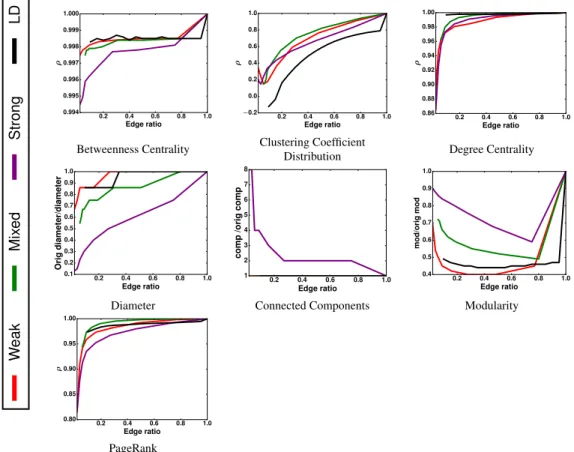
Comparing with Local Degree In the introduction, we mentioned the Local Degree method (LD) [51] which favors the retention of edges participating in hubs (nodes with high degree). In order to compare our method to LD, we ran the single level algorithm for retaining weak edges, strong edges and a mixture of both on the Google+ graph (google-plus in Table 2.1). Same set of network properties discussed earlier in this section were used for comparison. For betweenness centrality, degree centrality, local clustering coefficient and PageRank, we plot the Spearman rank correlation against the edge ratio. Figure 2.11 shows the plots of -weak, -strong, mixed and local degree(LD) for each property. The results are similar for betweenness centrality, degree centrality and PageRank. However, for such properties as modularity and clustering co-efficient, the algebraic d