ABSTRACT
JIANG, HANSI. Modularity Component Analysis. (Under the direction of Carl Meyer.)
In data clustering when high dimensional data is involved it is often necessary to cluster the data while reducing the number of dimensions. The principal component analysis (PCA) is a very popular analysis tool to achieve the goals, but one drawback of PCA is that the sparsity of the data may be destroyed while centering. Another data clustering method, the modularity clustering algorithm, does not require data centering, but the theory requires a bipartition of the data and a hierarchy has to be built if the number of clusters is more than two.
©Copyright 2016 by Hansi Jiang
Modularity Component Analysis
by Hansi Jiang
A dissertation submitted to the Graduate Faculty of North Carolina State University
in partial fulfillment of the requirements for the Degree of
Doctor of Philosophy
Applied Mathematics
Raleigh, North Carolina 2016
APPROVED BY:
Zhilin Li Shaina Race
Ernie Stitzinger Carl Meyer
DEDICATION
BIOGRAPHY
ACKNOWLEDGEMENTS
First, I would like to thank my advisor, Prof. Carl Meyer. He is a great mathematician and educator. I deeply appreciate his patience, encouragement, and the tremendous help in my research and my life. I also want to thank his wife, Mrs. Meyer, for caring about me and the delicious dinners.
Next, I want to thank the other three professors that in my committee. Prof. Li always cares about my life and my study. Prof. Stitzinger helped me a lot in many issues in the department. Prof. Race is always there to help.
I also appreciate Ralph Abbey and Phuong Hoang for reading this dissertation and the valuable feedbacks. Thank Le Li for the suggestions about preparing for graduation. Thank Maria Jahja for counting down the dates for me and giving another good name for MCA. Special thanks to Minghui Liu for all the help that I don’t even know where to start.
There are a lot of colleagues in SAS, including Gul Ege, Arin Chaudhuri, Alex Chien, Ying Zhu that I want to express my appreciation for the support they gave in my work.
TABLE OF CONTENTS
List of Tables . . . vii
List of Figures . . . viii
Chapter 1 Introduction . . . 1
1.1 Cluster Analysis . . . 2
1.2 About Data . . . 3
1.2.1 Attributes . . . 3
1.2.2 Data Quality . . . 4
1.3 Practical Questions about Cluster Analysis . . . 5
1.3.1 How to Get Better Clustering Results? . . . 5
1.3.2 How Many Clusters? . . . 6
1.4 Notations . . . 8
Chapter 2 Background and Literature Review . . . 9
2.1 K-means . . . 9
2.2 Principal Component Analysis . . . 11
2.2.1 Definition of Principal Components . . . 11
2.2.2 Singular Value Decomposition and Scoring the Data . . . 15
2.2.3 Dimension Reduction, Low Rank Representation of Data and Clus-tering . . . 16
2.2.4 Summary of Properties of Principal Components . . . 19
2.2.5 How Many Principal Components? . . . 21
2.2.6 Other Research about Principal Components . . . 22
2.3 Spectral Clustering . . . 24
2.3.1 Classical Spectral Clustering . . . 24
2.3.2 Graph Cuts and Spectral Clustering . . . 26
Chapter 3 Modularity Graph Partitioning . . . 36
3.1 The Modularity Matrix . . . 36
3.2 Bipartitioning a Graph . . . 38
3.3 Other Discussions about Modularity Clustering . . . 42
Chapter 4 Definition of Modularity Components . . . 45
4.1 Eigenvalues and Eigenvectors of DPR1 Matrices . . . 46
4.2 Dominant Eigenvectors of Modularity Matrices . . . 47
4.3 Definition of Modularity Components . . . 50
5.1 Orthogonality of Modularity Components . . . 52
5.2 Projection of Data onto the Span of Modularity Components . . . 55
5.3 Meaning of Eigenvalues ofB and the Corresponding Modularity Components 56 5.4 Some Discussions . . . 62
5.4.1 Modularity Components versus Principal Components . . . 62
5.4.2 Dimension Reduction and Number of Modularity Components . . 64
5.4.3 Is Lemma 4.3 Legitimate? . . . 65
5.4.4 Algorithm of Modularity Component Analysis . . . 65
Chapter 6 Numerical Experiments . . . 67
6.1 Datasets . . . 67
6.1.1 Wine Dataset . . . 67
6.1.2 Medlars, Cranfield, CISI Dataset . . . 69
6.1.3 PenDigit Dataset . . . 69
6.2 Experimental Setup and Results . . . 70
6.2.1 Experimental Setup . . . 70
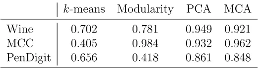
6.2.2 Results . . . 70
Chapter 7 Conclusion . . . 79
7.1 Contributions . . . 80
7.2 Future Research . . . 80
LIST OF TABLES
LIST OF FIGURES
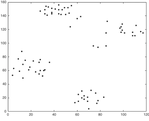
Figure 1.1 Ruspini Dataset. . . 7
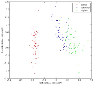
Figure 2.1 A 2-dimensional representation of the iris data given by PCA. . . 18
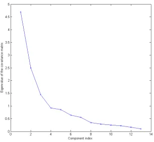
Figure 2.2 Scree graph for the covariance matrix: wine data. . . 23
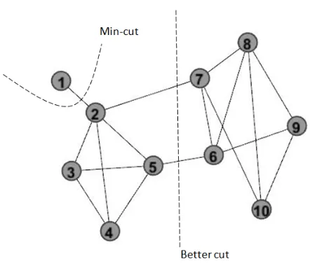
Figure 2.3 A case where minimum cut gives an unsatisfactory partition. . . 27
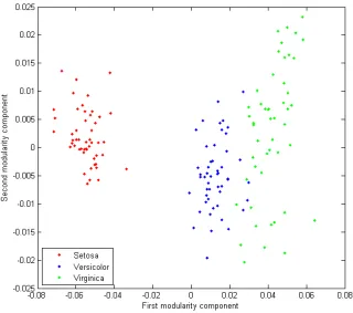
Figure 5.1 A 2-dimensional representation of the iris data given by MCA. . . 64
Figure 6.1 Scree plot of the wine data (centered and normalized) given by PCA. 73 Figure 6.2 Scree plot of the wine data (normalized) given by MCA. . . 73
Figure 6.3 A 2-dimensional representation of the projection of the wine data onto the span of the first two principal components. . . 74
Figure 6.4 A 2-dimensional representation of the projection of the wine data onto the span of the first two modularity components. . . 74
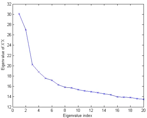
Figure 6.5 Scree plot of the MCC data (centered and normalized) given by PCA. First 20 components included. . . 75
Figure 6.6 Scree plot of the MCC data (normalized) given by MCA. First 20 components included. . . 75
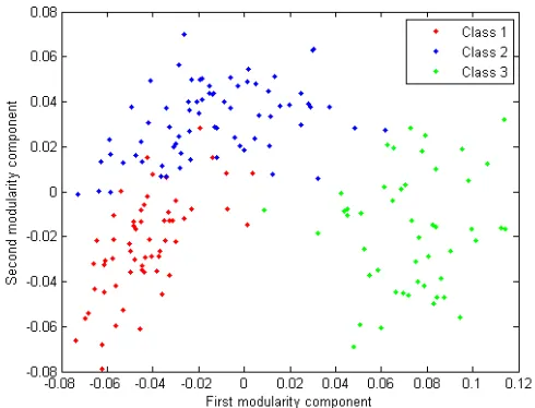
Figure 6.7 A 2-dimensional representation of the projection of the MCC data onto the span of the first two principal components. . . 76
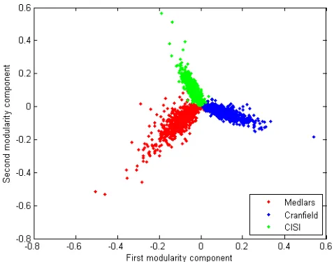
Figure 6.8 A 2-dimensional representation of the projection of the MCC data onto the span of the first two modularity components. . . 76
Figure 6.9 Scree plot of the PenDigit data (centered and unnormalized) given by PCA. First 20 components included. . . 77
Figure 6.10 Scree plot of the PenDigit data (unnormalized) given by MCA. First 20 components included. . . 77
Figure 6.11 A 2-dimensional representation of the projection of the PenDigit data onto the span of the first two principal components. . . 78
CHAPTER
1
Introduction
can perform dimension reduction is more favorited since most of the information in the original data will be kept in the results, and the number of dimensions are greatly reduced so the data can be easily described and stored.
In this paper a novel data analysis method that can help to reveal the cluster structures in the data as well as to perform dimension reduction will be introduced. In Chapter 2 and Chapter 3 some important data analysis methods in the literature will be discussed. In Chapter 4 we will give the definition to the modularity components, and in Chapter 5 some important properties of the modularity components will be stated and proven. Chapter 6 contains some experimental results and Chapter 7 is the conclusion.
1.1
Cluster Analysis
In the next section we will talk more about data.
1.2
About Data
1.2.1
Attributes
A data set usually contains some attributes and data points. Attributes are used to describe some basic characteristics of the data points. In [75], attributes are classified into four types:
1. Nominal: Variables that are used to distinguish different objects. The information given by nominal variables cannot be used to order objects. Examples: gender, zip codes, travel destinations.
2. Ordinal: Variables that provide information to order objects, but the differences between values have no meanings. Examples: Level of education, street numbers. 3. Interval: Variables that provide information to order objects, and the differences
between values have some meaning, but the ratios between values have no meanings. For example, calendar dates is a interval attribute. There are three days strictly between July 1st, 2015 and July 5th, 2015, but the ratio between the two end dates has no meaning.
4. Ratio: Variables that both differences and ratios between different values have meanings. For example, age is a ratio attribute. A 40-year-old man is twenty years older than a 20-year-old woman, and is twice as old as the woman.
the attributes are numeric. It is also noticeable that since the attributes are used to describe the characteristics of the data, it is possible that different attributes have different units and scales. In these cases sometimes it is necessary to normalize the attributes to make them having the same scale to extract useful information. More discussions about normalizing attributes will be given in Chapter 2.
1.2.2
Data Quality
Before applying clustering analysis, it is more desirable to get familiar with the data and perform some preprocessing if necessary. It is quite often that the data contains some noise, outliers or missing values, and the data analysis tools may be sensitive to them. For instance, principle component analysis (PCA) is a very popular data analysis method. The method can give cluster structure of the data while reducing the number of dimensions, and is widely used in image and motion processing [58, 61, 78]. However, it is mentioned in [14] and [33] that it is very sensitive to the outliers. In order to get more reliable clustering results, outlier detection algorithms may be applied before cluster analysis. So before using PCA some outlier detection methods may be applied. Here we list some data quality issues that data analysts may pay attention to. Hodge [31] gives a nice survey about outlier detection methods.
independent and identically distributed (also known as i.i.d.). In this paper, it will be assumed that the noise is distributed independently and identically.
2. Outliers: Outliers are the data points that are different from most of other data. Like PCA, some data analysis algorithms are sensitive to the outliers, so it may be necessary to detect the outliers in the preprocessing step. Such techniques are also called anomaly detection. Support vector data description (SVDD) [76] is one of the anomaly detection methods. The basic idea of SVDD is to draw a “circle” based on the known information in the training step, and use the circle to identify the outliers in the testing step. More methods about anomaly detection can be found in [75].
3. Missing values: Missing value occurs when there is no information provided for a data point in some feature. For example, the rating of a movie given by a user may be missing just because the user has not watched the movie. The missing values can be eliminated, estimated or ignored with some advantages or disadvantages. In this paper, it will be assumed that the missing values, if they exist, are properly handled so they will not get in our way.
1.3
Practical Questions about Cluster Analysis
1.3.1
How to Get Better Clustering Results?
Theorem 1.1 (The Fundamental Theorem of Cluster Analysis). There does not exist a best method, that is, one which is superior to all other methods, for solving all problems
in a given class of problems.
A realistic problem we have to face is that different clustering algorithms performed on the same data may give different clustering results because they use the same information differently. Even the same clustering algorithm applied on the same data may give different results due to different initial points given to the algorithm. This disagreement from the algorithms may bring confusion and difficulty in selecting proper algorithms to analyze the data. A promising solution to this problem is the idea of consensus clustering [59, 57, 67]. The basic idea of consensus clustering is that, if two objects are supposed to be in the same cluster, then the majority of the algorithms should agree to group them together. On the other hand, if two objects are supposed to be separated to different clusters, then the majority of the algorithms should agree to separate them. One example of consensus clustering is introduced in [84]. In the paper different clustering algorithms are run with different initial settings and number of clusters. An adjacency matrix is built for each run to represent if two data points are put in the same cluster or not, and then the sum of all adjacency matrices are calculated for further analysis.
1.3.2
How Many Clusters?
clusters. The method of using plots of sum of squared error (SSE) or silhouette coefficient versus the number of clusters is introduced in [75]. Meyer and Wessell use the number of eigenvalues in the Perron Cluster discussed in [15] and [16]. Race [66] uses the consensus clustering technique to determine the number of clusters. In this paper we will focus on building the modularity components and discussing their properties, so we will just assume in this paper that the number of clusters is already given to us.
1.4
Notations
In this paper a lot of mathematical notations will be used. To avoid confusions, here the notations that will be used in this paper will be listed.
1. Capital bold-faced letters (A, B, X, etc.) denote matrices.
2. Lower cased bold-faced letters (u, v, b, etc.) denote vectors.
3. Single subscripts (vi) of a vector denote the index of a column in a matrix or an eigenvector of a matrix.
4. Greek letters (α, β,λ, etc.) denote the eigenvalues of matrices. Single subscripts of Greek letters (λi) denote the indices of eigenvalues of a matrix.
5. Double subscripts (Aij) denote the row and column indices of an entry in a matrix unless with some other explanations.
6. e denotes a vector with all 1’s with proper size.
CHAPTER
2
Background and Literature Review
In this chapter we will look at some data analysis methods that can help to reveal the cluster structures in the literature.
2.1
K
-means
K-means is a clustering method aims to partition the data points x1,x2, · · ·, xn intok clusters such that each data point belongs to the cluster that has the nearest mean. The means are also called the centroids, and act as the prototypes of the clusters [75]. The term “k-means” was first used in MacQueen’s paper [52], although the idea was already used in Steinhaus’s paper [73]. The basic algorithm of k-means was proposed by Lloyd [50] and Forgy [25].
of squared error:
SSE = k X
i=1 X
xj∈Ci
kxj −cik22, (2.1)
where the Ci’s are the clusters and the ci’s are the centroids of the clusters. It is proved in [75] that the centroids minimizes Eq. 2.1 are the means:
ci = 1 mi
X
xj∈Ci
xj. (2.2)
The algorithm of k-means is presented in Algorithm 1.
Algorithm 1 Euclidian k-means
Require: Data pointsx1,x2, · · ·, xn, initial centroids c1, c2,· · ·, ck. • repeat
Assign each data point to the cluster with nearest centroid with Euclidean distance.
Calculate the new centroids with Eq. 2.2. • until The centroids do not change.
return Clusters C1, C2,· · ·, Ck.
step [75].
2.2
Principal Component Analysis
It is not rare for real world data to have variables correlated with each other. When the number of variables is more than needed, then feature selection or extraction methods may be necessary. In this case a good clustering algorithm should be able to achieve the following goals:
1. To reveal the cluster structures in the data;
2. To reduce the dimension in the data;
3. To keep as much as possible the useful information in the original data.
The modularity component analysis method we are going to introduce in this paper and the principal component analysis method can both achieve these goals. PCA is first introduced by Pearson [65] and Hotelling [32], while the singular vector decomposition, which underlies PCA, is already discussed in [3] and [42]. Jolliffe’s book [40] has more discussions and applications about PCA.
2.2.1
Definition of Principal Components
Each data point has a score on each of the components based on how the data is “related with” the component. The principal component analysis can be understood as changing a basis from the elementary basis {e1,e2,· · · ,ep} to a new basis {u1,u2,· · · ,up}, and the scores are the new coordinates of the data points in the new coordinate system. To give a mathematical definition of the principal components, suppose we have a p×n data matrix X0 wherep is the number of variables and n is the number of data points. We want to find a vector u1 such that ku1k2 = 1 and the sample variance of the vector
uT1X0 =
uT
1x1 uT1x2 · · · uT1xn
is maximized. The word “sample” means we are dealing with data rather than random variables, and will be omitted in the later discussion for the sake of simplicity. If the mean vector of the xi’s is x, then the problem becomes of solving
max
ku1k2=1
1 n−1
n X
i=1
(uT1(xi−x))2. (2.3)
Subtracting the mean vector from each data point vector is also calledcentering. Eq. 2.3 can be formulated as
max
ku1k2=1
uT1Su1, (2.4)
where
Sp×p = 1 n−1
n X
i=1
(xi−x)(xi−x)T (2.5)
is the covariance matrix of the data. It can be also written in the matrix form:
S= 1
n−1XX T
where
X =
x1−x x2−x · · · xn−x
(2.7)
represents the centered data. The Rayleigh-Ritz Theorem [51] says the solution to Eq. 2.4 is given by the eigenvector corresponding to the largest eigenvalue λ1 of S, and the maximum value of Eq. 2.5 is given byλ1. That means λ1 is the largest variance in the centered data. The i-th principal components where i≥2 is the solution to the problem
max
kuik2=1
ui⊥uj,j=1,···,i−1
uTi Sui, (2.8)
and by the Rayleigh-Ritz Theorem ui is the eigenvector corresponding to thei-th largest eigenvalueλi of S, and the maximum value of Eq. 2.8 is given byλi. That means λi is the largest variance in the centered data that is uncorrelated with the preceding principal components. Since the eigenvectors ofS andXXT are the same, and the eigenvalues of S
are 1/(n−1) proportional to the eigenvalues of XXT, the principal components can be also computed from XXT, or singular vectors of X.
is set to 10000. With the variables normalized, the covariance matrix is
S1 =
1.0000 −0.1176 0.8718 0.8179
−0.1176 1.0000 −0.4284 −0.3661 0.8718 −0.4284 1.0000 0.9629 0.8179 −0.3661 0.9629 1.0000
,
and the first principal component is
u1 = 0.5211 −0.2693 0.5804 0.5649 .
The covariance matrix of the unnormalized data is
S01 =
1.0000 −0.1176 0.8718 81.7941
−0.1176 1.0000 −0.4284 −36.6126 0.8718 −0.4284 1.0000 96.2865 81.7941 −36.6126 96.2865 10,000
,
and the first principal component is
It can be seen that in the unnormalized case, the direction of the first principal component is almost identical to e4, and that means the data is described mostly by the fourth variable, which is misleading. Therefore, when the data has different scales it is often necessary to normalize the variables after centering. In the following discussion in this section, it will be assumed that the data has been centered and normalized.
2.2.2
Singular Value Decomposition and Scoring the Data
The singular value decomposition (SVD) technique is a matrix factorization method and plays a very important role in PCA. Here we write down the definition of SVD in [56]:Definition 2.1. For each A ∈ Rm×n of rank r, there are orthogonal matrices U m×m,
Vn×n and a diagonal matrix Dr×r =diag(σ1, σ2,· · · , σr) such that
A=U
D 0 0 0
m×n
V with σ1 ≥σ2 ≥ · · · ≥σr≥0. (2.9)
The σi’s are called the nonzero singular values of A. When r < p= min{m, n}, A is
said to have p−r additional zero singular values. The factorization in Eq. 2.9 is called
a singular value decomposition of A, and the columns in U and V are called the
left-hand and right-hand singular vectors for A, respectively.
The SVD is related with PCA in two ways. First, the principal components we defined in Section 2.2.1 can be derived from SVD. To see this, suppose Xp×n is the data matrix after centering and normalization. Let the SVD of X to be
X=UΣVT =U
Then the matrix XXT can be written as
XXT =U
D2 0
0 0
p×p
UT. (2.11)
Therefore, the eigenvalues of XXT are the squares of the singular values of X, and the eigenvectors of XXT are the left-hand singular values ofX. To calculate the eigenvalues and eigenvectors of XXT, it is sufficient to apply SVD on X.
Second, SVD is related to the scores of the data on the principal components. The inner product uT
jxi is the projection of xi onto the span of uj and is also called the score of the i-th data point on the j-th principal component [40]. From X=UΣVT we have
UTX=ΣVT = uT
1x1 uT1x2 · · · uT1xn
uT2x1 uT2x2 · · · uT2xn ..
. . .. ...
uTpx1 uTpx2 · · · uTpxn , (2.12)
which contains the scores of each data point on each principal component. Therefore, the
score matrix UTX can be computed with ΣVT. An advantage of using ΣVT to compute the score matrix is the Σ is very sparse and the computations can be very efficient.
2.2.3
Dimension Reduction, Low Rank Representation of Data
and Clustering
each component, and is just the trace of the covariance matrix S. Since the trace of a matrix is equal to the sum of its eigenvalues, it can be computed that how much variance is kept by the firstk principal components:
Variance retained, Vk= Pk
i=1λi
trace(S). (2.13)
Therefore, if the sum of the first k eigenvalues of the covariance matrix can take a large portion of the total sum of all eigenvalues, then the first k principal components retain the majority of the variance in the data. The score matrix
Tk =UTkX=
uT1
uT2
.. . uT k X (2.14)
2.2.4
Summary of Properties of Principal Components
Now we summarize the important properties of the principal components. We will first describe the properties, then state the properties again by writing them as theorems. To make the points more clear, it will be assumed that the data matrix X has full row rank.
• The principal components are orthogonal to each other.
• If we project the data onto the span of a principal component, we get a scalar multiple of the score vector that can reveal the cluster structure in the data based on the signs of the entries in the score vector.
• The first principal component has the largest variance of the data. Each succeeding principal component has the largest variance with the constraint that it is orthogonal to all previous principal components.
Next we state the properties as theorems. Let the ui’s be the principal components.
Theorem 2.2. For 1≤i, j ≤p, we have
uTi uj =
1 i=j, 0 i6=j.
(2.15)
Proof. By definition.
Theorem 2.3. Let Pui be the projector onto the span of ui. Then we have
PuiX=σiuiv
T
i , (2.16)
Proof. LetX =UΣVT be the SVD of X.
PuiX =uiu
T
i X=ui
uTi x1 uTi x2 · · · uTixn
=ui
ΣVT
i∗
=σiuivTi .
Theorem 2.4. Letσi be the i-th largest singular value of X. Moreover, for 2≤i≤p, let
Xi =X− i−1 X
j=1
uiuTi X, (2.17)
then σ2i is the largest eigenvalue of XiXiT, and ui is the corresponding eigenvector of σ2i.
Proof. By the discussion in Section 2.2.1.
Algorithm 2 Clustering with Principal Component Analysis
Require: Ap×n data matrixX0, number of clustersk, number of principal components t.
• Center and normalize X0 to matrixX.
• Compute the SVD of X with Eq. 2.10.
• Let the score matrix Tt be the first t rows of the matrix ΣVT.
• Let pi be the i-th colomn of Tt.
• Cluster the pi’s with k-means into clustersC1, C2, · · ·, Ck.
return Clusters G1,G2, · · ·, Gk such that Gi ={j|pj ∈Ci}.
2.2.5
How Many Principal Components?
From the discussion above it can be seen that PCA is hoped to perform dimension reduction while retain as much as possible the variance in the original data and keep the cluster structure. Then there is a natural but essential question: How many principal components should be used to achieve these goals? A true but diplomatic answer is “It depends on the data”. Accepting this answer but being a little bit arbitrary, we seek for some rules and research papers that may help to get a proper number of principal components, rather than trying numbers from one to p.
criterion based onVk.
The second method is just set a threshold on the λk in Eq. 2.13. Kaiser’s rule says that only the λk’s that exceed 1 and their corresponding principal components should be retained. Jolliffe [41] argues that setting λk = 1 to be the threshold may discard too much useful information, and 0.7 may be a better threshold.
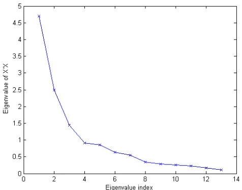
The third method is to plot the λk’s against the k to get a scree graph [11]. Figure 2.2 is an example of a scree graph. People may calculate
bk =
λk−1 −λk λk−λk+1
, 1< k < p−1 (2.18)
to get the k∗ that has the maximal bk (also called the “elbow”), and drop the λk’s that are smaller than k∗. For the wine data [49] that has the scree plot in Figure 2.2, the elbow rule suggests to keep the first four principal components.
There are other techniques that can be applied to determine how many principal compo-nents to keep. Statistical methods are studied in [2, 35, 77, 5, 4]. These research focused on using hypothesis tests to determine how many principal component are statistical significant. Wold [86], Eastment and Krzanowski [19], and Krzanowski and Kline [45] studied the residual between the original data and the low-rank estimation of the data given by SVD. The principal components would be dropped if adding it causes no signifi-cant decrease to the residual. There are also some papers comparing these methods, such as [69, 27, 20].
2.2.6
Other Research about Principal Components
It is mainly used to cluster web pages, and iteratively uses the first principal component to bipartition the data. Boley [7] continued this research and proposed the principal direction divisive partitioning algorithm (PDDP). Candes et al. [10] and Wright et al. [87] considered a way to recover a low-rank representation of the data when the data is corrupted. Wang et al. [82] and Jeng [37] discussed a moving window PCA method that can be used on time series.
2.3
Spectral Clustering
The spectral clustering method is one of the most widely used techniques for graph partitioning. The theory is based on Miroslav Fiedler’s research [21, 22, 23]. In this section we will first introduce the classical spectral clustering algorithm, and then some extended versions of spectral clustering will be discussed.
2.3.1
Classical Spectral Clustering
We start with a graphG(V, E) withV the set of vertices andEthe set of edges. We assume that the graph G is weighted and undirected, so its adjacency matrix A is symmetric. The (i, j)-th entry of A is the weight on the edge between verticesiandj, or zero if there is no edge between them. The graph is connected if there is a path between every pair of vertices in the graph. A connected component is a maximal connected subgraph of G. Suppose|V|=n and |E|=m, then the degree of vertex i is defined by the sum of weights on the edges connected with i, i.e.
di = n X
i=1
It can be seen that di is also the i-th row sum of A. The degree matrix D is a diagonal matrix with di on its i-th diagonal entry. Now we give the definition of the Laplacian matrix.
Definition 2.5. The Laplacian matrix L of a weighted and undirected graph is defined as
L=D−A. (2.20)
The Laplacian matrix is symmetric and positive semi-definite. The smallest eigenvalue of L is zero, and its corresponding eigenvector is the vectore. For any vector v∈Rn, we have [79]
vTLv= 1 2
n X
i,j=1
aij(vi−vj)2. (2.21)
If the graph is not connected, then the number of connected components in the graph is equal to the algebraic multiplicity of the zero eigenvalue of L. To see this, note that the Laplacian matrix of a graph that contains k connected components has the form
L= L1 L2 . .. Lk ,
in total. If the graph is connected, then consider the matrix
M=A−D+dmaxI=dmaxI−L, (2.22)
where dmax = max{d1, d2,· · · , dn}. Then M is nonnegative and irreducible. From the Perron-Frobenius theorem [56], the largest eigenvalue of M is simple. Also notice that there is a relation between the eigenvalues ofM and the eigenvalues of L:
λi(L) = dmax−λi(M), (2.23)
therefore the smallest eigenvalue of L is simple.
In [21], Fiedler defined the second smallest eigenvalue of the Laplacian matrix, λ2, as the
algebraic connectivity of the graph. The eigenvector of L corresponding to λ2 is called the Fiedler vector. In [22], Fiedler proved that if a connected graph is partitioned by the signs of the Fiedler vector (an arbitrary decision has to be make if some entries are zero), then the two subgraphs are also connected. If the desired number of clusters k is given, then by recursively bipartition the graph with Fiedler vectors, k connected subgraphs of G can be achieved.
2.3.2
Graph Cuts and Spectral Clustering
G2, · · ·,Gk, such that
cut(G1, G2,· · · , Gk) = 1 2
k X
i=1
W(Gi, Gi), (2.24)
is minimized, where
W(A, B) = X i∈A,j∈B
aij (2.25)
and Gi is the complement of Gi. The meaning of Eq. 2.24 is to cut the graph such that minimized number of edges are cut in the process. Although intuitive, in practice the solution to this problem is often helpless, because in many cases the solution put a single vertex into one group and all other vertices in another group. One way to avoid getting this kind of unsatisfactory results is to try to cut the graph while keeping the sizes of the clusters more balanced. Two examples of such cutting techniques are solving the
RatioCut and Normalized Cut problems.
RatioCut
Now we give another way to cut the graph called the RatioCut [30]:
Definition 2.6. Suppose G1, G2, · · ·, Gk is a partition of G. The RatioCut is defined by
RatioCut(G1, G2,· · · , Gk) = 1 2
k X
i=1
W(Gi, Gi)
|Gi| =
k X
i=1
cut(Gi, Gi)
|Gi|
, (2.26)
where |G| is the number of vertices in G.
Suppose a set of k indicator vectors vi is defined by
vij = 1 √
|Gj| if nodei in Gj
0 otherwise.
(2.27)
Then it can be seen that the vi’s are orthonormal to each other. If the columns of the matrix V ∈Rn×k are thev
i’s, thenVTV=I. In [79], it is proven that minimizing the RatioCut is equivalent to minimizing the trace of the matrix VTLV. However, solving the equation with the constraint to the form of V is NP-hard. Then the constraint to
V is relaxed by allowing the entries inV to take any real values. The relaxed problem becomes solving
min
V∈Rn×k
Tr(VTLV) subject to VTV =I. (2.28)
Algorithm 3 Unnormalized Spectral Clustering [79]
Require: Ann×n adjacency or similarity matrix A, number of clusters k. • Compute the Laplacian matrix L=D−A.
• Compute the smallest k eigenvalues of L and their corresponding eigenvectors.
• Form the matrix V with the k eigenvectors of L as columns.
• Let pi be the i-th row of V.
• Cluster the pi’s withk-means into clusters C1, C2, · · ·, Ck.
return Clusters G1,G2, · · ·, Gk such that Gi ={j|pj ∈Ci}.
As an example to illustrate how to use Fiedler vector to partition a graph, we use Algorithm 3 to partition the graph in Figure 2.3. The adjacency matrix of the graph is
A =
0 1 0 0 0 0 0 0 0 0 1 0 1 1 1 0 1 0 0 0 0 1 0 1 1 0 0 0 0 0 0 1 1 0 1 0 0 0 0 0 0 1 1 1 0 1 0 0 0 0 0 0 0 0 1 0 1 1 1 0 0 1 0 0 0 1 0 1 0 1 0 0 0 0 0 1 1 0 1 1 0 0 0 0 0 1 0 1 0 1 0 0 0 0 0 0 1 1 1 0
and the Laplacian matrix is L=
1 −1 0 0 0 0 0 0 0 0
−1 5 −1 −1 −1 0 −1 0 0 0
0 −1 3 −1 −1 0 0 0 0 0
0 −1 −1 3 −1 0 0 0 0 0
0 −1 −1 −1 4 −1 0 0 0 0
0 0 0 0 −1 4 −1 −1 −1 0
0 −1 0 0 0 −1 4 −1 0 −1
0 0 0 0 0 −1 −1 4 −1 −1
0 0 0 0 0 −1 0 −1 3 −1
0 0 0 0 0 0 −1 −1 −1 3
.
Then the Fiedler vector, i.e. the eigenvector corresponding to the second smallest eigenvalue, is
By looking at the signs of the entries inv2, we put the first five vertices into one group, and the last five vertices into the other group.
Normalized Cut
There is another kind of spectral clustering technique that aims to minimize the objective function called Normalized Cut, or NCut introduced by Shi and Malik [72]:
Definition 2.7. Suppose G1, G2, · · ·, Gk is a partition of G. The NCut is defined by
NCut(G1, G2,· · · , Gk) = 1 2
k X
i=1
W(Gi, Gi)
vol(Gi) =
k X
i=1
cut(Gi, Gi)
vol(Gi)
, (2.29)
where
vol(G) = X i∈G
di. (2.30)
It can be seen that the technique used in solving the NCut problem is quite similar to the case of solving the RatioCut problem. Suppose a set of k indicator vectors vi is defined by
vij = 1 √
vol(Gi)
if nodei inGj 0 otherwise.
(2.31)
Then the vi’s are orthonormal to each other. If the columns of the matrix V ∈Rn×k are the vi’s, then VTDV =I. In [79], it is proven that minimizing the NCut is equivalent to minimizing
min
V Tr(V
TLV) subject to VTDV=I. (2.32)
substitute V byD−1/2T, where T∈
Rn×k. The relaxed problem becomes solving
min
T∈Rn×kTr(T
TD−1 2LD−
1
2T) subject to TTT=I. (2.33)
By the Rayleigh-Ritz theorem again, the columns of T are formed by the eigenvectors corresponding to the first k smallest eigenvalues of
Lsym=D−
1 2LD−
1
2. (2.34)
Solving back for V with V =D−1/2T, it can be seen that the columns of V are the the eigenvectors corresponding to the first k smallest eigenvalues of
Lrw =D−1L. (2.35)
Algorithm 4 Normalized Spectral Clustering by Shi and Malik [72]
Require: Ann×n adjacency or similarity matrix A, number of clusters k. • Compute the Laplacian matrix L=D−A.
• Compute the Normalized Laplacian matrix Lrw =D−1L.
• Compute the smallest k eigenvalues of Lrw and their corresponding eigenvectors.
• Form the matrix V with the k eigenvectors of Lrw as columns.
• Let pi be the i-th row of V.
• Cluster the pi’s withk-means into clusters C1, C2, · · ·, Ck.
return Clusters G1,G2, · · ·, Gk such that Gi ={j|pj ∈Ci}.
Other Spectral Clustering Algorithms and Discussions
Algorithm 5 Normalized Spectral Clustering by Ng, Jordan and Weiss [64]
Require: Ann×n adjacency or similarity matrix A, number of clusters k. • Compute the Laplacian matrix L=D−A.
• Compute the Normalized Laplacian matrix Lsym =D−
1 2LD−
1 2.
• Compute the smallest k eigenvalues of Lsym and their corresponding eigenvectors.
• Form the matrix V with the k eigenvectors of Lsym as columns.
• Normalize each row of V to form a matrix U. • Let pi be the i-th row of U.
• Cluster the pi’s withk-means into clusters C1, C2, · · ·, Ck.
return Clusters G1,G2, · · ·, Gk such that Gi ={j|pj ∈Ci}.
Other than using the eigenvectors of a different Laplacian matrix, Algorithm 8 nor-malizes each row of the V matrix. One reason of doing this, as pointed in [79], is because the eigenvector corresponding to the smallest eigenvalue of Lsym is D1/2e instead of e. In the indicator matrices in Eq. 2.27 and Eq. 2.31 for the ideal cases, there is one and only one nonzero entry in each row. In the solutions to the relaxed problems (Eq. 2.28 and Eq. 2.33), it can be guaranteed that for each row of the matrix V there is at least one entry that has value (1/√n)e, since e is the eigenvector corresponding to the zero eigenvalue of L and Lrw. So each row in the V matrix is “bounded away” from zero. However, if a vertex in the graph has very small degree, then it is possible that in the V
each row in V, it can be guaranteed that each row is not close to the origin.
CHAPTER
3
Modularity Graph Partitioning
The data analysis method introduced in this paper is based on the modularity graph partitioning method introduced by Norman and Girvan in [63], and further explained by Newman in [62]. In this chapter we will define the modularity matrix and discuss how to use the modularity matrix to partition a graph. We will also discuss some other research about modularity partitioning.
3.1
The Modularity Matrix
We start with the definition of the modularity matrices.
given. Then the modularity matrix corresponding to the graph is defined by
B=A−dd
T
2m , (3.1)
where m is the number of edges in the graph and
d=
d1 d2 · · · dn T
(3.2)
is the degree vector.
In Definition 3.1, the (i, j)-th entry in the rank-one matrix (ddT)/(2m) represents the expected number of edges between nodes i and j in a graph having random edges where the degrees of the nodesi and j aredi anddj, respectively. So the meaning of the matrix
B is the comparison between the given graph and the graph that contains the expected number of edges. If two nodes should be put in the same cluster, then the number of edges between these nodes in the actual graph should be more than the expected number of edges, and the corresponding entry in the modularity matrix should be positive. On the other hand, if two nodes should be put in different clusters, then the number of edges between these nodes in the actual graph should be less than the expected number of edges, and the corresponding entry in the modularity matrix should be negative.
Here are some basic properties of the modularity matrix:
1. A modularity matrix is symmetric and all of its eigenvalues are real;
2. A modularity matrix has an eigenpair (0,e);
In the following sections we will discuss how to use the modularity matrix to partition a graph.
3.2
Bipartitioning a Graph
Suppose we are given a weighted, undirected graph, so its adjacency matrixA is known. Then for a particular bipartition (G1, G2) of the graph, we can express the partition with a vector s by letting
si =
1 if node i in G1
−1 otherwise.
(3.3)
Then we can define the modularity corresponding the graph with the given bipartition.
Definition 3.2. Given a graph with a bipartition s, the modularity of the graph
corre-sponding to the bipartition is defined by
Q(s) = 1 4ms
T
Bs. (3.4)
For a given graph, since its number of edges is constant, the definition of modularity can be also written as
Q(s) = sTBs. (3.5)
It can also be written in the summation form
Q(s) = X 1≤i,j≤n
sisjBij. (3.6)
the expected number of edges. Therefore we may have four cases for the term sisjBij:
1. If si and sj have the same sign, which means in the given partition the two nodes are grouped together, and at the same timeBij is positive, which means the number of edges in the actual graph is more than expected, then the term sisjBij will be positive.
2. If si and sj have different signs, which means in the given partition the two nodes are grouped in different clusters, and at the same time Bij is negative, which means the number of edges in the actual graph is less than expected, then the term sisjBij will also be positive.
3. If si and sj have the same sign, and Bij is negative, thensisjBij will be negative.
4. If si and sj have different signs, and Bij is positive, then sisjBij will be negative.
From these four cases it can be seen that Q(s) is positive when the signs of Bij and sisj are the same, and negative when the signs are different. This property can be understood as the “correctness” of grouping nodes i andj together. To be more clear, Q(s) increases when the partition make the “correct” decisions, and decreases when the “wrong” decisions are made. Therefore, the goal of modularity graph partitioning is to find such a vector
s that subject to Eq. 3.3 to maximize Q(s). However, the problem is NP-hard due to the special restriction on the vector s. Newman [62] relaxed the problem by allowing the entries in s to be any arbitrary real values, and the graph will be partitioned based on the signs of the entries in the vector s. It is easy to see that the dominant eigenvector of
B can solve the relaxed problem.
zero. Newman [62] discussed this case. Since the eigenvector corresponding to the zero eigenvalue is the e vector, the largest eigenvalue is zero indicates thatall vertices in the graph should be put into the same cluster. That means there is only one cluster in the graph. No partitioning should be done in this case.
To generate more than two subgraphs, the partitioning method discussed above wil be applied several times to build a hierarchy until the desired number of clustersk is reached. Each time the subgraph that can contribute more modularity while being partitioned. Next we give the algorithm for modularity clustering.
Algorithm 6 Modularity Clustering by Newman [62]
Require: Ann×n adjacency or similarity matrix A, number of clusters k. • repeat
Compute the modularity matrix B with Eq. 3.1. Compute the largest eigenvalue λ1 of B.
If λ1 = 0 then return the whole data as one cluster. If λ1 >0 then compute its corresponding eigenvector v1.
Cluster the entries inv1 by their signs to get clusters C1 and C2.
Bipartition the graph to get subgraphs G1 andG2 such thatGi ={j|v1j ∈Ci}. Pick the subgraph with largerQ(s) in Eq. 3.4
• until The number of desired number of clusters is reached or no positive eigen-values can be found for the modularity matrices of the subgraphs. Suppose in the latter case there are k0 subgraphs.
When the modularity clustering algorithm is applied on the toy example in Figure 2.3, the dominant eigenvector of the modularity matrix is
v1 = −0.1252 −0.3479 −0.3708 −0.3708 −0.3116 0.2276 0.2173 0.3991 0.3425 0.3398 ,
which indicates that the first five vertices should be put into the one group and the last five vertices into the the other group.
and compute the eigenvectors once. However, the question is why the eigenvectors other than the dominant eigenvector of theB matrix can give us the information of the clusters. Those eigenvectors may only contain irrelevant information or just noise in the data. If the eigenvectors contain useful information, then should we keep all of them? If there is an order of “importance” for the eigenvectors, then how the order is defined and how to order the eigenvectors? These questions need to be answered before just taking several eigenvectors and partition the graph.
3.3
Other Discussions about Modularity Clustering
The questions raised in the last section will be answered in the following chapters. Before diving into the discussion we first look at some other discussions about modularity clustering in the literature. The modularity partitioning algorithm has been widely applied and discussed since proposed by Newman and Girvan [63]. For instance, it has been applied to reveal human brain functional networks [55] and ecological networks [26], and used in image processing [54]. Blondel et al. [6] proposed a heuristic that can reveal the community structure for large networks. Rotta and Noack [70] compared several heuristics in maximizing modularity. DasGupta and Desai [13] studied the complexity of modularity clustering. The limitations of the modularity maximization technique are discussed in [29] and [46]. Bolla [8] normalized the modularity matrix to form
Bsym=D−
1 2BD−
1
just like the way Lsym is formed in Eq. 2.34. Zhang and Zhao [89] normalized the modularity matrix in another way to form
Brw =D−1B, (3.8)
as the way Lrw is formed in Eq. 2.35. To make the discussion more complete, here we write down the normalized modularity clustering algorithms:
Algorithm 7 Normalized Modularity Clustering by Bolla [8]
Require: Ann×n adjacency or similarity matrix A, number of clusters k. • Compute the modularity matrix B with Eq. 3.1.
• Compute the normalized modularity matrix Bsym =D−
1 2BD−
1 2.
• Compute the largest k eigenvalues of Bsym and their corresponding eigenvectors.
• Form the matrix V with the k eigenvectors of Bsym as columns.
• Let pi be the i-th row of V.
• Cluster the pi’s withk-means into clusters C1, C2, · · ·, Ck.
Algorithm 8 Normalized Modularity Clustering by Zhang and Zhao [89]
Require: Ann×n adjacency or similarity matrix A, number of clusters k. • Compute the modularity matrix B with Eq. 3.1.
• Compute the Normalized Laplacian matrix Brw =D−1B.
• Compute the smallest k eigenvalues of Brw and their corresponding eigenvectors.
• Form the matrix V with the k eigenvectors of Brw as columns.
• Let pi be the i-th row of V.
• Cluster the pi’s withk-means into clusters C1, C2, · · ·, Ck.
return Clusters G1,G2, · · ·, Gk such that Gi ={j|pj ∈Ci}.
CHAPTER
4
Definition of Modularity Components
4.1
Eigenvalues and Eigenvectors of DPR1 Matrices
Suppose the SVD of the uncentered data matrixXisX=UΣVT and there arek nonzero singular values. Then the similarity matrix
A=XTX=VΣTΣVT (4.1)
hask positive eigenvalues. From the interlacing theorem mentioned in [9] and [85], it is guaranteed that the largest k−1 eigenvalues of the modularity matrix
B=A− dd
T 2m =X
TX− ddT
2m (4.2)
are positive. If the k dominant eigenvalues of A are simple, then the eigenvectors of B
corresponding to the largest k−1 eigenvalues can be written as linear combinations of the eigenvectors of A. The proof of the lemma is based on a theorem from [9] about the interlacing property of a diagonal matrix and its rank-one modification and how to calculate the eigenvectors of a DPR1 matrix [56]. The theorem can also be found in [85].
Theorem 4.1. LetC=D+ρvvT, whereDis diagonal,kvk
2 = 1. Letd1 ≤d2 ≤ · · · ≤dn
be the eigenvalues of D, and let d˜1 ≤ d˜2 ≤ · · · ≤ d˜n be the eigenvalues of C. Then ˜
d1 ≤d1 ≤d˜2 ≤d2 ≤ · · · ≤d˜n ≤dn if ρ <0. If the di are distinct and all the elements of
v are nonzero, then the eigenvalues of C strictly separate those of D.
Corollary 4.2. With the notations in Theorem 4.1, the eigenvector of Ccorresponding
to the eigenvalue d˜i is given by
(D−d˜iI)−1v. (4.3)
the eigenvalues of the original diagonal matrix. In the next section we will use the theorems about the DPR1 matrices to state and prove the lemma that thek−1 dominant eigenvectors of B can be written as a linear combination of the eigenvectors of A.
4.2
Dominant Eigenvectors of Modularity Matrices
In this section we will develop the relation between the dominant eigenvectors of the modularity matrices and the eigenvectors of XTX, or the singular vectors of X. This relation will help us to define the modularity components.
Lemma 4.3. Suppose the largest k−1 eigenvalues of B are β1 > β2 >· · ·> βk−1 and
the nonzero eigenvalues ofA =XTX are α1 > α2 >· · ·> αk. Further suppose that for
1≤i≤k−1we have βi 6= αi and βi 6=αi+1. Then the eigenvectorbi of B can be written
by
bi = k X
j=1
γijvj, (4.4)
where
γij = v
T j d (αj−βi)kdk2
. (4.5)
Proof. If A=XTX, and if the SVD ofX is X=UΣVT, then
A=VΣTΣVT =VΣAVT, (4.6)
where ΣA is an n×n diagonal matrix. Suppose the rows and columns ofA are ordered such that ΣA = diag(α1, α2,· · · , αn), where α1 > α2 >· · ·> αk > αk+1 =· · ·=αn= 0. Let V=
v1 v2 · · · vn
eigenvalues β1 > β2 >· · ·> βk−1. Since B=A−ddT/(2m), we have
B=A− dd
T
2m =VΣAV
T −dd T
2m =V(ΣA+ρyy
T)VT, (4.7)
where y=VTd/kVTdk
2 and ρ=−kVTdk22/(2m). SinceΣA+ρyyT is also symmetric,
it is orthogonally similar to a diagonal matrix. So we have
B=VU0ΣBU0TVT, (4.8)
where U0 is orthogonal and ΣB is diagonal. Since ΣA+ρyyT is a DPR1 matrix, ρ <0
and kyk2 = 1, the interlacing theorem applies to the eigenvalues of A and B. More specifically, we have
αk < βk−1 < αk−1 < βk−2 <· · ·< β2 < α2 < β1 < α1.
The strict inequalities hold because of our assumptions. Let B1 = ΣA +ρyyT. Since B=VB1VT, we have BV=VB1. Suppose (λ,u) is an eigenpair of B1, then
BVu=VB1u=λVu (4.9)
implies that (λ,u) is an eigenpair of B1 if and only if (λ,Vu) is an eigenpair of B. By Corollary 4.2, the eigenvector of B1 corresponding to βi, 1≤i≤k−1 is given by
pi = (ΣA−βiI)−1y= (ΣA−βiI)−1
VTd
kVTdk 2
and hence the eigenvector ofB corresponding to βi, 1≤i≤k−1 is given by
bi =Vpi =V(ΣA−βiI)−1
VTd
kVTdk 2
= 1
kdk2 n X
j=1
vT j d αj−βi
vj. (4.11)
Since d=Ae=VΣAVTe where e is a column vector with all ones, we have
vTjd=vTjVΣAVTe =eTjΣAVTe. (4.12)
Since rank(A) = k, we have vTjd = 0 for j > k. Therefore, the eigenvector of B
corresponding to βi, 1≤i≤k−1 is given by
bi = k X
j=1
γijvj, (4.13)
where
γij =
vT j d (αj−βi)kdk2
. (4.14)
The point of Lemma 4.3 is to realize that the vector bi is a linear combination of the
vi. The next lemma gives the linear expression of the vectors bTi X
† in terms of the u
i, where X† is the Moore-Penrose inverse ofX.
Lemma 4.4. With the assumptions in Lemma 4.3, we have
bTi X† = k X
j=1 γij
σj
uTj, (4.15)
Proof.
bTi X† = k
X
j=1 γijvTj
VӆUT
=
γi1 γi2 · · · γik 0 · · · 0
1×n
Σ†UT
=
γi1
σ1
γi2
σ2 · · ·
γik
σk 0 · · · 0
1×p
UT = k X j=1 γij σju T j.
Lemma 4.4 shows that if bi can be written as a linear combination of the vj, then the vectors bTi X† can be written as a linear combination of the ui. In the next section we give the formal definition of the modularity components.
4.3
Definition of Modularity Components
Based on Lemma 4.3 and Lemma 4.4, we may define a set of vectors that we will call modularity components. We will prove in the next chapter that the modularity components have some properties that are analogous to the ones of principal components.
Definition 4.5. Suppose Xp×n is the data matrix, bi is the eigenvector corresponding to
the i-th largest eigenvalue of B, where
B=XTX− dd
T
Under the assumptions in Lemma 4.3, let
mTi =bTi X†= k X
j=1 γij
σj
uTj. (4.17)
The i-th modularity component is defined to be
ci =
mi
kmik2
. (4.18)
By Lemma 4.3 and Lemma 4.4 it can be seen that as long as the assumptions in Lemma 4.3 are met, the modularity components are well-defined, and the definition of ci is based on the linear combination of bT
i X
† in terms of the u
CHAPTER
5
Properties of Modularity Components
In this chapter we will use the definition of modularity components to prove some important properties of modularity components. The properties of the modularity components will be given, and it will be explained why these properties can help in data clustering and dimension reduction. We will also compare the properties of modularity components with the ones of principal components discussed in Chapter 2. It can be seen that the properties of modularity components are quite similar to some of the properties of principal components.
5.1
Orthogonality of Modularity Components
are orthogonal to each other.
Theorem 5.1. With the assumptions in Lemma 4.3, suppose Xp×n is the unnormalized
data matrix,A =XTX, and B =A−ddT/(2m). Supposeb
i, bj are the eigenvectors of
B corresponding to eigenvalues λi and λj, 1≤i, j ≤k−1, respectively. Then we have
B= (BX†)(BX†)T (5.1)
and
ci ⊥cj (5.2)
for i6=j.
Proof. It is sufficient to prove that mi ⊥mj for i6=j. From A=XTX we have
d=Ae=XTXe, (5.3)
and
2m=dTe=eTXTXe. (5.4)
Therefore,
B =A− dd
T 2m =X
TX− (XTXe)(XTXe)T
eTXTXe =X
TX− XTXeeTXTX
eTXTXe . (5.5)
Since XTXX† =XT is always true, we have
BX†=
XTX− X
TXeeTXTX
eTXTXe
=XTXX†−X
TXeeTXTXX†
eTXTXe =X
T −XTXeeTXT
eTXTXe . (5.6) Consequently,
(BX†)(BX†)T =
XT − X
TXeeTXT
eTXTXe
X− Xee
TXTX
eTXTXe
=XTX− 2X
TXeeTXTX
eTXTXe +
(eTXTXe)XTXeeTXTX (eTXTXe)2
=XTX−X
TXeeTXTX
eTXTXe . (5.7)
Therefore B= (BX†)(BX†)T. Since Bb
i =λibi, Bbj =λjbj, λi 6= 0, λj 6= 0, we have
mTi mj = (bTi X
†
)(bTjX†)T =
1 λi
bTi BX†
1 λj
bTjBX†
T
= 1
λiλj
bTi (BX†)(BX†)Tbj = 1 λiλj
bTi Bbj = 1 λi
bTi bj = 0, (5.8)
so
cTi cj =
mT i mj
kmik2kmjk2
(5.9)
implies ci ⊥cj for i6=j.
5.2
Projection of Data onto the Span of Modularity
Components
In this section we will prove that the projection of the uncentered data onto the span of
ci is a scalar multiple of bi.
Theorem 5.2. With the assumptions in Lemma 4.3, let Pci be the projector onto the
span of ci. Then
PciX=
1
kmik2
cibTi . (5.10)
Proof.
PciX =cic
T i X=
1
kmik2
cimTi UΣV
T = 1
kmik2
ci k X j=1 γij σj
uTj
UΣVT
= 1
kmik2
ci
γi1
σ1
γi2
σ2 · · ·
γik
σk 0 · · · 0
1×p
ΣVT
= 1
kmik2
ci
γi1 γi2 · · · γik 0 · · · 0
1×n
VT
= 1
kmik2
ci k X
j=1
γijvTi = 1
kmik2
cibTi .
5.3
Meaning of Eigenvalues of B and the
Correspond-ing Modularity Components
In this section we will prove that the first modularity component has the largest modularity in the data, and each succeeding modularity component has the largest modularity with the constraint that it is orthogonal to all previous modularity components. We will also how the eigenvalues of the modularity matrix defines the “importance” of each modularity component.
Theorem 5.3. With the assumptions in Lemma 4.3, we have
βi = 1
kmik22
, (5.11)
for 1≤i≤k−1. Moreover, let X1 =X and for 1< i≤k−1,
Xi =X− i−1 X
j=1
cjcTjX (5.12)
and di, mi defined correspondingly, then βi is the largest eigenvalue of
Bi =XTi Xi−
didTi 2mi
, (5.13)
and (βi,bi) is an eigenpair for both B and Bi. Moreover, we have
bTi X†i =bTi X†. (5.14)
Eq. 3.5, we have
Qmax1 =bT1Bb1 =β1bT1b1 =β1. (5.15)
By Theorem 5.1,
max
s s
TBs= max
s s
T(BX†
)(BX†)Ts= max
s k(BX
†
)Tsk2
2 = max
s k(X
†
)TBsk2 2
=k(X†)TBb1k22 =k(X
†
)Tβ1b1k22 =kβ1m1k22 =β1. (5.16)
Therefore
β1 = 1
km1k22
. (5.17)
Then X2 is defined by
X2 =X−c1cT1X= (I−c1cT1)X. (5.18)
Since I−c1cT1 is idempotent, we have
XT2X2 =XT(I−c1cT1)X=X
TX−XTc
1cT1X. (5.19)
By Theorem 5.2, we know that c1cT1X=c1b1T/km1k2, so cT1X =
√
β1bT1 and then
XT2X2 =XTX−β1b1bT1. (5.20)
Recall that
B2 =XT2X2−
d2dT2 2m2
=XT2X2−
XT2X2eeTXT2X2
eTXT 2X2e
, (5.21)
and in this use Eq. 5.20 together with bT
corresponding to different eigenvalues of B) to obtain
B2 =B−β1b1bT1. (5.22)
So by Brauer’s theorem [56](Exercise 7.1.17), the eigenpairs ofB2 are the same as those of
B1 with β1 replaced by zero. Soβ2 is the largest eigenvalue ofB2 andb2is the eigenvector of B2 corresponding to β2. Therefore (β2,b2) is an eigenpair for both B and B2.
To prove
bT2X†2 =bT2X†, (5.23)
notice that
bT2X†2 = 1 λ2
bT2B2X
†
2 = 1 λ2
bT2
XT2 − X
T
2X2eeTXT2
eTXT 2X2e
by Eq. 5.6
= 1 λ2
bT2
XT2 − (X
TX−β
1b1bT1)eeTXT2
eT(XTX−β
1b1bT1)e
by Eq. 5.20
= 1 λ2
bT2
XT2 −X
TXeeTXT 2
eTXTXe
= 1 λ2
bT2
I− X
TXeeT
eTXTXe
X−c1cT1X T
by Eq. 5.18
= 1 λ2
bT2
I− X
TXeeT
eTXTXe
XT − 1
λ2
bT2
I− X
TXeeT
eTXTXe
XTc1cT1
=mT2 −mT2c1cT1 by Eq. 4.17 . (5.24)
Since m2 is on the span of c2, we have mT2c1cT1 = 0. Therefore
For the case when 2< i≤k−1, let
Qi−1 =sTBi−1s. (5.26)
Notice that bi−1 is the vectors that maximizes Qi−1. Then by similar steps we can prove
that
βi−1 = 1
kmi−1k22
. (5.27)
Then Xi can be defined by
Xi =X− i−1 X
j=1
cjcTjX= (I− i−1 X
j=1
cjcTj)X. (5.28)
It is easy to prove that Pij=1−1 cjcTj is idempotent. Then we have
XTi Xi =XT(I− i−1 X
j=1
cjcTj)X
=XTX−XT( i−1 X
j=1
cjcTj)X =X TX−
i−1 X
j=1
βjbjbTj. (5.29)
Recall that
Bi =XTi Xi−
didTi 2mi
=XTi Xi−
XT
i XieeTXTi Xi
eTXT i Xie
, (5.30)
and in this use Eq. 5.29 together with bT
je = 0 (because bj and e are eigenvectors corresponding to different eigenvalues of B) to obtain
Bi =B− i−1 X
j=1
So by Brauer’s theorem again, the eigenpairs ofBi are the same as those of Bi−1 with βi−1 replaced by zero. Soβi is the largest eigenvalue of Bi andbi is the eigenvector of Bi corresponding to βi. Therefore (βi,bi) is an eigenpair for both B and Bi.
To prove
bTi X†i =bTiX† (5.32)
for 2< i≤k−1, notice that
bTi X†i = 1 λi
bTi BiX
†
i = 1 λi
bTi
XTi − X
T
i XieeTXTi
eTXT i Xie
by Eq. 5.6
= 1 λi
bTi
XTi − (X
TX−Pi−1
j=1βjbjb T
j)eeTXTj
eT(XTX−Pi−1
j=1βjbjb T j))e
by Eq. 5.29
= 1 λi
bTi
XTi −X
TXeeTXT i
eTXTXe
= 1 λi
bTi
I− X
TXeeT
eTXTXe
X−
i−1 X
j=1
cjcTjX T
by Eq. 5.12
= 1 λi
bTi
I− X
TXeeT
eTXTXe
XT − 1
λi
bTi
I− X
TXeeT
eTXTXe
i−1 X
j=1
XTcjcTj
=mTi −
i−1 X
j=1
mTi cjcTj by Eq. 4.17 . (5.33)
Since mi is on the span of ci, we have mTi cjcTj = 0. Therefore
bTiX†i =miT =bTi X†. (5.34)
the span of c1 with Eq. 5.12 and use the data left X2 to build the new modularity matrixB2 with Eq. 5.13, all the eigenpairs of B are kept in B2 except for the first pair. Moreover, by Eq. 5.14 the modularity component corresponding to the largest eigenvalue of B2 is b2, which is also the modularity component corresponding to the second largest eigenvalue of B. Similarly, if we take out the part of data inX that lies along the span of
cj, 1 ≤j ≤ i−1, with Eq. 5.12 and use the data left Xi to build the new modularity matrix Bi with Eq. 5.13, although di and mi are different from the original data so Bi is also different from B, all the eigenpairs of B are kept in Bi except for the first i−1 pairs. Moreover, by Eq. 5.14 the modularity component corresponding to the largest eigenvalue of Bi is bi, which is also the modularity component corresponding to the i-th largest eigenvalue ofB. The conclusion is the first modularity component has the largest modularity of the data X and each succeeding modularity component has the largest modularity with the constraint that it is orthogonal to all previous modularity components.
Combining Theorem 5.2 and Theorem 5.3 we get the following corollary.
Corollary 5.4. With the assumptions in Lemma 4.3, let Pci be the projector onto the
direction of ci. Then
PciX =
p
βicibTi. (5.35)
By Corollary 5.4, the “level of importance” of each modularity component is ordered by their corresponding eigenvalues of the modularity matrixB. This corollary also tell us that if the data is projected onto the span of the modularity components, we will get a low-rank representation of the data. More specifically, if the firsttmodularity components are used, and let
C=
c1 c2 · · · ct
then the t-dimensional representation of the uncentered data, or the score matrix, is
T=CTX = √
β1 0 · · · 0 0 √β2 · · · 0
..
. . .. ...
0 0 · · · √βt bT 1 bT 2 .. .
bTt
. (5.37)
Then, as analogous to clustering with PCA, other clustering algorithms such as k-means can be used on the rows ofT to get the clusters.
5.4
Some Discussions
5.4.1
Modularity Components versus Principal Components
In Section 2.2.4, we listed some important properties of the principal components. Here we list them again, then we summarize the properties of the modularity components:• The principal components are orthogonal to each other.
• If we project the data onto the span of a principal component, we get a scalar multiple of the score vector that can reveal the cluster structure in the data based on the signs of the entries in the score vector.
• The first principal component has the largest variance of the data. Each succeeding principal component has the largest variance with the constraint that it is orthogonal to all previous principal components.
• Theorem 5.1 says that the modularity components are orthogonal to each other. • Theorem 5.2 says that if we project the data onto the span of a modularity component,
we get a scalar multiple of the score vector that can reveal the cluster structure in the data based on the signs of the entries in the score vector.
• Theorem 5.3 says that the first modularity component has the largest modularity of the data. Each succeeding modularity component has the largest modularity with the constraint that it is orthogonal to all previous modularity components.
using SVD, if a SVD solver can take the advantage of the sparsity of the input data, PCA may not have this efficiency. On the other hand, the MCA does not require data centering so it can benefit from the sparsity of the data.
Figure 5.1: A 2-dimensional representation of the iris data given by MCA.