ABSTRACT
SREEPATHI, SREERAMA (SARAT). Optimus: A Scalable Parallel Metaheuristic Optimization Framework With Environmental Engineering Applications. (Under the direction of G. Kumar Mahinthakumar.)
© Copyright 2013 by Sreerama (Sarat) Sreepathi
Optimus: A Scalable Parallel Metaheuristic Optimization Framework With Environmental Engineering Applications
by
Sreerama (Sarat) Sreepathi
A dissertation submitted to the Graduate Faculty of North Carolina State University
in partial fulfillment of the requirements for the Degree of
Doctor of Philosophy
Computer Science
Raleigh, North Carolina
2013
APPROVED BY:
Joseph DeCarolis Matthias Stallmann
Mladen Vouk G. Kumar Mahinthakumar
DEDICATION
BIOGRAPHY
ACKNOWLEDGEMENTS
I would like to express my heartfelt gratitude to my advisor, Dr. Mahinthakumar for introducing me to interdisciplinary research and providing me an opportunity to work on several interesting scientific computing projects. I am forever indebted to him for helping me gain a foothold in the exciting field of supercomputing and its applications. He had been a great mentor and provided invaluable insight, guidance and encouraged independent thinking and exploration.
I would like to thank Dr. DeCarolis for broadening my horizons, especially in the domains of Energy and Climate. As part of his research group, I had the privilege of being a founding member of TEMOA, an open source Energy-Economy Optimization modeling framework.
I would like to thank Dr. Vouk and Dr. Stallmann for their insightful questions and valuable feedback. I would like to thank Dr. Brill and Dr. Ranjithan for several knowl-edgeable and engaging discussions on modeling, systems analysis and optimization throughout my time at NC State.
I would like to thank Dr. Patrick Worley (ORNL) for mentoring and funding support during a portion of my graduate studies. I would like to extend my gratitude to other collaborators on the various DOE projects including Dr. Glenn Hammond (PNNL), Dr. Richard Mills (ORNL), Dr. Lori Pritchett-Sheats (LANL) and Dr. Erin Barker (PNNL).
would like to thank my brother, Vamsi Sripathi for being a nice roommate, patient listener and a great sounding board for everything. I would like to thank my uncle, Sharma Vemuri for his encouragement and support. I would like to thank my friends, Shivakar Vulli and Michael Grace for their support, feedback and discussions on numerous topics. I would like to thank my friends, Jitendra Kumar and Jim Levis for several interesting conversations during the time we shared offices.
I would like to acknowledge funding by the DOE SciDAC (Scientific Discovery Through Advanced Computing), DOE ASCEM (Advanced Scientific Computing for Environmental Management) and National Science Foundation projects during my tenure at NC State.
TABLE OF CONTENTS
List of Tables . . . ix
List of Figures . . . x
List of Algorithms . . . xv
Chapter 1 Introduction . . . 1
1.1 Optimization Problems . . . 1
1.2 Primer on Evolutionary Algorithms . . . 4
1.3 Primer on Swarm Optimization algorithms . . . 6
1.4 Organization . . . 11
Chapter 2 Parallel Metaheuristics . . . 12
2.1 Metrics . . . 13
2.1.1 Algorithmic Performance Metrics . . . 13
2.1.2 Parallel Performance Metrics . . . 14
2.2 Parallel Swarm algorithms . . . 16
2.2.1 Limitations . . . 16
2.3 Parallel Evolutionary algorithms . . . 17
2.4 Optimization frameworks . . . 18
2.5 New Contributions . . . 19
Chapter 3 Optimus Optimization Framework . . . 20
3.1 Optimus . . . 20
3.1.1 Evaluator Module . . . 23
3.1.2 Optimizer Module . . . 24
3.2 Utilities . . . 24
3.2.1 Output Module . . . 25
3.2.2 Visualization Module . . . 25
3.2.3 Configuration File Parser . . . 25
3.2.4 Random Number Generator . . . 26
3.2.5 Statistics Module . . . 27
3.3 PRIME . . . 27
3.3.1 Communication Patterns . . . 28
3.3.2 Optimizer Communicators and Topologies . . . 30
Chapter 4 Preliminary Studies: Water Distribution Systems Applications . . 31
4.1 Motivation . . . 31
4.2.1 Problem formulation . . . 34
4.3 Computational Platforms . . . 36
4.3.1 Cray XT5 (JaguarPF) . . . 36
4.3.2 IBM BlueGene/P (Intrepid) . . . 36
4.4 Performance Analysis . . . 38
4.4.1 Scalability enhancements . . . 41
Chapter 5 Parallel Performance Results . . . 43
5.1 Weak Scaling . . . 44
5.1.1 Larger Water Networks . . . 48
5.2 Multi-swarm configurations: Performance implications . . . 49
Chapter 6 Algorithmic Performance Results . . . 52
6.1 Benchmark Problems . . . 52
6.2 CEC 2005 Benchmarks . . . 55
6.2.1 Typical Swarm Performance . . . 59
6.2.2 Single Swarm Performance: Robustness . . . 65
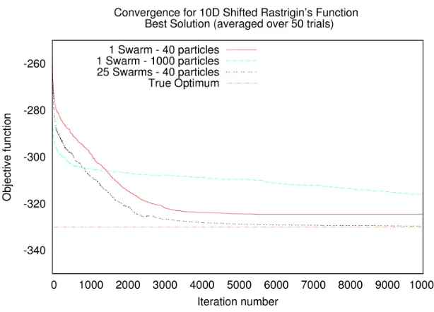
6.3 Rastrigin function: Extended analysis . . . 69
6.3.1 Impact of Swarm Size . . . 69
6.3.2 Multi-Swarm Performance . . . 70
6.4 CEC 2012 results . . . 73
6.5 WDS: Standard PSO Performance . . . 81
6.5.1 Complex Search Problems . . . 82
6.6 Observations . . . 85
Chapter 7 TAPSO: Topology Aware Particle Swarm Optimization . . . 86
7.1 Motivation . . . 86
7.2 Design . . . 87
7.3 Results . . . 92
7.3.1 Visualization . . . 93
7.3.2 Multi-Leak Scenario: Preliminary Studies . . . 96
Chapter 8 Optimus Performance Model . . . 99
8.1 Performance Model Parameters . . . 99
8.2 Computation Time . . . 101
8.3 Communication Time . . . 101
8.4 Model Validation . . . 105
Chapter 9 Conclusions and Future Work . . . 106
9.1 Conclusions . . . 106
References . . . 109
Appendix . . . 115
Appendix A ASCEM-IO: Parallel I/O library . . . 116
A.1 Introduction . . . 117
A.2 PFLOTRAN . . . 118
A.2.1 PFLOTRAN I/O . . . 119
A.2.2 Performance . . . 120
A.3 Optimized I/O pattern . . . 121
A.4 ASCEM-IO library . . . 125
A.4.1 Related Work . . . 126
A.4.2 Architecture . . . 126
A.4.3 Supported I/O Patterns . . . 128
A.4.4 Brief description of user callable routines . . . 129
A.5 Performance . . . 130
A.6 Future Work . . . 134
LIST OF TABLES
Table 4.1 WDS Problems: Weighting factors . . . 35
Table 6.1 Standard PSO: Algorithmic Parameters used in this analysis . . . 54 Table 7.1 TAPSO: Algorithmic Parameters used in this analysis . . . 92
LIST OF FIGURES
Figure 3.1 Architecture of the Optimus framework . . . 21
Figure 3.2 Cooperative Multi-Swarm Optimization Framework with algo-rithm to system architecture mapping . . . 22
Figure 3.3 Optimus Communication patterns: (a) Optimizer-Evaluator in-teractions each iteration and (b) Inter-Optimizer communication performed every few iterations (configurable algorithmic param-eter) . . . 28
Figure 4.1 Architecture of Cray XT5 (JaguarPF) . . . 37
Figure 4.2 Architecture of IBM BlueGene/P (Intrepid) . . . 38
Figure 4.3 Profiling results of a serial EPANET execution: list of functions in descending order of exclusive time taken . . . 39
Figure 4.4 Scalability bottleneck of baseline EPANET using temporary hy-draulics files . . . 39
Figure 4.5 Water Distribution System network (Network2) used for parallel CRS study . . . 41
Figure 4.6 Improved EPANET: Using in-memory buffer instead of tempo-rary hydraulics files . . . 42
Figure 5.1 Micropolis: A medium-sized water distribution network used in weak scaling experiments . . . 44
Figure 5.2 Optimus: Weak Scaling Performance - X-axis represents the num-ber of cores and numnum-ber of swarms in each case are indicated in parenthesis. . . 45
Figure 5.3 Weak Scaling: Number of simulations per minute . . . 46
Figure 5.4 Weak Scaling: Number of simulations per minute per core . . . . 47
Figure 5.5 Extended weak scaling results from 1 to 200,000 cores . . . 48
Figure 5.6 Performance Impact of Number of Swarms . . . 49
Figure 5.7 Performance Impact of Swarm Size . . . 50
Figure 6.1 Surface plot of 2D Shifted Sphere function . . . 56
Figure 6.2 Surface plot of 2D Shifted Rosenbrock function . . . 56
Figure 6.3 Surface plot of 2D Shifted Rastrigin function . . . 57
Figure 6.4 Surface plot of 2D Schwefel’s function . . . 57
Figure 6.5 Surface plot of 2D Shifted Schwefel’s function . . . 58
Figure 6.6 Surface plot of 2D Shifted Rotated Griewank’s function . . . 58
Figure 6.9 Shifted Rosenbrock’s function: Convergence pattern of a typical swarm . . . 60 Figure 6.10 Shifted Rastrigin’s function: Convergence pattern of a typical
swarm . . . 61 Figure 6.11 Shifted Rastrigin’s function: Convergence pattern of a larger
swarm compared to baseline swarm . . . 62 Figure 6.12 Shifted Rastrigin’s function: Convergence pattern using four
cooperative swarms . . . 62 Figure 6.13 Shifted Schwefel’s function: Convergence pattern of a typical
swarm . . . 63 Figure 6.14 Shifted Griewank function: Convergence pattern of a typical swarm 64 Figure 6.15 Shifted Griewank function: Convergence pattern using four
co-operative swarms . . . 64 Figure 6.16 Shifted Ackley’s function: Convergence pattern of a typical swarm 65 Figure 6.17 Shifted Sphere function: Convergence of a single swarm - X-axis
shows the iteration number and Y-axis shows the average of best solution for each iteration from 50 trials . . . 66 Figure 6.18 Shifted Rosenbrock’s function: Convergence of a single swarm
-X-axis shows the iteration number and Y-axis shows the average of best solution for each iteration from 50 trials . . . 66 Figure 6.19 Shifted Rastrigin’s function: Convergence of a single swarm-
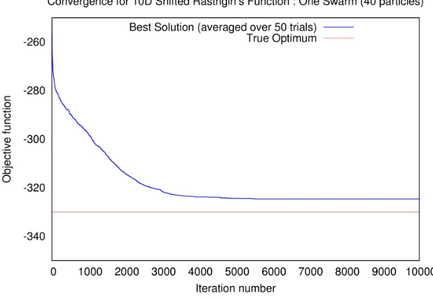
X-axis shows the iteration number and Y-X-axis shows the average of best solution for each iteration from 50 trials . . . 67 Figure 6.20 Shifted Schwefel’s function: Convergence of a single swarm
-X-axis shows the iteration number and Y-axis shows the average of best solution for each iteration from 50 trials . . . 67 Figure 6.21 Shifted Griewank function: Convergence of a single swarm -
X-axis shows the iteration number and Y-X-axis shows the average of best solution for each iteration from 50 trials . . . 68 Figure 6.22 Shifted Ackley’s function: Convergence of a single swarm -
X-axis shows the iteration number and Y-X-axis shows the average of best solution for each iteration from 50 trials . . . 69 Figure 6.23 Convergence of a single swarm using function - X-axis shows the
iteration number and Y-axis shows the average of best solution for each iteration from 50 trials . . . 70 Figure 6.24 Shifted Rastrigin’s function: Comparison of swarm size vs.
Figure 6.25 Shifted Rastrigin’s function: Impact of multiple swarms on con-vergence - X-axis shows the iteration number and Y-axis shows the average of best solution for each iteration from 50 trials . . . 72 Figure 6.26 Shifted Griewank function: Convergence of a single swarm -
X-axis shows the iteration number and Y-X-axis shows the average of best solution for each iteration from 50 trials . . . 72 Figure 6.27 1000D Ackley’s function: Convergence using 32 swarms -
X-axis shows the iteration number and Y-X-axis shows the objective function value of best solution for each iteration averaged across 10 trials. . . 73 Figure 6.28 1000D Elliptic function: Convergence using 32 swarms - X-axis
shows the iteration number and Y-axis shows the objective func-tion value of best solufunc-tion for each iterafunc-tion averaged across 10 trials. . . 74 Figure 6.29 1000D Elliptic function: Convergence using 32 swarms - X-axis
shows the iteration number and Y-axis (log scale) shows the ob-jective function value of best solution for each iteration averaged across 10 trials. . . 75 Figure 6.30 1000D Rastrigin’s function: Convergence using 1, 32 and 64
swarms - X-axis shows the iteration number and Y-axis shows the objective function value of best solution for each iteration averaged across 10 trials. . . 75 Figure 6.31 1000D Rastrigin’s function: Convergence comparison with
dif-ferent number of swarms - X-axis shows the iteration number and Y-axis shows the objective function value of best solution for each iteration averaged across 10 trials. . . 76 Figure 6.32 1000D Rastrigin’s function: Convergence using 32 swarms with
different population sizes - X-axis shows the iteration number and Y-axis shows the objective function value of best solution for each iteration averaged across 10 trials. . . 77 Figure 6.33 1000D Shifted Rastrigin’s function: Convergence using 64 swarms
- X-axis shows the iteration number and Y-axis shows the objec-tive function value of best solution for each iteration averaged across 10 trials, the error bars indicate standard deviation among the trials. . . 78 Figure 6.34 1000D Rosenbrock’s function: Convergence using 32 swarms
Figure 6.35 1000D Rosenbrock’s function: Convergence using 32 and 64 swarms - X-axis shows the iteration number and Y-axis shows the objective function value of best solution for each iteration averaged across 10 trials. . . 79 Figure 6.36 1000D Rosenbrock’s function: Convergence using 32 and 64
swarms - X-axis shows the iteration number and Y-axis (log scale) shows the objective function value of best solution for each iteration averaged across 10 trials. . . 79 Figure 6.37 1000D Schwefel’s function: Convergence using 32 swarms -
X-axis shows the iteration number and Y-X-axis shows the objective function value of best solution for each iteration averaged across 10 trials. . . 80 Figure 6.38 1000D Schwefel’s function: Convergence using 32 swarms -
X-axis shows the iteration number and Y-X-axis (log scale) shows the objective function value of best solution for each iteration averaged across 10 trials. . . 81 Figure 6.39 Network2: A large water distribution system used to study
con-vergence. Cyan-colored nodes represent sensor locations, red-node denotes true leak location and green-colored red-node repre-sents best estimate found by the optimization method. . . 82 Figure 6.40 Single leak scenario convergence . . . 83 Figure 6.41 Ten leaks scenario convergence: Impact of swarm size . . . 84 Figure 6.42 Ten leaks scenario convergence: One and Two Swarms comparison 85 Figure 7.1 Standard PSO: Potential locations after position update. . . 87 Figure 7.2 TAPSO: Distance to Global and Personal Bests influence new
position of particle. . . 88 Figure 7.3 TAPSO: Distance to Global and Personal Bests have competing
influence on new position of particle. . . 89 Figure 7.4 Standard PSO vs. TAPSO: Convergence comparison - Best
solu-tion averaged across 25 trials . . . 92 Figure 7.5 TAPSO: Convergence - Box plot comparing standard PSO and
TAPSO . . . 93 Figure 7.6 TAPSO: Visualization results from a trial - Iteration 1 (beginning) 94 Figure 7.7 TAPSO: Visualization results from a trial - Iteration 14
(interme-diate) . . . 95 Figure 7.8 TAPSO: Visualization results from a trial - Iteration 50 (end) . . . 96 Figure 7.9 Network2 - 4-leak scenario: Convergence using TAPSO (10 swarms) 97 Figure 7.10 Network2 - 4-leak scenario: Solution found using TAPSO (10
Figure 8.1 Optimus Weak Scaling Study: Comparison of predicted val-ues from performance model to actual performance results on
JaguarPF (Cray XK6) supercomputer. . . 105
Figure A.1 PFLOTRAN Default I/O access patterns . . . 119
Figure A.2 PFLOTRAN performance on Jaguar using default I/O . . . 121
Figure A.3 Optimized two-phase I/O access patterns . . . 122
Figure A.4 Performance of optimized PFLOTRAN Initialization phase on Jaguar . . . 124
Figure A.5 Performance of optimized PFLOTRAN write phase on Jaguar . . 125
Figure A.6 Overall architecture of the ASCEM-IO library . . . 127
Figure A.7 Supported Access Patterns . . . 128
Figure A.8 I/O performance of default I/O (HDF collective) with two-phase ASCEM-IO library. At 144k cores the wallclock time for default I/O method is 535 secs compared to 129 secs for two-phase library method for the 14 GB file scenario. . . . 132
Figure A.9 Detailed performance analysis of Parallel I/O benchmark. . . 132
LIST OF ALGORITHMS
CHAPTER 1
Introduction
This research describes the design and development of a parallel optimization frame-work for scientific applications. Specific problems investigated in this frame-work include optimization problems in Water Distribution Systems. This chapter provides an intro-duction to optimization problems and algorithms. It introduces relevant terminology that lay the groundwork for subsequent chapters.
1.1
Optimization Problems
the problem has one objective or (b) Multi-objective: if the problem has more than one objective. Specifically, the class of multi-objective problems are challenging because the relationships among the multiple objectives (cooperative or competitive) may not be knowna priorifor a given problem.
Additionally, optimization problems can be (a) constrained: if some constraints are defined for parameters to be acceptable towards a solution or (b) unconstrained: if no such constraints exist. Moreover, optimization problems can be classified as (a) linear optimization (linear programming): if the objective function and constraints are derived from linear relationships among the parameters, or (b) non-linear opti-mization: if the objective function or any existing constraint is composed of non-linear relationships among the parameters.
An optimization problem is feasible if at least one solution exists that can satisfy the constraints and maximize/minimize the objective function as specified. If no such solution exists, then the problem is infeasible. An optimization problem is said to be multi-modal if there are multiple locally optimal solutions to the specified objective(s).
In the case of linear programming, existing algorithms such as the simplex method can formally guarantee convergence if a feasible solution exists. Algebraic Modeling languages such as AMPL, GAMS or Mathprog are typically used to model linear programming problems. Such problems are then handed over to solvers provided by open-source tools like GLPK (GNU Linear Programming Toolkit) [1] or commercial solvers like CPLEX[2]. A notable recent entry is Python Optimization Modeling Objects (Pyomo)[3], an open source tool for modeling optimization applications that provides the benefits of an algebraic modeling language while providing the flexibility of working within a fully functional programming language environment.
guar-antee convergence for an arbitrary nonlinear optimization problem. If the objective function is well-defined, continuous and differentiable, then techniques like gradient based algorithms can be used to find the optimal solution. Still, such techniques may become trapped in a local optimum if the objective function has multiple local-optima (multiple points in the search space where gradient is zero).
On the other hand, numerous scientific and engineering optimization problems have complex and sometimes ill-understood relationships between parameters and objectives. Moreover, some problems are essentially treated as black-box models wherein non-linear effects of parameters on objectives are observed but the specific dynamics of such interactions is unknown. Traditional mathematical optimization algorithms prove ineffective and there might be no known polynomial-time algorithms for tackling such problems.
Heuristic optimization methods are typically used in such scenarios (black-box) as they make few or no assumptions about the problems being solved. They attempt to solve an optimization problem by iteratively improving a candidate solution(s) with respect to a given quantitative metric. A population based heuristic method is one that maintains and iterates over a pool of candidate solutions during the search process. They usually incorporate a form of stochastic optimization, wherein random numbers are generated and used to guide the decision process during iteration. A comprehensive introduction to widely used heuristics including genetic algorithms, swarm optimization, simulated annealing etc. is provided by Engelbrecht [4]. A heuristic algorithm cannot formally guarantee optimality and its efficacy is often demonstrated empirically for a specific problem.
possible problems is identical. This also holds true for stochastic ‘non-potentially revisiting’ algorithms. However, in practice one typically encounters a smaller subset of optimization problems that exhibit similar characteristics. This theorem demon-strates that whatever gains an algorithm obtains on one class of problems is offset by its degradation on remaining problems. Thus, we cannot accurately compare two algorithms based on their performance on a small sample of problems. These theorems also reinforce the importance of incorporating problem-specific knowledge into the algorithm to be effective at solving a particular class of problems. So, a practitioner can develop a customized heuristic optimizer that can perform well empirically on problems of interest. Bearing that in mind, one can strive to tune heuristic methods to achieve a desired convergence performance for a target application.
1.2
Primer on Evolutionary Algorithms
Evolutionary algorithms (EA) are perhaps the most widely used heuristic optimization methods. They are inspired by biological evolution wherein candidate solutions are evolved in a process akin to natural evolution. In EA terminology, a candidate solution is termed as an individual and the set of such solutions is known as a population. During each iteration (generation in EA parlance), individuals are mixed using se-lection, recombination/crossover and mutation operations to derive the individuals of the next generation. The individuals with better fitness are usually selected to be combined to produce the next generation. Algorithm 1.1 illustrates the steps involved in a standard evolutionary algorithm.
in-dividuals are randomly chosen and the individual with the best fitness is selected. During recombination operation, parameters of two selected individuals are combined to produce offspring’s parameter set. If the parameters are binary encoded, recom-bination operations such as single-point or multi-point crossover is generally used. In the case of continuous optimization problems, simulated binary crossover (SBX) [6] is typically employed. During mutation operation, parameters of an individual are perturbed usually using a Gaussian distribution to generate parameters for an individual for the next generation. Please refer to Mitchell [7] for further details on evolutionary operators. This process of selection, crossover and mutation is repeated until termination criteria is met.
Algorithm 1.1Outline for Canonical Evolutionary Algorithm. 1: GenerateInitialPopulation(pop)
2: for individual←1 topopSizedo
3: Evaluate(individual)// Compute Objective function value 4: end for
5: while !StopCondition()do 6: parents ←Selection(pop)
7: forindividualssubject to recombinationRate do 8: offspring←Recombination(parents)
9: end for
10: forindividualssubject to mutationRatedo 11: offspring←Mutation(offspring); 12: end for
13: forindividual ←1topopSizedo
14: Evaluate(individual) // Compute Objective function value 15: end for
16: end while
Strength Pareto Evolutionary Algorithm (SPEA)[9] are two prominent techniques used in the field. Coello et al. [10] provides a detailed survey of multi-objective evolutionary approaches. The reader is referred to Deb [11] for further exploration of evolutionary MOO.
1.3
Primer on Swarm Optimization algorithms
Particle swarm optimization (PSO) is a swarm intelligence method wherein particles (candidate solutions) are ‘flown’ across parametric space to find optimal values [12; 13]. It is a global optimization technique that belongs to the class of direct search methods. This method emulates the flocking or swarming behavior observed in nature among groups of birds or fish [14]. Each candidate solution is represented as a particle in the
n-dimensional problem space and has an associated position and velocity attributes where n is the number of parameters being optimized. During every iteration, the velocity and position of a particle are updated using the information gleaned from that iteration to guide the search process. Each particle’s position is influenced by the best position it has found so far (cognitive component) as well as the best position found by other particles in the swarm (social component). This method strives to find the optimal solution by learning and sharing such information among particles in the problem space.
Algorithm 1.2Outline for Particle Swarm Optimization. 1: GenerateInitialPopulation(pop)
2: for particle←1tonumParticles do
3: Evaluate(particle)// Compute Objective function value 4: end for
5: while !StopCondition()do 6: GetGlobalBest(pop)
7: forparticle←1 tonumParticlesdo
8: neighbors←CalculateNeighborhood(topology,Position(particle)) 9: optionalGetNeighborhoodBest(neighbors)
10: UpdateVelocity(particle) 11: UpdatePosition(particle) 12: end for
13: forparticle←1 tonumParticlesdo
14: Evaluate(particle)// Compute Objective function value 15: end for
16: end while
−→vt
i =wt−→vt
−1
i +c1ψ1(
−→p
i−
−→
Xti−1) +c2ψ2(−→pnb−
−→
Xit−1) (1.1a)
−→
Xit =−→Xit−1+∆−→Xti
| {z }
χ−→vit
(1.1b)
−→
Xti and−→vti represent the position and velocity vectors respectively of particlei dur-ing iterationt. Equation 1.1a illustrates the UpdateVelocityoperation that is performed every iteration. −→pi denotes the personal best position found so far by a particle and
−→p
of a particle to continue with its previous velocity (inertia). It limits the rate at which particles agglomerate in problem space promoting better exploration. Larger values ofwt facilitate global exploration at the expense of convergence time, while smaller values of wt result in shorter convergence time, but could result in convergence to a local optimum.wt is either kept constant throughout the experiment or gradually reduced over iterations to reduce the search space that a particle explores. Clerc [13] proposed another parameter χ, constriction coefficient (similar to inertial coefficient) to prevent particle explosion (scattering) in problem space.
c1 represents the cognitive coefficient that influences the pace at which a particle learns from its own experience so far. c2 denotes the social efficient that determines how quickly information from other particles are incorporated in a particle’s velocity. The cognitive and social coefficients drive towards exploitation of the search space. Care must be taken to balance the exploratory and exploitative algorithms to avoid premature convergence. The case ofc1 >c2facilitates global exploration at the expense of convergence time, while the case of c2 > c1 reduces the convergence time at the expense of robustness. The reader is referred to van den Bergh [15] for guidance on choosing appropriate values of PSO parameters. Typical values used in literature [4] include c1,c2 ∈[0.5, 2.5],w ∈ [0, 1)and χ∈ [0, 1].
Consider the scenario where all particles constitute a single neighborhood, the cognitive component includes the global best position −→pg and such variant of the swarm optimizer is known as gbest PSO. In contrast, when fewer particles form localized neighborhoods and share local best−→pl information, it is known as albest
PSO. Ahybrid PSO is a variant that combines aspects of bothgbest andlbestupdate schemes.
Vmax to prevent scattering of the particles. Clerc and Kennedy [16] led a thorough investigation into the effects of parameters on a particle’s movement and proposed a bounded variant of the algorithm to prevent explosion(scattering) of particles without usingVmax.
Kennedy [17] explored the effects of neighborhood topology on the efficacy of the search process. Suganthan [18] suggested using dynamic neighborhood topology to improve PSO performance. Akat and Gazi [19] compare three neighborhood strategies and presented performance results for several analytical test problems (Rastrigin, Griewank etc.). The topologies studied include nearest neighbors in problem space, objective space and random neighbors.
For multi-objective problems, Hu and Eberhart [20] proposed a PSO method that obtains a pareto-optimal set of solutions instead of a single solution. The major modifications that were done to standard PSO to adapt to multi-objective problems are (a) a dynamic neighborhood strategy based on fitness values, (b) personal best (pBest) update using only those solutions that dominate currentpBestand (c) one-dimension optimization: optimizing one objective at a time.
Algorithm 1.3 illustrates the outline for a cooperative multi-swarm method. In addition to the standard PSO operations, there is an additional migration phase in the multi-swarm approach.
Algorithm 1.3Outline for Cooperative Multiple Swarms. 1: GenerateInitialPopulation(pop)
2: for particle←1tonumParticles do
3: Evaluate(particle)// Compute Objective function value 4: end for
5: while !StopCondition()do 6: GetGlobalBest(pop)
7: forparticle←1 tonumParticlesdo
8: neighbors←CalculateNeighborhood(topology,Position(particle)) 9: optionalGetNeighborhoodBest(neighbors)
10: UpdateVelocity(particle) 11: UpdatePosition(particle) 12: end for
13: forparticle←1 tonumParticlesdo
14: Evaluate(particle)// Compute Objective function value 15: end for
16: iftime for migration then
17: // every m iterations where m is migration frequency
18: SendMigrantsToNeighboringSwarm() 19: RecvMigrantsFromNeighboringSwarm()
20: // Integrate incoming migrants into swarm
21: end if 22: end while
1.4
Organization
The rest of the dissertation is organized as follows. Chapter 2 provides a summary of existing parallel optimization techniques. Section 2.2 describes approaches in parallel particle swarm methods. Parallel evolutionary algorithms are summarized in section 2.3.
Chapter 3 describes the design and development of Optimus, a parallel optimiza-tion framework. Chapter 4 introduces two optimizaoptimiza-tion problems pertaining to Water Distribution Systems (WDS).
We describe computational performance results using Optimus for WDS applica-tions on a Cray XK6 supercomputer in Chapter 5. We discuss algorithmic performance of PSO for benchmark test problems and WDS applications in Chapter 6.
Chapter 7 describes a new optimization technique, TAPSO (Topology Aware Particle Swarm Optimization) that is targeted towards problems with an underlying graph structure in the search space.
CHAPTER 2
Parallel Metaheuristics
This chapter provides a summary of existing parallel optimization techniques. Section 2.2 describes approaches in parallel particle swarm methods. Parallel evolutionary algorithms are summarized in section 2.3.
Metaheuristics are a class of algorithms that try to find an best-effort solution for an optimization problem but they would not guarantee convergence. The reader is referred to Talbi et al. [21] for alternate approaches in parallel metaheuristics.
2.1
Metrics
This section introduces several metrics to measure the performance of an optimization method. This includes algorithmic measures such as number of iterations to converge as well as computational performance metrics such as speedup and parallel efficiency. These metrics provide required guidance while comparing different optimization techniques.
2.1.1
Algorithmic Performance Metrics
A specific optimization technique can be measured by the number of objective function evaluations computed for obtaining the optimal solution. For an iterative method, it can also be measured by the number of iterations or generations to obtain a solution within a desired threshold. In cases where the practitioner is unaware of the objective space, different methods can be compared by the best solution found by each method within a specified duration.
several optimizers.
If a mix of serial and parallel optimizers are being compared, number of evaluations can be used as a first metric. It must be noted that it may not capture the implications of differences between serial and parallel algorithms. For further discussion, please refer to Alba and Tomassini [22].
2.1.2
Parallel Performance Metrics
Speedup (S) is a metric used to characterize the parallel performance of an application. It is calculated using equation 2.1a. It is the ratio of the serial runtime of the sequential algorithm for solving a problem (Tserial) to the time taken by a parallel algorithm (Tparallel) to solve the same problem onpprocessing elements (PEs). It is assumed that the serial and parallel algorithms use an identical processing element; the parallel variant using pprocessing elements in this scenario.
Parallel efficiency is a related performance metric to measure the fraction of time a processing element is usefully employed. Equation 2.1b illustrates that efficiency is the ratio of the speedup of a given parallel algorithm to the number of processing elements. In the ideal scenario, speedup is equal top resulting in an efficiency of 1. However, in practice speedup is less thanpdue to communication and other system overheads. So efficiency is typically between zero and one depending on the efficacy of the parallel algorithm to utilize the processing elements.
speedup S= Tserial Tparallel
(2.1a)
efficiency E= S
Furthermore, there are two basic scenarios for measuring the scalability of an application.
1. In the strong scaling scenario, the problem size is kept fixed as the number of processing elements is increased. The strong scaling efficiency (as a percentage of baseline) is shown in Eq. 2.2a where Tbaselinerepresents the time to completion in the baseline case (typically using a single processing element) and TSlargePE represents time to completion for the same problem using a larger number of processing elements (in this case p).
2. In theweak scalingscenario, the problem size (workload) is increased correspond-ing with an increase in the number of processcorrespond-ing elements employed. The intent is to keep the amount of work performed by each PE fixed as the number of PEs is increased. Eq. 2.2b computes the weak scaling efficiency as a percentage of baseline performance (Tbaseline and TWlargePE denotes the time to completion for the larger problem using a higher number of PEs.
Strong Scaling Estrong =
p∗TSlargePE
Tbaseline
∗100 (2.2a)
Weak Scaling Eweak =
Tbaseline
TWlargePE
∗100 (2.2b)
2.2
Parallel Swarm algorithms
In case of parallel PSO algorithms, initial efforts were focused on parallelizing objec-tive function evaluations. Schutte et al. [24] proposed a parallel global optimization method using PSO and presented results for analytical test problems as well as for a biomechanics problem. They observed that parallel efficiency decreased almost linearly with increasing number of processing elements(PEs) for the biomechanics test problem which exhibited load imbalance. They also identified synchronization require-ment at each iteration to be a bottleneck and suggested investigation of asynchronous implementations.
Koh et al. [25] developed PAPSO, a parallel asynchronous PSO algorithm where the particles are permitted to change continuously instead of every iteration. This entails performing updates to a particle’s velocity and position whenever new results are available thereby eliminating per-iteration updates to velocity and position. They have demonstrated improvement obtained over synchronous PSO for analytical test problems up to 32 processors. Recently Li [26] introduced a similar scheme called delayed exchange parallel PSO wherein the best fitness exchanged are staggered for a configurable number of iterations. The speedup results presented for analytical problems on 16 processors ranged from 13.2 (Rosenbrock function) to 15.2 (Ackley function).
2.2.1
Limitations
parallelization scheme. Even for analytical test problems that usually exhibit no imbalances across multiple evaluations, these frameworks have not achieved ideal parallel speedups.
Furthermore, the asynchronous designs of earlier studies [25; 26] were focused on avoiding the synchronization required at each iteration. They have not explored multi-swarm designs in parallel. Some existing designs also incorporate an implicit assumption that the objective function evaluation is computationally much more expensive than any requisite computation performed within the framework.
2.3
Parallel Evolutionary algorithms
Alba et al. [22] classify existing parallel evolutionary algorithms as follows:
• Panmictic Master-worker GAs: In this scenario, parallelization is performed across independent objective function evaluations. Panmictic population refers to the characteristic where individuals can potentially mate with any other individual in the population.
• Island model GAs: In this case, there is one master and its associated workers per island. The master processes of different islands communicate periodically to exchange information and facilitate migration of best individuals. Unlike panmictic populations, global population is divided into sub-populations that are structured within islands, thereby limiting individuals to mix with others within the island. This is a coarse-grained distribution scheme where each sub-population consists of a large number of individuals.
population is divided into sub-populations that typically contain just a single individual.
There are some hybrid schemes that display attributes of both island and cellular GAs. Cantú-Paz [27] provides a thorough introduction and empirical guidance to the design of efficient parallel genetic algorithms. This work also presents some insight into migration rates and optimal communication topologies.
For parallel multi-objective optimization, Durillo et al. [28] presented a master-worker as well as asynchronous parallelization scheme for NSGA-II.
2.4
Optimization frameworks
2.5
New Contributions
• While existing parallel optimization frameworks [29; 35; 34; 30] are useful in their own way and can be applied to a wide class of problems, the asynchronous design choices in our framework enable us to scale to hundreds of thousands of cores.
• There is a body of work that captures multi-island dynamics [27] (for genetic algorithms) but an equivalent investigation of multi-swarm behavior does not exist. Due to the inherent differences in sharing of information between evo-lutionary and particle swarm optimization methods, further investigation is warranted to understand multi-swarm interactions. This work lays the founda-tion to investigate several interacfounda-tion patterns and develop insights for designing better multi-swarm algorithms.
• Wolpert and Macready [5] emphasize the importance of incorporating problem-specific knowledge into the algorithm to be effective at solving a particular class of problems. This research involves design of customized optimization techniques (TAPSO: See Chapter 7) for target scientific applications.
CHAPTER 3
Optimus Optimization Framework
This chapter describes the design and development of Optimus, a parallel optimization framework. We describe computational performance results using Optimus for WDS applications on a Cray XK6 supercomputer in Chapter 5. We discuss algorithmic performance in Chapter 6.
3.1
Optimus
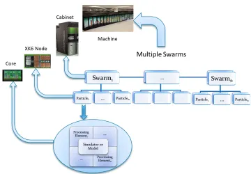
experimen-Figure 3.1: Architecture of the Optimus framework
tation with communication and migration patterns among the optimizers. Optimus currently includes a parallel search algorithm, COMSO (Cooperative Multi-Swarm Optimization) based on Particle Swarm Optimization (PSO) for addressing generic optimization problems.
Figure 3.2: Cooperative Multi-Swarm Optimization Framework with algorithm to system architecture mapping
multi-level parallelism as illustrated here in the case of Cray XK6. Hence this kind of algorithm-system mapping would be feasible on other supercomputing architec-tures too. This would also enable the framework to adapt to emerging many-core heterogeneous supercomputing architectures that include accelerators such as GPUs.
Optimus consists of the following major components as shown in Figure 3.1:
• Evaluator Module: This provides a streamlined interface to the optimization problem. The functions within this module are invoked by the driver program to compute the objective function value of the target application with given set of parameters.
• PRIME:ParallelReconfigurableIterativeMiddlewareEngine provides capabili-ties for parameter distribution, results aggregation and inter-optimizer commu-nication. See section 3.3 for details.
• Utilities: Output module provides parallel I/O functionality to record simulation and optimizer results during the search process. Visualization module processes the output to track and plot search progress. An extensible module for parallel random number generators was developed.
• Driver Module: The driver module integrates the rest of the components to-gether, handles the control-flow to drive program execution.
The rest of this section elaborates on key components while PRIME is described in Section 3.3.
3.1.1
Evaluator Module
3.1.2
Optimizer Module
This is an interface provided to an arbitrary population-based optimization algorithm. It provides function entry points to perform algorithm initialization, generate a set of evaluations, import results for a set of evaluations and termination at the end. This module interacts with the parallel middleware to distribute the objective function evaluations (i.e., simulations) and retrieve the results upon completion. Subsequently, post-processing tasks specific to the optimization method are executed to generate the population of candidate solutions for the next iteration.
The optimizer is also responsible to signal completion (i.e., when a set number of iterations are completed or when the objective function value reaches the de-sired threshold). Presently, Optimus can interface with optimizers written in C, C++. Optimus itself is written in C.
Swarm optimizer
As part of this research, we developed a multi-swarm optimizer that implements a standard PSO algorithm [39] includinggbest,lbestandhybridvariants (see Chapter 1.3). Furthermore, we incorporated a new PSO technique, TAPSO (see Chapter 7) for network-based problems in this optimizer.
3.2
Utilities
3.2.1
Output Module
In order to handle the large quantity of data produced by Optimus, we utilized a scalable application layer parallel I/O library [40] that we developed earlier. Each opti-mizer creates a HDF5 (Hierarchical Data Format) file to store parameters, results and other algorithm-specific attributes periodically. Such files are subsequently used for generating reports during post-processing and visualization. Additional information on the parallel I/O library is presented in Appendix A.
3.2.2
Visualization Module
This module processes Optimus output files and generates lucid visualizations de-picting search progress. It includes plotting and animation capabilities for visualizing candidate solutions in parametric space during the search process. The visualization tool is built using Python and utilizes Matplotlib [41] and h5py [42] libraries. It is generic and can be coupled with any optimizer in the Optimus framework easily.
Furthermore, we have designed another visualization tool specifically for Water Distribution Systems applications. It can overlay the search results from the optimiza-tion algorithm, e.g., best leak locaoptimiza-tion found on top of the specific water network used in the experiment. E.g., see Figure 7.6 and related discussion in Chapter 7.
3.2.3
Configuration File Parser
and broadcast to the rest. The former option is a potential performance bottleneck as it induces stress on the file system when a large number of processes are accessing the same file. Alternately, the latter option could be cumbersome to maintain since the broadcast subroutine has to be updated whenever additional details are added to configuration file.
Hence, a configuration file parser was developed to facilitate the second usage pattern wherein the required configuration file is read into a buffer and broadcast to all processes. A simplified API is provided to parse a configuration file in an arbitrary text (ASCII) format or YAML [43], a human friendly data serialization format. It supports parallel file-read-broadcast pattern to reduce I/O contention. The parsing logic can then be reused by all processes.
3.2.4
Random Number Generator
Heuristic optimization algorithms are stochastic techniques that utilize random vari-ables during the search process. Hence the quality of random numbers is crucial for these methods. An extensible wrapper for random number generators was developed to encapsulate specialized parallel random number generator libraries like SPRNG [44] in addition to ubiquitous Linuxrand(used as a fallback option). This provides the flexibility of choosing the best variant available on a specific computational platform.
3.2.5
Statistics Module
A statistics module was developed to help study the efficacy and progress of the search process. This includes computation of mean and standard deviation of objective values, centroids of candidate solutions in parametric and objective space.
3.3
PRIME
PRIME refers to Parallel Reconfigurable Iterative Middleware Engine. It utilizes the Message Passing Interface(MPI) [48] for parallelism. PRIME implements the decen-tralized manager-worker paradigm for parallel execution. In its basic configuration, there would be one manager process and several associated workers. For complex scenarios like multi-swarms, there would be several manager processes and their corresponding workers. The manager processes execute the optimizer component and the workers would execute the simulator/evaluator component for the target application. PRIME provides a well-defined interface for different optimizers to share search information among themselves efficiently. Additionally, it utilizes asynchronous communication primitives to enable overlapping communication with computation within the optimizer.
3.3.1
Communication Patterns
Figure 3.3: Optimus Communication patterns: (a) Optimizer-Evaluator interactions each iteration and (b) Inter-Optimizer communication performed every few iterations (configurable algorithmic parameter)
Figure 3.3 shows the communication patterns in PRIME. The first pattern describes the optimizer-evaluator interactions where the evaluator receives set of parameters, computes the simulations and then return the results back to the optimizer. The second pattern shows the inter-optimizer data exchange protocol.
best solution to the next swarm periodically, specifically every five iterations for the weak scaling scenario presented.
Static/Dynamic load balancing
PRIME enables both static and dynamic load balancing schemes for distributing simulations among the available evaluators.
Static load balancing results in equal partitioning of required simulations in an iteration. However, in dynamic load balancing, all evaluators initially get one set of simulations and the next set is sent in the order of completion. Additionally, PRIME supports chunking/pooling of simulations. The pool size is a configurable parameter that can be adjusted as required.
If the evaluator exhibits little or no variability in computing different candidate solutions (simulations), then static load balancing is preferred as it results in fewer messages. Otherwise, if there is significant variability among different simulations, then dynamic load balancing scheme with a suitable pool size should be used. The pool size depends on the degree of variability in evaluations of a specific problem on a computational platform. Hence, the pool size is a user-defined parameter that is usually chosen empirically.
3.3.2
Optimizer Communicators and Topologies
In the case of multiple swarms, we utilize the communicator functionality of MPI to create a logical grouping of processes for each swarm. The global MPI communicator is divided into multiple sub-communicators (one per swarm) using the MPI_Comm_-split()operation. An additional communicator exclusively for optimizers is created to simplify data sharing. Swarms can communicate within the group using the intra-optimizer communicator and exchange information with other swarms using inter-optimizer communicator. The inter-optimizer communicator could reflect a sim-ple topology like ring or emulate a custom problem-dependent structure. In order to facilitate lightweight communication among optimizers, non-blocking communi-cation primitives (e.g.,MPI_Isend, MPI_Irecv) are used to overlap computation and communication.
CHAPTER 4
Preliminary Studies: Water Distribution
Systems Applications
This chapter introduces the contaminant source characterization and leak detection problems in water distribution systems and elaborates upon the problem formulation. We also provide detailed performance analysis of the simulator, identify performance bottlenecks and describe enhancements implemented to improve computational per-formance of the simulator.
4.1
Motivation
intentional contamination incidents that could result in adverse human health and safety impacts. Identifying contamination events is therefore of high priority for municipal authorities to rapidly deploy mitigation actions. Usually, a water network is highly interconnected intentionally to facilitate redundant flow paths, and experiences significant and frequent fluctuations in flows and transport paths. These network characteristics inadvertently enable contamination in one part of the network to spread rapidly via different pathways through the network, unbeknownst to consumers. When a contamination event is detected via the first line of defense, e.g., data from a water quality surveillance sensor network and reports from consumers, the municipal authorities need to rapidly predict the source characteristics (such as location, and time of release and mass loading history), estimate the extent of the contamination in the network through simulation and confirmatory sampling, and prescribe control actions (such as flow controls using valves, hydrants and storage units, or injection of decontaminants) to mitigate the event.
A typical WDS contains miles of buried pipes and thousands of fixtures, where every component is susceptible to physical damage due to old age, corrosion and deterioration over time. Such leaks can lead to the significant loss of water during distribution before reaching the customers. Water customers are metered for usage at end point only, hence any loss of water due to leaks is attributed as Non Revenue Water (NRW). Hence, leaks due to breakage of pipes can be potential intrusion points for contamination as well as lead to significant economic losses for the utilities.
framework [49].
The aforementioned issues, contaminant source characterization and leak detection are difficult combinatorial optimization problems with a mixture of discrete and continuous variables. While solving such problems for a large WDS is difficult, trying to identify multiple leaks or contaminant source locations is much harder due to combinatorial explosion.
4.2
Water Distribution Systems Simulator
Our simulation component is based on EPANET [50], a freely available and widely used water distribution network hydraulic and water quality modeling tool from EPA. This model uses known pipe network topology, link/node physical characteristics (significantly, the water consumption rates over time), and network boundary and initial conditions, to simulate the space-time variation of flows, pressures, and water quality concentrations. The EPANET engine is available as a C language library with a well-defined API [51].
Each hydraulic step entails a solution of nonlinear algebraic equations the size of nodes in the system.
As part of my Master’s thesis work [53; 52], I developed PEPANET that facilitates execution of a large number of EPANET evaluations in an efficient manner in a high performance computing environment. PEPANET aggregates the EPANET (or MSX-EPANET) simulations into a single parallel execution for multiple sets of source characteristics to amortize the startup costs and minimize redundant computation. The MPI library [48] was used for parallelizing PEPANET.
4.2.1
Problem formulation
The contaminant source characterization problem can be posed as parameter esti-mation for an inverse problem. The goal is to use the time-series of sensor data to recover the likely locations of the contaminant sources and their release histories (temporal mass loading history) that minimize the error between the predictions and the observations.
Minimize nkCobs−C(−→m)k2o (4.1)
Minimize nw1kCobs−C(−→m)k2+w2kqobs−q(−→m)k2
+w3kpobs−p(−→m)k2
o (4.2)
Table 4.1: WDS Problems: Weighting factors
w1 2.0
w2 3.0
w3 1.0
vector being optimized. The weighting factors w1,w2,w3 can be used to configure the relative importance of the various factors. See Table 4.1 for the weights used during these experiments.
In equations 4.1 and 4.2, the measurements at the sensors are synthetically gener-ated by running a forward EPANET simulation using a specific parameter vector that corresponds to the ’true’ contaminant source or leak characteristics. The parameter vector may contain a mix of discrete and real variables corresponding to the nodal locations in the network (integer) and magnitude of leak or contaminant source (real).
EPANET solves a system of nonlinear equations in the hydraulic step to obtain pressures and flows in the pipe network and then executes a water quality simulator to obtain the simulated concentrations. The water quality measurements are used in the contaminant characterization scenario. In addition to water quality, the flow and pressure measurements are recorded and used in the leak detection scenario.
4.3
Computational Platforms
In this section, we briefly describe the computational platforms used in our studies. To avoid any ambiguity in the graphs, processororsocketrefers to the processor chip whereas the phraseprocessor coresorcoresis used to describe the multiple cores within a single chip.
4.3.1
Cray XT5 (JaguarPF)
When these experiments were conducted, the Cray XT5 (JaguarPF) system at Oak Ride National Laboratory (ORNL) is the third fastest supercomputer in the world [54]. Figure 4.1 shows the overall architecture of the system. It has a total of 224,256 processor cores with 300 terabytes(TB) of memory resulting in a theoretical peak performance of 2.3 petaflop/s (PF/s). The 224,256 processor cores are arranged in 18,688 compute nodes. In addition to the compute nodes, there are dedicated login and I/O nodes. Each compute node consists of two hex-core AMD Opteron 2435 “Istanbul” processors running at 2.6 GHz, 16 GB memory and SeaStar 2+ routers that are connected in a 3D torus topology to provide very high bandwidth and low latency communication network. Cray XT5 uses the Lustre file system to provide a total disk space of 5 petabytes(PB). For some of the early studies, we utilized the earlier incarnation (Cray XT4) of this machine.
4.3.2
IBM BlueGene/P (Intrepid)
Figure 4.1: Architecture of Cray XT5 (JaguarPF)
Figure 4.2: Architecture of IBM BlueGene/P (Intrepid)
4.4
Performance Analysis
Scaling an entire application to thousands of processors (let alone tens of thousands) can be extremely challenging as even the smallest load imbalance, synchronization, collective communication, or I/O process can manifest as huge overheads at this scale. To overcome these overheads one has to employ overlapping of communication to com-putation wherever possible, minimize synchronization and collective communication operations, and employ scalable I/O strategies.
Figure 4.3: Profiling results of a serial EPANET execution: list of functions in de-scending order of exclusive time taken
Figure 4.4 shows the performance degradation of the simulator coupled with a perceived embarrassingly parallel algorithm (classical random search - CRS) and shows diminishing returns when scaled beyond 1K processors on the ORNL Cray XT machine (Jaguar). The parallel CRS scenario was chosen for preliminary benchmarking studies to identify and quantify the bottlenecks associated with the simulator itself. The only communication operation in the algorithm is a collective communication operation at the end. Hence, it also sheds insight into the computational performance bounds of an ideal optimization method. Any optimizer delivering better algorithmic performance than CRS would include additional processing within optimizer as well as communication (in the case of multiple swarms or islands).
The problem solved is a water distribution source identification problem where a potential source location, its start time and duration, and the mass loading are sought. The random search is performed using 100,000 EPANET simulations of a 12,457 node water distribution system from the greater Cincinnati area. Figure 4.5 shows the specific WDS network used with the solution highlighted.
Figure 4.5: Water Distribution System network (Network2) used for parallel CRS study
4.4.1
Scalability enhancements
CHAPTER 5
Parallel Performance Results
This chapter describes the parallel performance of Optimus using the Water Distri-butions Systems (WDS) problem (see Chapter 4). We setup a weak scaling study up to 200,000 cores on a Cray XK6 supercomputer to assess the parallel efficiency of Optimus and the overheads involved.
Figure 5.1: Micropolis: A medium-sized water distribution network used in weak scaling experiments
5.1
Weak Scaling
We performed a weak scaling study of the Optimus framework using the WDS simulator as the target application. The WDS network used in this study is Micropolis, a medium-sized water network (Figure 5.1) with 1,834 nodes. The test problem used a simulated scenario with four concurrent leaks for a total of eight optimization parameters, where four leak locations are discrete parameters and corresponding leak magnitudes are continuous parameters.
200,000 cores. In each scenario, we divided the total number of processes into groups, where every 1,000 evaluators constitute a group and communicate with corresponding Swarm optimizer. For instance, there are 10 swarms (each 1000 cores) at 10,000 cores and 200 such swarms at 200,000 cores. Swarm optimizers share search information between each other using the inter-optimizer communicator that connected them in a ring topology. In this case, they share information every five iterations. The total number of iterations in these test cases is 100. Each swarm in turn contains 2,000 particles which translates to two WDS simulations per core per iteration. We achieved 84.82% of baseline at 200,000 cores relative to performance at 1000 cores.
Figure 5.2: Optimus: Weak Scaling Performance - X-axis represents the number of cores and number of swarms in each case are indicated in parenthesis.
for the weak scaling problem setup. We deploy more swarms corresponding with increasing CPU cores; one swarm for every 1000 cores (evaluators/simulators) in this case. Hence that results in larger number of simulations completed at higher core counts.
Figure 5.3: Weak Scaling: Number of simulations per minute
Figure 5.4 describes normalized performance across various core counts, obtained by dividing number of simulations completed per minute per core. Ideally, we would prefer this metric to remain constant.
Figure 5.4: Weak Scaling: Number of simulations per minute per core
We achieved 72.84% of baseline at 200,000 cores as compared to one core scenario. The first two data points in the graph corresponding to 1 and 10 core scenarios reflect performance within a Cray XK6 compute node (contains 16 cores).
mitigate performance degradation.
Figure 5.5: Extended weak scaling results from 1 to 200,000 cores
It is worthwhile to note that the execution performed with 200,000 cores would have taken 18.66 years on a single core. Given that many such executions may be required to establish confidence in the solution obtained, ability to scale to thousands of cores is imperative.
5.1.1
Larger Water Networks
communication time forms a smaller fraction of the total runtime when compared to a smaller water network scenario.
5.2
Multi-swarm configurations: Performance
implicati-ons
Figure 5.6: Performance Impact of Number of Swarms
in each scenario. In each scenario, we maintained the product (S∗n∗k) constant while varying S,n,k individually.
The impact of number of swarms S is depicted in Figure 5.6. As the number of swarms are increased, each optimizer is responsible for fewer evaluators resulting in reduced communication overhead. Hence we observe reduction in wall clock time as number of swarms are increased. There is little performance impact due to increased inter-swarm communication because of underlying asynchronous communication operations.
Figure 5.7: Performance Impact of Swarm Size
CHAPTER 6
Algorithmic Performance Results
This chapter describes the algorithmic performance of Optimus using the standard par-ticle swarm optimizer on various mathematical optimization problems that constitute the CEC 2005 [55] and CEC 2012 [56] benchmark suites.
6.1
Benchmark Problems
felliptic(x) = D
∑
i=1
(106)Di−−11x2
i (6.1a)
x ∈ [−100, 100]D (6.1b)
frastrigin(x) = D
∑
i=1
[x2i −10 cos(2πxi) +10] (6.2a)
x∈ [−5, 5]D (6.2b)
fackley(x) = −20 exp
−0.2 v u u t1 D D
∑
i=1
x2i−20 exp1
D
D
∑
i=1
cos(2πxi)
+20+e (6.3a)
x∈ [−32, 32]D (6.3b)
fschwefel(x) = D
∑
i=1
i
∑
j=1
xi
2
(6.4a)
x∈ [−100, 100]D (6.4b)
frosenbrock(x) = D
∑
i=1
x ∈[−100, 100]D (6.5b)
fsphere(x) = D
∑
i=1
x2i (6.6a)
x∈ [−100, 100]D (6.6b)
fgriewank(x) =1+ 1 4000
D
∑
i=1
x2i −
D
∏
i=1
cos√xi
i)
(6.7a)
x∈ [−600, 600]D (6.7b)
Table 6.1 shows the PSO parameters (see Eq. 1.1a) used for all experiments in this chapter. These parameters were chosen from empirical studies and kept constant throughout the analysis.
Table 6.1: Standard PSO: Algorithmic Parameters used in this analysis Cognitive Coefficient c1 1.60
6.2
CEC 2005 Benchmarks
This section describes the algorithmic performance using the standard PSO method on various mathematical optimization problems that are part of the CEC 2005 benchmarks [55]. Most of the benchmark functions are shifted variants of the aforementioned mathematical functions (Section 6.1). The following equations illustrate the process of obtaining a shifted function from a baseline mathematical function.
fshifted(x) = fbaseline(z) + fbias
z=x−o
where o is the shifted global optimum andfbias is the optimum objective function value.
Sox∗ =oand fbias = fbaseline(x∗).
Figure 6.1: Surface plot of 2D Shifted Sphere function
Figure 6.3: Surface plot of 2D Shifted Rastrigin function
Figure 6.5: Surface plot of 2D Shifted Schwefel’s function
Figure 6.7: Surface plot of 2D Shifted Rotated Ackley’s function
6.2.1
Typical Swarm Performance
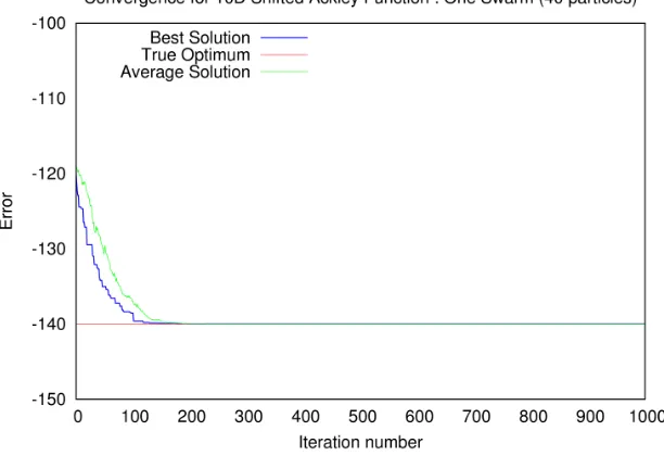
In this section, we observe convergence performance of particle swarm optimization during a typical trial showing the average solution of each particle as well as the best solution in the swarm. For all scenarios, we observe the performance obtained using a single swarm of 40 particles.
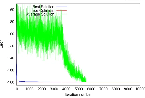
Figure 6.8 shows the convergence pattern for the 10 dimensional (10D) Shifted Sphere function. The blue line tracks the best particle (best solution) at each iteration, green line shows the average solution of all particles at every iteration and the red line shows the global optimum (objective function value). It can be observed that the average solution converges towards the best solution as iterations progress.
Figure 6.8: Shifted Sphere function: Convergence pattern of a typical swarm
Figure 6.9: Shifted Rosenbrock’s function: Convergence pattern of a typical swarm
Figure 6.10: Shifted Rastrigin’s function: Convergence pattern of a typical swarm
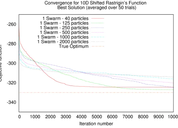
problem to optimize and a single swarm of 40 particles does not converge to the global optimum. The swarm becomes trapped in a local minimum. As we can see from Figure 6.3, Shifted Rastrigin’s function is highly multi-modal and has numerous local minima.
Figure 6.11: Shifted Rastrigin’s function: Convergence pattern of a larger swarm compared to baseline swarm
Figure 6.13 shows the convergence of a typical swarm of 40 particle for the 10D Shifted Schwefel’s function.
Figure 6.13: Shifted Schwefel’s function: Convergence pattern of a typical swarm
Figure 6.14 shows the convergence of a typical swarm of 40 particle for the 10D Shifted Griewank function. Similar to the Shifted Rastrigin’s scenario, convergence is improved when we utilize multiple swarms (4 swarms) for the Shifted Griewank function (see Figure 6.15).
Figure 6.14: Shifted Griewank function: Convergence pattern of a typical swarm
Figure 6.16: Shifted Ackley’s function: Convergence pattern of a typical swarm
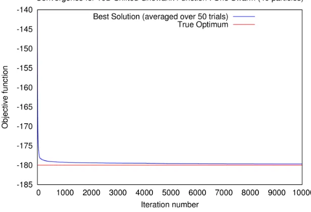
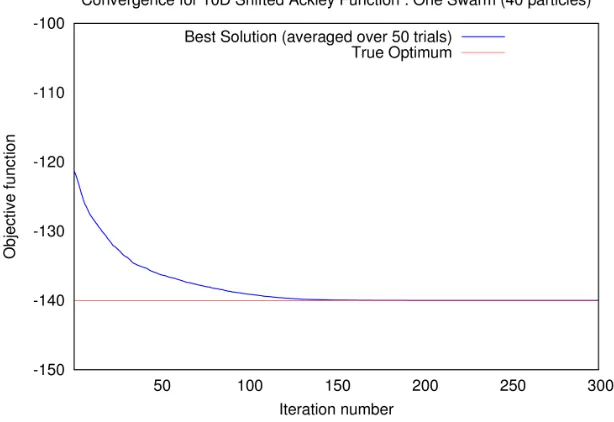
6.2.2
Single Swarm Performance: Robustness
Since PSO is a heuristic search method, it is important to assess the robustness of its efficacy on a test problem over multiple trials. So we ran 50 trials of the aforementioned test problems and plotted the average of the best solution obtained at each iteration across those 50 trials.
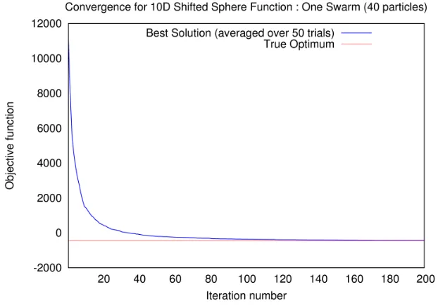
Figure 6.17 illustrates the average performance of PSO using a single swarm for the Shifted Sphere function.
Figure 6.18 illustrates the average performance of PSO using a single swarm for the Shifted Rosenbrock’s function.