Semiparametric Regression and Machine Learning Methods for Estimating Optimal Dynamic Treatment Regimes.

(1)

Semiparametric Regression and Machine Learning

Methods for Estimating Optimal Dynamic

Treatment Regimes

by Yebin Tao

A dissertation submitted in partial fulfillment of the requirements for the degree of

Doctor of Philosophy (Biostatistics)

in The University of Michigan 2016

Doctoral Committee:

Associate Professor Lu Wang, Chair Associate Professor Janis M. Miller Professor Bhramar Mukherjee

(2)

c

(3)

(4)

ACKNOWLEDGEMENTS

This dissertation is an epitome of my five wonderful years at Michigan, full of wis-dom, support and encouragement from my instructors, colleagues, friends and family. Those listed below are a subset, and I apologize to anyone left out.

My sincere gratitude goes to my advisor Dr. Lu Wang. I have been fortunate enough to have Lu guide me through my studies and my life at Michigan. I have enjoyed every single meeting with her, no matter when having breakthroughs or being stuck in some research problems. This dissertation could never be finished without her instruction, inspiration and encouragement. Lu’s approach to always give the right amount of guidance while leaving enough space for my own development has benefited me greatly. I will continue learning from her as I move on to the next phase of my life.

Special thanks go to my other committee members. Janis is a delight to work with. I am deeply grateful to her for helping me improve my collaboration skills with clinical researchers and fit into the academic life in the US shortly after I came here. I cannot thank Bhramar enough for believing in me, and supporting me both intellectually and financially. Her comprehensive knowledge and exceptional multi-tasking ability have been a great inspiration to me. I would not have gone this far without her guidance and support during the first half of my life at Michigan. I must also thank Matt for supporting me during my PhD studies and it is my great pleasure to work with him. I have learned so much from him given his excellent abilities as an applied statistician

(5)

working with medical researchers.

I am grateful to Dr. Wei Huang, my advisor at Peking University, for guiding me into the field of public health and biostatistics. My thanks also go to Dr. Brisa S´anchez for helping me with my research during the MS program. I am thankful to all the knowledgeable faculty members at Michigan for their excellent lectures.

Last but not least, I would like to thank my friends and family, who have made my life so enjoyable. I am especially grateful to my father Weirong Tao, my mother Xueya Huang, and my grandma Aigen Hu for their unconditional love and support, and for making me a better person.

(6)

LIST OF FIGURES

Figure

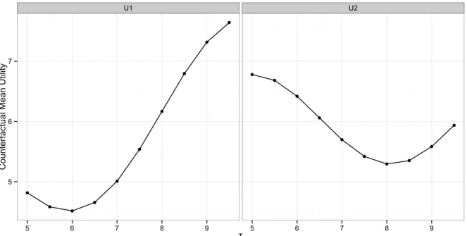
2.1 Counterfactual mean utility for the 10 regimes in simulations with various thresholds τ given utility function U1 (left) or U2 (right). Each point in the plots is calculated from 1000 Monte Carlo samples. 21 2.2 The estimated counterfactual mean utility for dynamic treatment

regimes with various HbA1c thresholds to initiate insulin therapy for the diabetes example. . . 27

3.1 Predicted optimal treatments in simulation Scenario 2 of Chapter III with a tree-type underlying optimal DTR, correctly specified propen-sity score model and sample size of 1000. The true regions at stage 1 are red for X1 > −1 and X2 > 0.5, green for X1 > −1 and −0.5 < X2 ≤ 0.5 and black elsewhere. The true regions at stage 2 are red for R1 > 3 and X3 > −1, green for 0.5 < R1 ≤ 3 and

X3 >−1 and black elsewhere. . . 50 3.2 Predicted optimal treatments in simulation Scenario 2 of Chapter

III with a non-tree-type underlying optimal DTR, correctly specified propensity score model and sample size of 1000. The true regions at stage 1 are red for X1 > 0 and X1 > X2, black for X1 ≤ 0 and green elsewhere. The true regions at stage 2 are red for X3 >0 and

R1 +X3 > 2.5, black for X3 ≤ 0 and R1 +X3 ≤ 2.5, and green elsewhere. . . 51 3.3 Two-stage disease management for esophageal cancer patients. . . . 54

4.1 (A) A decision tree for optimal treatment rules and the expected counterfactual outcome by assigning a single best treatment to each node that represents a subset covariate space. (B) Regions divided by the terminal nodes in the decision tree indicating different optimal treatments. . . 68

(9)

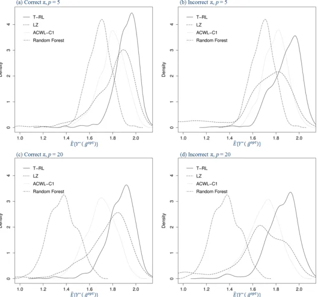
4.2 Density plots for the estimated counterfactual mean outcome in Sce-nario 1 of Chapter IV with varying penalties for misclassification in the generative outcome model (500 replications, n = 500). The four panels are under correctly or incorrectly specified propensity model and five or twenty baseline covariates. . . 78

(10)

LIST OF TABLES

Table

2.1 Estimated counterfactual mean utilityEb(Ug) (empirical SD in

paren-theses) and percentage of replicates selecting g as the optimal DTR (opt%) for regimes in biomarker Scenario 1 of Chapter II. . . 23 2.2 Estimated counterfactual mean utilityEb(Ug) (empirical SD in

paren-theses) and percentage of replicates selecting g as the optimal DTR (opt%) for regimes in biomarker Scenario 2 of Chapter II. . . 24

2.3 Summary statistics (mean±SD) for patients with HbA1c <6.5% at initiation of insulin therapy and those with HbA1c ≥ 6.5% . . . 26

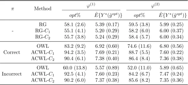
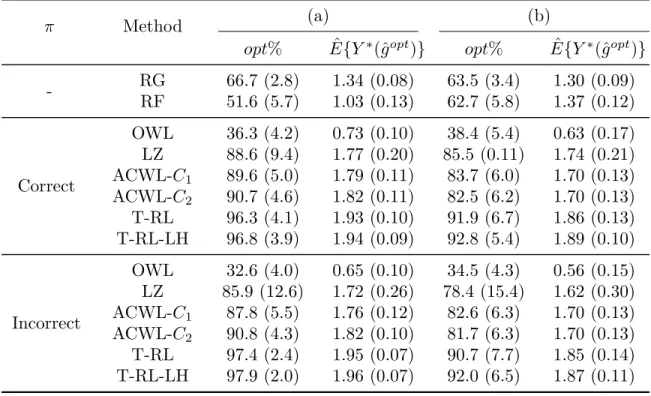
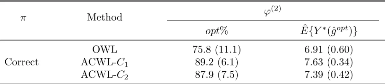
3.1 Simulation results for Scenario 1 in Chapter III with a single stage and five treatment options. π is the propensity score model. ϕ(1)_and _ϕ(2) indicate equal and varying penalties for misclassification. opt% shows the empirical mean and standard deviation (SD) of the percentage of subjects correctly classified to their optimal treatments. ˆE{Y∗(ˆgopt_)} shows the empirical mean and SD of the expected counterfactual outcome obtained using the true outcome model and the estimated optimal regime. E{Y∗(gopt_)}_{= 8, 500 replications, and} _n_{= 1000.} _. ₄₆

3.2 Simulation results for Scenario 2 in Chapter III with two stages and three treatment options at each stage. π is the propensity score model. opt% shows the empirical mean and standard deviation (SD) of the percentage of subjects correctly classified to their optimal treatments. Eˆ{Y∗(ˆgopt_)} _{shows the empirical mean and SD of the} expected counterfactual outcome obtained using the true outcome model and the estimated optimal DTR. E{Y∗(gopt)} = 8, and 500 replications. . . 49

(11)

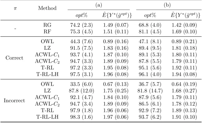
4.1 Simulation results for Scenario 1 in Chapter IV with a single stage, three treatment options and five baseline covariates. π is the propen-sity score model. (a) and (b) indicate equal and varying penalties for treatment misclassification in the generative outcome model. opt% shows the empirical mean and standard deviation (SD) of the per-centage of subjects correctly classified to their optimal treatments.

ˆ

E{Y∗(ˆgopt)}shows the empirical mean and SD of the expected coun-terfactual outcome obtained using the true outcome model and the estimated optimal regime. E{Y∗(gopt)} = 2, 500 replications, and

n= 500. . . 77 4.2 Simulation results for Scenario 1 in Chapter IV with a single stage,

three treatment options and twenty baseline covariates. π is the propensity score model. (a) and (b) indicate equal and varying penal-ties for treatment misclassification in the generative outcome model.

opt% shows the empirical mean and standard deviation (SD) of the percentage of subjects correctly classified to their optimal treatments.

ˆ

E{Y∗(ˆgopt)}shows the empirical mean and SD of the expected coun-terfactual outcome obtained using the true outcome model and the estimated optimal regime. E{Y∗(gopt_)} _{= 2, 500 replications, and}

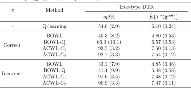
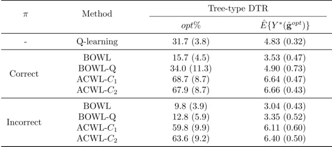
n= 500. . . 79 4.3 Simulation results for Scenario 2 in Chapter IV with two stages and

three treatment options at each stage. π is the propensity score model. opt% shows the empirical mean and standard deviation (SD) of the percentage of subjects correctly classified to their optimal treatments. Eˆ{Y∗(ˆgopt_)} _{shows the empirical mean and SD of the} expected counterfactual outcome obtained using the true outcome model and the estimated optimal DTR. E{Y∗(gopt_)} _{= 8, and 500} replications. . . 83 A.1 Additional simulation results for Scenario 1 in Chapter III with ϕ(2)

and fully randomized treatment assignments. E{Y∗(gopt_)} _{= 8, 500} replications, n= 1000. . . 92 A.2 Additional simulation results based on Scenario 2 in Chapter III,

with treatment assignment models more related to optimal treatment models. E{Y∗(gopt_)}_{= 8, 500 replications,} _n_{= 1000. . . .} ₉₃

A.3 Additional simulation results for two stages and five treatment op-tions at each stage. E{Y∗(gopt_)}_{= 8, 500 replications,} _n_{= 1000. . .} ₉₄

(12)

B.1 Simulation results for a single stage and five treatment options. π is the propensity score model. ϕ(1) _and _ϕ(2) _{indicate equal and} vary-ing penalties for misclassification. opt% shows the empirical mean and standard deviation (SD) of the percentage of subjects correctly classified to their optimal treatments. ˆE{Y∗(ˆgopt_)}_{shows the} empir-ical mean and SD of the expected counterfactual outcome obtained using the true outcome model and the estimated optimal regime.

E{Y∗(gopt_)}_{= 8, 500 replications,} _n_{= 1000. . . .} ₉₇

B.2 Additional simulation results based on Scenario 1 in Chapter IV with five baseline covariates and outcome model indicating arbitrary penalties for misclassification. E{Y∗(gopt)}= 4.69, 500 replications,

n= 500. . . 98 B.3 Additional simulation results based on Scenario 1 in Chapter IV with

five baseline covariates, outcome model (b) and non-tree-type optimal treatment regime. E{Y∗(gopt_)}_{= 2, 500 replications,} _n_{= 500. . . .} ₉₉

(13)

LIST OF APPENDICES

Appendix

A. Supplementary Materials for Chapter III . . . 91

(14)

ABSTRACT

Semiparametric Regression and Machine Learning Methods for Estimating Optimal Dynamic Treatment Regimes

by Yebin Tao

Chair: Associate Professor Lu Wang

Dynamic treatment regimes (DTRs) are sequential decision rules that focus simul-taneously on treatment individualization and adaptation over time. They determine treatment prescriptions based on each individual’s specific characteristics (e.g., demo-graphics, clinical outcomes and genetic makeup) and also adapt the prescriptions over time to evolving illness. We develop robust and flexible semiparametric regression and machine learning methods for estimating optimal DTRs.

In the first project, we consider identifying the optimal personalized timing for treat-ment initiation. Instead of considering multiple fixed decision stages as in most DTR literature, we deal with continuous or multiple random decision points for treatment initiation given each patient’s individual disease and treatment history. For a set of predefined candidate DTRs, we propose to fit a flexible survival model with splines of time-varying covariates to estimate patient-specific probabilities of adherence to each DTR. Given the estimated probabilities, an inverse probability weighted estimator for the counterfactual mean utility (prespecified criteria) is employed to assess each DTR

(15)

and then the optimal one is identified among all candidates. We conduct simulations to demonstrate the performance of our method and further illustrate the application process with an example of insulin therapy initiation among type 2 diabetic patients.

In the second project, we propose a dynamic statistical learning method, adaptive contrast weighted learning (ACWL), which combines doubly robust semiparamet-ric regression estimators with flexible machine learning methods. Compared to the method in Project 1, ACWL can handle multiple treatments at each stage and does not require prespecifying candidate DTRs, despite being limited to a fixed number of treatment stages. At each stage, we develop robust semiparametric regression-based contrasts with the adaptation of treatment effect ordering for each patient, and the adaptive contrasts simplify the problem of optimization with multiple treatment comparisons to a weighted classification problem that can be solved using existing machine learning techniques. The algorithm is implemented recursively using back-ward induction. Through simulation studies, we show that the proposed method is robust and efficient for the identification of the optimal DTR. We further illustrate our method using observational data on esophageal cancer.

In the third project, we propose a tree-based reinforcement learning (T-RL) method to directly estimate optimal DTRs in a multi-stage multi-treatment setting. At each stage, T-RL builds an unsupervised decision tree that maintains the nature of batch-mode reinforcement learning. Unlike ACWL, T-RL handles directly the problem of optimization with multiple treatment comparisons, through the purity measure con-structed with augmented inverse probability weighted estimators. For the multiple stages, the algorithm is implemented recursively using backward induction. By com-bining robust semiparametric regression with flexible tree-based learning, we show that T-RL is robust, efficient and easy to interpret for the identification of optimal DTRs. We illustrate our method in a case study to identify dynamic substance abuse

(16)

(17)

CHAPTER I

Introduction

As the importance of personalized medicine becomes more and more widely recognized in today’s health care, a lot of research efforts are being made in the development of individualized treatment strategies, which are decision rules that dictate what treat-ment to provide given a patient’s specific characteristics (e.g., demographics, clin-ical outcomes and genetic makeup). Dynamic treatment regimes (DTRs) (Robins, 1986, 1997, 2004; Murphy, 2003) mathematically generalize personalized medicine to a time-varying treatment setting, and focus simultaneously on treatment individual-ization and adaptation over time. Identifying optimal DTRs offers an effective vehicle for personalized management of diseases, and helps physicians tailor the treatment strategies dynamically and individually based on clinical evidence, which provides a key foundation for better chronic care (Wagner et al., 2001).

In this dissertation, we consider estimating optimal DTRs, which is difficult due to the complex relationships between the alternating sequences of time-varying treat-ments and clinical outcomes. Standard regression methods fail without being able to adjust for time-varying confounding. The most popular methods for estimating optimal DTRs include marginal structural models (MSMs) with inverse probability weighting (IPW) (Robins, 2000;Hern´an et al., 2001;Wang et al., 2012), G-estimation of structural nested mean models (Robins, 1986, 1989, 1997), generalized by Murphy

(18)

(2003) and Robins (2004), targeted maximum likelihood estimation (van der Laan and Rubin, 2006), and likelihood-based approaches (Thall et al., 2007). Machine learning methods have become popular alternative approaches on estimating optimal DTRs, for example, Q-learning (Watkins and Dayan, 1992; Sutton and Barto, 1998) and A-learning (Murphy, 2003; Schulte et al., 2014), both of which use backward induction (Bather, 2000) to first optimize the treatment at the last stage and then sequentially optimize the treatment at each of the earlier stages.

A DTR is essentially a multi-stage decision problem with two or more options at each stage. It has been developed upon the simplest case of single-stage decision-making with binary treatment options, the so-called individualized treatment regime (Zhang et al., 2012b,a; Zhao et al., 2012; Zhou et al., 2015). Other studies have extended the exploration into multiple treatment stages (Murphy, 2003; Zhang et al., 2013;

Zhao et al., 2015) or multiple treatment options (Laber and Zhao, 2015). We aim to continue this endeavor into more decision stages and/or more treatment options, using flexible and robust methods. In this dissertation, we utilize the counterfactual framework for causal inference (Robins, 1986) to identify the optimal DTR, which means that the optimal DTR would optimize the expectation of a counterfactual mean outcome/utility.

Our first project as presented in Chapter II takes on the task of handling continuous or multiple random decision points with binary treatment options. It is motivated by the example of type 2 diabetes patients enrolled to initiate insulin therapy. Find-ing the optimal personalized timFind-ing to initiate the therapy is essential to achieve the best balance of treatment effectiveness and risk. In the data example, each type 2 diabetes patient has multiple clinical visits at random time points before treat-ment initiation and the treattreat-ment decisions are made at each clinical visit. With the advance in mobile-health technologies (Free et al., 2013) and wearable

(19)

biosen-sor systems for health monitoring (Gatzoulis and Iakovidis, 2007; Pantelopoulos and Bourbakis, 2010), it is now feasible to obtain biomarker measures, such as blood pres-sure and heart rate, continuously over time, so that continuous treatment decisions can be made. However, most existing methods for identifying optimal DTRs have only considered multiple fixed treatment decision stages or even a single stage and thus cannot deal with continuous or multiple random decision points. We provide a general framework based on MSMs to identify the optimal personalized time for treatment initiation given random or continuous decision points. To utilize MSMs with IPW, one has to prespecify candidate DTRs, for example, defining the struc-ture of the DTR to depend on a small set of covariates and searching over a grid of thresholds of these covariates. In our study, we consider a set of predefined DTRs with each representing a way of timing the treatment initiation based on patients’ up-to-date medical history, such as biomarker trajectories. These candidate DTRs are compared by the expectation of a counterfactual mean utility, which also needs to be predefined.

Instead of focusing on continuous or multiple random stages with binary treatment options, Projects 2 and 3 (Chapters III and IV, respectively) work on multiple treat-ment options in the context of multiple fixed decision stages. The treattreat-ment options can be either multinomial or ordinal. A motivation example is the esophageal cancer data where each patient went through two stages of chemotherapy and radiation ther-apy. The methods in the second and third projects are fundamentally different from the one in the first project. In Projects 2 and 3, we combine robust semiparamet-ric regression with flexible machine learning methods for multi-stage multi-treatment decision-making. The algorithms are implemented recursively from the last stage us-ing backward induction (Bather, 2000). Due to the use of machine learning, there is no need to predefine candidate DTRs.

(20)

The problem of multi-stage decision-making has strong resemblance to reinforcement learning (RL), which is a branch of machine learning (Chakraborty and Moodie, 2013). Unlike supervised learning (SL) (e.g., regression and classification), the desired output value or the optimal decision, known as label, is not observed in RL, and the learn-ing agent has to keep interactlearn-ing with the environment to learn the best policy for decision-making. In a DTR problem, the optimal treatment for each patient at each stage is also not observed and can only be inferred based on observed treatments and outcomes from all subjects. In Chapter III, we develop a dynamic statistical learn-ing method, adaptive contrast weighted learnlearn-ing (ACWL), to directly estimate the optimal DTR through a sequence of weighted classifications. Basically, ACWL trans-forms RL into SL by obtaininglabel from a working semiparametric regression model which estimates the treatment effect ordering for each patient at each stage. ACWL can deal with more than two treatments at each stage due to the use of contrasts with the adaptation of treatment effect ordering. The proposed adaptive contrasts stand for the minimum or maximum expected loss in the outcome given any sub-optimal treatment for each patient, and simplify the problem of optimization with multiple treatment comparisons to a weighted classification problem at each stage.

We show that ACWL is robust and efficient for the identification of the optimal DTR and can be easily implemented using existing regression and classification methods. However, it requires the extra step of transforming RL into SL, which may induce additional uncertainty through the identification of label. It also may not the most efficient method by avoiding multiple treatment comparisons. Therefore in Chapter IV, we propose a tree-based reinforcement learning (T-RL) method to directly handle the problem of optimization with multiple treatment comparisons while maintaining the RL nature of the DTR problem. At each stage, T-RL builds an unsupervised decision trees using a purity measure constructed with augmented inverse probability weighted estimators for all treatment options. T-RL enjoys the advantages of typical

(21)

tree-based methods as being straightforward to understand and interpret, and capable of handling various types of data without distributional assumptions. It is also robust and efficient by combining robust semiparametric regression with flexible tree-based learning. However, for non-tree-type underlying DTRs, ACWL may have better performance with the ability of incorporating non-tree-based classification methods.

(22)

CHAPTER II

Optimizing the Personalized Timing for Treatment

Initiation with Continuous or Multiple Random

Decision Points

2.1 Introduction

Many chronic diseases such as cancer and diabetes are of long duration and progres-sive nature. Therefore, long-term health monitoring and dynamic treatment processes with sequential intensification are necessary for patients with such diseases. An im-portant but challenging problem is to find the optimal personalized timing to initiate a treatment for the next stage of disease condition. For example, patients diagnosed with type 2 diabetes usually start with oral anti-diabetic medications, such as met-formin (Glucophage), and their glycated hemoglobin (HbA1c) levels are constantly checked during their regular clinical visits. According to the American Diabetes As-sociation, a reasonable HbA1c goal for many non-pregnant adults is<7% (American Diabetes Association, 2014). As the disease progresses, most patients eventually re-quire and benefit from insulin therapy (Turner et al., 1999). Delayed insulin therapy has been found related to reduced life expectancy and increased risk of microvas-cular and macrovasmicrovas-cular complications (Goodall et al., 2009). However, intensive

(23)

glucose control (e.g., targeting HbA1c < 6%) is rarely effective in achieving tight glycemic control (Hayward et al., 1997) and is associated with adverse effects such as hypoglycemia and weight gain (Gerstein et al., 2008; Patel et al., 2008). There-fore, finding the optimal timing to initiate insulin therapy is essential to achieve the best balance of treatment effectiveness and risk. In most observational data, patients with chronic diseases have their own schedules for examinations of clinical biomarkers (e.g., HbA1c) and their physicians make treatment decisions each time the biomark-ers are measured. The frequency of clinical visits can be considered as a random variable which likely depends on a patient’s disease progression, physical status and the physician’s personal judgment, and the clinical visits are in fact multiple random decision points for treatment decisions. Moreover, with the advance in mobile-health technologies (Free et al., 2013) and wearable biosensor systems for health monitoring (Gatzoulis and Iakovidis, 2007;Pantelopoulos and Bourbakis, 2010), it is now feasible to obtain some biomarker measures (e.g., blood pressure and heart rate) continuously over time, so that continuous treatment decisions, which are more timely and precise, can be made.

Motivated by these examples, we consider a situation where key biomarkers of dis-ease severity are monitored at continuous or multiple random time points during a follow-up period and each time the biomarkers are measured, a decision on treatment initiation is made based on the patient’s up-to-date biomarker and treatment history. Hence, personalized decisions on treatment initiation are made dynamically over time. Regardless of continuous or multiple random visits, the time for each clinical visit can be considered as a continuous random variable from a population perspective. The difference is that with multiple random visits, the biomarker trajectories are not fully observed and we may have to extrapolate using parametric or nonparametric meth-ods. Our goal is to find the optimal timing for treatment initiation given a patient’s biomarker and treatment history. This can be framed as a specific type of dynamic

(24)

treatment regimes (DTRs) (Robins, 1986, 1997, 2004;Murphy, 2003). Instead of hav-ing multiple fixed stages of treatment decisions as in most DTR literature, we consider continuous or multiple random decision points for treatment initiation according to a patient’s up-to-date medical history. Identifying such optimal DTRs offers an effec-tive vehicle for personalized management of diseases, and helps physicians tailor the treatment strategies dynamically and individually based on clinical evidence, which provides a key foundation for better chronic care (Wagner et al., 2001).

Many recent studies have explored the designs of sequential multiple assignment ran-domized trials (SMARTs) (Murphy, 2005) that aim at evaluating DTRs, as well as analytic tools to estimate the effects of DTRs using longitudinal observational or ex-perimental data, as reviewed inWang et al.(2012). Although SMARTs are desirable for causal inference, the more common source of data for constructing DTRs is obser-vational studies. A lot of statistical research has focused on dealing with obserobser-vational data (Murphy, 2003; Robins, 2004; Henderson et al., 2010), where careful thoughts and assumptions are required in order to make valid inference (Robins and Hern´an, 2009). Diverse statistical methods have been developed including G-estimation of structural nested mean models (SNMMs) (Robins, 1986, 1989, 1997), generalized by

Murphy (2003) and Robins (2004), marginal structural models (MSMs) with inverse probability weighting (IPW) (Robins, 2000; Hern´an et al., 2001), targeted maximum likelihood estimators (van der Laan and Rubin, 2006), Q- and A-learning (Watkins and Dayan, 1992; Robins, 2004; Murphy, 2005;Huang and Ning, 2012;Moodie et al., 2012;Chakraborty and Moodie, 2013;Schulte et al., 2014), outcome weighted learning and classification-based methods (Zhang et al., 2012a;Zhao et al., 2012, 2015). How-ever, susceptibility to model misspecification remains as a major limitation of many methods in this field and the computational burden would increase as the number of decision stages increases. Moreover, for methods that rely on backward induction (Bather, 2000), one needs to line up the treatment stages to a finite number. Thus

(25)

most existing studies have only considered multiple fixed treatment decision stages or even a single stage for decision making. Very few attempts exist to handle continuous decision points. For example,Lok (2008) provides a conceptual framework and math-ematical formalization of SNMs in continuous time. However, real data application of their SNMMs based method is still limited to a finite number of stages (Lok and DeGruttola, 2012). Johnson and Tsiatis (2005) consider the duration-response rela-tionship with treatment duration being a continuous random variable, and they apply MSMs to estimate the optimal regimes that are determined solely by the treatment duration.

We aim to provide a general framework based on MSMs to identify the optimal personalized time for treatment initiation given random or continuous decision points, which also applies to dynamic decisions on binary and monotonic treatment switch. We compare a set of predefined DTRs with each representing a way of timing the treatment initiation based on patients’ up-to-date medical history, such as biomarker trajectories. The cause of continuous or random decision points under this framework is that the biomarkers are measured continuously over time or at multiple randomly time points and decisions are made each time the biomarkers are measured. In the type 2 diabetes example, if we consider the timing by the HbA1c level, a possible DTR could be that we initiate insulin therapy only when a patient’s HbA1c level is between 6 ∼ 6.5%. In this case, decisions for treatment initiation are made continuously based on the HbA1c trajectories. Furthermore, under each DTR, instead of modeling directly the time from enrollment to treatment initiation, we focus on the duration when a patient adheres to a given regime. The adherence duration, as a function of the biomarker trajectories and the definition of the DTR, is a continuous random variable specific to a given regime. Most MSMs based methods are limited to a finite number of aligned stages so that one can apply pooled logistic regression to estimate probabilities of adherence to a given DTR at all stages (Robins et al., 2000; Hern´an

(26)

et al., 2001). It is nontrivial to extend this problem to accommodate continuous or multiple random decision points, considering that as the number of stages goes to infinity, the probabilities estimated by pooled logistic regression may go to zero and no longer work in IPW.

The remainder of this paper is organized as follows. We define the DTRs of interest within the framework of causal inference in Section 2.2 and establish our estimation procedure in Section 2.3. We propose to build a survival model with splines of time-varying covariates to calculate the probability of adherence to a given DTR for all patients, given their own covariate history. This model allows much flexibility on how the the risk of failure to follow a specific regime depends on time-varying biomark-ers. Then we use the estimated probability to construct IPW estimators for the counterfactual mean of the utility of interest (e.g., a prespecified measure balancing treatment efficacy and toxicity). The simulation studies (Section 2.4) bring out the salient features of our proposed method. We further illustrate the application process in Section 2.5, using the example of insulin therapy initiation among type 2 diabetic patients, where we consider a class of DTRs that the patients initiate insulin therapy the first time their HbA1c levels reach a certain threshold. Finally, we conclude with some discussions and suggestions for future studies in Section 2.6.

2.2 Notation and Dynamic Treatment Regimes

Suppose that N patients, a random sample from a large target population, are fol-lowed up for a maximum duration of T∗ since enrollment. For patient i at time t, where i = 1, ..., N and 0 ≤ t ≤ T∗, let Xi(t) denote the time-varying biomarkers and we allow Xi(0) to further include all other baseline covariates. Let Ai(t) denote the treatment prescription that takes the value 1 for starting treatment and 0

(27)

oth-erwise. Our interest is in the optimal timing to initiate treatment and we assume that all patients have the same fixed post-initiation treatment plan during the study period. Let Si denote patient i’s treatment initiation time and Si is considered as administratively censored if no treatment is given during the follow-up period, i.e.,

Si > T∗. Therefore, patient i’s observed follow-up duration for treatment initiation is min(Si, T∗), which we denote as Ti. Notably, Ti is also the patient’s duration of continuous random decisions on treatment initiation. In some cases, a patient could terminate study participation before T∗ without being treated due to uncontrollable factors such as death or simply loss to follow-up. These types of censoring can be incorporated in our method if they are non-informative conditional on the observed data. To simplify the problem, we only consider administrative censoring herein after.

For brevity, we suppress the patient index i in the following text when no confusion exists. Following the convention in the literature, we use overbars to denote the history of variables up to the indexed time, underbars to denote the future of variables from the indexed time, capital letters for random variables or vectors, and small letters for observations of the corresponding random variables. For example, the treatment history up to time t is denoted as A(t) ={A(s) : 0≤s≤t} and a possible observed treatment history is denoted asa(t) with value in the range ofA(t), wherea(t)∈ A(t). We denote the observational data up to timet asO(t) = {A(t−),X(t)}, whereA(t−) is the treatment history up to, but not including, timetandX(t) denotes the covariate history up to time t including baseline covariates X(0).

Since the treatment decisions are made continuously and dynamically based on pa-tients’ own medical history, A(t) depends on A(t−) and X(t). Recursively, the time-dependent biomarkers (e.g., HbA1c and morbidity) are also affected by previous treat-ment decisions and past covariate history, i.e.,X(t) also depends onA(t−) andX(t−). A feasible DTR g = g{t;A(t−),X(t)}: 0≤t≤T∗ is a sequential rule for

(28)

deter-mining the next treatment prescription A(t) at time t. For convention, when t = 0, we let A(0−) = _∅ and X(0) = X(0). We denote the collection of all DTRs g of interest as G and g{t;A(t−),X(t)} is a map

[A(t−),X(t)]→g{t;A(t−),X(t)} ∈ A(t) for any t∈[0, T∗],

which may depend on a patient’s part or all of the recorded treatment history before time t and biomarker information up to time t.

In our study, we consider a set of predefined g’s. The optimal DTR is the one that optimizes the expected utility function if all patients in the population follow this rule, which may be contrary to fact. To assess the causal effect of a specific DTR, we consider the counterfactual framework for causal inference (Robins, 1986). Let

xg₍_t_{) denote the counterfactual} _X_{-history up to time} _t _{(e.g., biomarkers or clinical} outcomes) that would be observed in the world where the patient had followed regime

g. Similarly, let ag₍_t_{) denote the counterfactual} _A_{-history (e.g., treatment, action or} intervention) up to timetthat would be observed in the world in which the patient had followed regime g. To assess the treatment effects of g, we define a utility function

U at the end of the study that depends on both X(T∗) and A(T∗). Without loss of generality, we assume that smaller values of U is preferred. Let Ug denote the counterfactual utility function if all subjects have followed regime g. The optimal DTR is the one that minimizes the expected counterfactual utility function, i.e.,

gopt = argmin_g_∈GE(Ug). (2.1)

Note that the expected utility depends on regime g, while the treatment decision at timetaccording to regimegrecursively depends on the patient’s up-to-date biomarker history X(t). Thus, minimizing E(Ug_{) provides the optimal personalized treatment}

(29)

decisions. Obviously, the utility function is the key to assess and compare various regimes of interest, and one can define the utility function based on the goal of the study. Our method can be applied to any study with a target utility function well defined for every subject, but cannot deal with cases where the utility function may be censored, for example, a time-to-event utility function. In that case, an alternative is to redefine the utility function, such as restricted mean survival time, so as to remove the censoring. Future research on time-to-event utility functions may be of great interest, especially considering that the ultimate goal in many medical studies is to prolong patients’ survival time.

2.3 Estimation of the Optimal Dynamic Treatment Regime

2.3.1 Identifiability of the Counterfactual Mean Utility

Note that in the ideal case, to solve the optimization problem (2.1), we need the counterfactual data under all regimes g ∈ G, which is impractical since each patient can only experience one treatment history. Therefore, instead of using data collected from the counterfactual world as if everyone had followed g, we need to estimate

E(Ug_{) using the observed data} _O₍_T∗_{). In order to do that, we make the following}

three assumptions suggested by previous studies (Murphy et al., 2001; Robins and Hern´an, 2009;Orellana et al., 2010a).

• Consistency assumption: For any regime g, if a given patient has A(t) =

g{t;A(t−),X(t)} for any t ∈[0,˜t], then Xg(˜t) =X(˜t) for any ˜t∈[0, T∗]; and if

A(t) = g{t;A(t−),X(t)}for anyt ∈[0, T∗], thenUg ₌_U _{for that patient. That} is to say, if the actual treatment history observed for a patient is compatible with DTR g, his or her observed biomarker and utility function are the same

(30)

as the counterfactual ones under g.

• No unmeasured confounder assumption (NUCA): NUCA implies that at any

t∈[0, T∗],

A(t)⊥ {Ug,X(t)}|{A(t−),X(t)}

for regime g, where X(t) is the future of variables X starting from time t. In other words, the treatment decision at time t is independent of future observa-tions and the counterfactual outcomes, conditional on {A(t−),X(t)} that are recorded until just prior to assigning A(t).

• Positivity assumption: We assume that at any time t∈[0, T∗],

Pg P rA(t) =g{t;A(t−),X(t)}|A(t−),X(t)>0= 1,

where Pg _{is the law of}_{_A₍_t−₎_,_X₍_t_)} _{in the counterfactual world where regime}

g were enforced for the entire population. This assumption basically guarantees that if in the counterfactual world where everyone followed regimeg, there were patients with historyx(t) and a(t−), then in the observational data among the subjects with the same covariates history x(t) who actually followed regime g

up to time t−, there is a subset who also follow regime g at timet.

With these assumptions, we are able to make inference about E(Ug) using only the observed data (Robins and Hern´an, 2009; Orellana et al., 2010a,b). Specifically, for a DTR g at any t ∈ [0, T∗], we define Cg₍_t_{) =} _I_[_A₍_t_{) =} _g_{_t_;_A₍_t−₎_,_X₍_t_{)}] as the}

indicator of adherence that takes the value 1 if a patient adheres to g at time t

and 0 otherwise. Therefore, if Cg(t) = 1(t), where 1(t) is a function with constant value of 1 up to t, it means that this patient follows g up to t. As defined before, a patient’s decision process for treatment initiation is random till T = min(S, T∗), and thus we assess the patient’s adherence history up to T, i.e., Cg(T). Let Fg

(31)

denote the time to failure of adherence to DTRg and we haveFg ₌_min

t{t∈[0, T] :

Cg₍_t_{) = 0}}_{for a patient whose failure of adherence is observed within}_T_{. On the other} hand, for a patient who follows g all the way to T, whether treated (i.e., T =S) or administratively censored (i.e., T =T∗),Fg _{is not observed and the only information} is Fg _{> T}_{. In other words, the patient’s time to failure of adherence to}_g _{is censored} atT.

Using our notation, only patients with Cg(T) = 1(T) actually follow g for treatment initiation during the study and have Ug _{observed. The observed utility} _U _{of other} patients who have Cg₍_t_{) = 0 for some} _t_∈ _[0_{, T}_{] are actually affected by other} treat-ment assigntreat-ments on and after Fg_{, and thus cannot be used to estimate} _E₍_Ug_{). If} we denote the counterfactual law under DTR g byPg _{and the observational law by}

P, then under Assumptions (1) - (3) we have

dPg dP A(T),X(T) = I Cg(T) = 1(T) P rCg(T) = 1(T)|X(T),

whereI(·) is the indicator function that takes the value 1 if ·is true and 0 otherwise.

In our study, the patients compatible with g have their time to failure of adherence tog censored at T. Therefore, P rCg(T) = 1(T)|X(T) =P rFg > T|X(T). If we define ωg = I C(T) = 1(T) P r Fg _{> T}_|_X₍_T₎,

then under Assumptions (1) - (3),

E(Ug) = E UdP g dP A(T),X(T) =E(U ωg). (2.2)

(32)

Therefore, the bias induced from using the subset of patients who actually follow g

in the observational data can be corrected for by weighting each patient with the corresponding inverse probability of adherence. We apply the IPW method (Murphy et al., 2001; Wang et al., 2012) and estimate E(Ug_{) as the weighted mean of the} observed U among patients adherent to DTRg throughout the study period.

2.3.2 Estimation of the Weights and Counterfactual Mean Utility

We denote πg ₌ _{P r}_[_Fg _{> T}_|_X₍_T_{)], the adherence probability. Then the weight} _ωg for an adherent patient is 1/πg_{, while that of a non-adherent patient is 0. According} to (2.2), the estimation of E(Ug_{) depends on} _ωg _{and equivalently,} _πg_{. Therefore, a} robust estimate of πg is essential to guarantee the validity of Eb(Ug). We propose

a flexible time to failure of adherence model with time-varying biomarkers, which allows both linear terms and flexible spline functions of covariates. Specifically, from the biomarker set X, we select biomarkers XL

l (l = 1, ..., m) as linear terms (e.g., categorical variables) and XS

j(j = 1, ..., k) to be fit in spline terms (e.g., continuous variables with unknown effects on adherence), which can be determined by scientific knowledge related to the study and regime definition. Then the flexible Cox model for the hazard of failing to adhere to DTR g at time t is

λg{t|X(t) = x(t)}=λg₀(t)exp " _m X l=1 β_lgxL_l(t) + k X j=1 f_jgxS_j(t) # (2.3)

where λg₀(t) is an unspecified baseline hazard function, β_lg is an unknown parameter for X_lL, and f_jg(·) is a spline function for X_jS with details given below. Note that we model the hazard at t with only the current biomarker observations, which can be easily extended to include summary variables indicating certain aspects of the covariate history up to t (e.g., percent of time with HbA1c over 8% from enrollment

(33)

to t). For convenience, we write all covariates in the time-varying form and simply let baseline covariates to be constant over time. The parameterization used for the splines is f_jg(x) = M+3 X h=1 θg_jhBjh(x)

where Bjh’s are standard cubic B-spline basis functions (De Boor, 1978), θ g

jh is the parameter corresponding toBjh andM is the number of knots. The constant term is absorbed in the unknown baseline hazard λg₀(t). The function f_jg(·) is only required to be smooth enough to have continuous second derivatives, and is not restricted to any specific parametric form. Therefore, it allows enough flexibility in (2.3) to get a robust estimate of πg_{, the adherence probability. Then we can obtain}

b ωg_{, and} estimate E(Ug_{) consistently with the IPW estimator (}_{Wang et al.}_{, 2012)}

b E(Ug) = Pn i=1ωb g iUi Pn i=1ωb g i . (2.4)

According toRobins (2000), the IPW estimator (2.4) will be consistent if the models for estimating πg, the denominator of ωg, are correctly specified, and furthermore,

b

E(Ug) will be√nconsistent if _bπg converges at a rate ofn1/4 or faster. It implies that our IPW estimator can perform well as long as the adherence probability estimated from model (2.3) is not exceedingly variable. To ensure this, we follow Gray (1992) to use fixed knot splines with a modest number of knots and use penalized partial likelihood to estimate the parameters of model (2.3). To maximize the penalized log-partial likelihood, the smoothing parameters for the penalty terms are solved for by first specifying degrees of freedom for the spline smoothers (Buja et al., 1989; Gray, 1992). We choose the optimal degrees of freedom according to the corrected Akaike information criteria (AIC) of Hurvich et al. (Hurvich et al., 1998). For the baseline hazard, we use the Breslow estimator (Breslow, 1972, 1974), which converges at a

(34)

rate of n1/2 ₍_Tsiatis_{, 1981).}

2.4 Simulations

We conduct simulation studies to evaluate the performance of the proposed method given access to the simulated counterfactual data. For each patient under each defined regime, we simulate the counterfactual biomarkers and utility functions, and calculate the real causal outcome using these data. The proposed method is applied to each simulation scenario and then compared to the truth and several competing methods. Our estimation is based on 500 replicates each with sample size N = 500.

2.4.1 Simulation Settings

For simplicity, we simulate one biomarker X that is linearly increasing before treat-ment initiation over the study period [0, T∗ = 120]. For patient i at visiting time

t (before treatment initiation), we generate the biomarker observation from Xi(t) =

β0i +β1it+ti, where patient-specific intercept β0i and slope β1i are independently drawn from N(2.5,0.52) and N(0.07,0.022), respectively, and measurement error

ti ∼N(0,0.12). We also simulate a binary baseline covariate Zi with success rate of 0.5. We define the DTR g to be initiating treatment when X falls into an interval [τ, τ + 0.5) and basically, a patient fails to follow the regime g if he or she starts treatment with X < τ (too early) or X ≥ τ (too late). We consider ten regimes

g1, g2, . . . , g10 with τ1 = 5.0, τ2 = 5.5, . . . , τ10 = 9.5, respectively. Given Xi(t), we calculate the counterfactual treatment initiation time S_igj (j = 1,2, . . . ,10) had the subject followed gj. We randomly assigned one of the ten regimes to each subject as the true underlying DTR, which is not observed. The observed adherence depends on the biomarker trajectory up to the time of treatment initiation. The observed

(35)

decision period for patient i with underlying DTR g is T_ig = min{S_ig, T∗}. Appar-ently, whether or not a patient is administratively censoring is jointly determined by

T∗,X andg. An administratively censored patient may be compatible with multiple regimes. For example, a patient with X increasing from 4.0 at baseline to 6.2 at T∗

without treatment is compatible with regimes that have τ >6.2, i.e., g4, . . . , g10.

In the ideal case, we need all patients’ biomarkers fully observed throughout the study to apply the survival model (2.3). However, in practice, we oftentimes only observe

X at a limited number of clinical visits. Moreover, patients with worse conditions tend to have more clinical visits. To investigate how this can affect our selection of the optimal DTR, we create two biomarker scenarios:

• In Scenario 1, we have access to biomarker observations at each event time (i.e., the time one or more patients fail to followg) for patients at risk (i.e., adherent tog and untreated before).

• In Scenario 2, patient i has X observed at enrollment and Ti (i.e., time of treatment initiation or end of study), and the number of visits in-between follows

binomial(d0.1Tie, ρi), whered·e means taking the smallest integer not less than ·andρi = 1/[1 +exp(1−0.3β0i−10β1i+ 0.2Zi)]. The time of each visit between enrollment andTi is uniformly sampled from (0, Ti).

Scenario 1 provides the whole biomarker history needed for the estimation of the adherence model (2.3) (e.g., the case of mobile medicine). Scenario 2 is to mimic a more common situation with longitudinal biomarker measurements at random clinical visits. We let ρ depend on X and Z in a way that subjects with larger X and smaller Z are expected to have more clinical visits. We extrapolate the values of X

between visits for model (2.3). For example, one can fit a linear mixed model for the trajectories using polynomial terms for t and make patient-specific predictions for

(36)

X. However, in the case of informative observation times, further adjustments may be necessary to correct for bias (Sun et al., 2005, 2007). Another simpler method is to conduct patient-specific extrapolation without borrowing information from other subjects. In our simulations, we use linear extrapolation to estimate the biomarker value at a given event time for each patient still adherent to g.

Our utility function applies to both treated and administratively censored patients. Specifically, for subject i following g with threshold τ, we have

U_ig =      70β1i+ei if administratively censored 0.5τ + 70β1i ·φ(τ) +ei if treated

whereei ∼N(0,0.12). Note that the utility function depends on both the slope of the biomarker trajectory and the DTR. We consider two utility functions with different

φ(τ): U1 with φ(τ) = 0.6 + 0.3cos(0.8τ −2), which is minimized at τ = 6.0, and

U2 withφ(τ) = 0.6 + 0.3cos(0.8τ −3.6), which is minimized at τ = 8.0, as shown in Figure 2.1. These two functions correspond to two situations where treatments are more effective at earlier and later stages of disease, respectively. Furthermore, in our simulation setting, all DTRs have a similar number of treated compatible patients (∼ 50). However, regimes with smaller thresholds have a much lower percentage of administrative censoring among their compatible patients (range: ∼ 5% for τ1 to ∼ 60% for τ10), and thus we are also able to investigate how various percentages of censoring would affect the detection of the optimal regime. We use U1 and U2 in both biomarker scenarios.

For comparison, we consider the unweighted method, simply averaging the observed utility of all patients compatible with the regime of interest, as well as the weighted method with weights from two types of pooled logistic regression (Robins et al., 2000;

(37)

U1 U2 5 6 7 5 6 7 8 9 5 6 7 8 9 τ C ou nt erf act ua l Me an U til ity

Figure 2.1: Counterfactual mean utility for the 10 regimes in simulations with various thresholds τ given utility function U1 (left) or U2 (right). Each point in the plots is calculated from 1000 Monte Carlo samples.

X, denoted as PPL, while the second one applies generalized additive model (GAM) with smoothing splines for X, denoted as NPL. Since time to failure of adherence is continuous, we discretize the period into five intervals by quintiles of event time and apply logistic regression within each interval. We use the biomarker observations in each interval as the one at event time for a patient who fails in that interval, or the one linearly extrapolated at the center of that interval for a patients who is still adherent.

2.4.2 Simulation Results

Table 2.1 summarizes the performance of all methods in evaluating the ten regimes in biomarker Scenario 1, in term of estimated counterfactual mean utility functionEb(Ug)

and the percentage of replicates selecting g as the optimal DTR (opt%). Generally, the weighted methods are far superior to the unweighted one. With U1 where the

(38)

optimal DTR has τ = 6, all weighted methods have very accurate selection of the optimal regime (> 95%) and our proposed method is only slightly better. The two pooled logistic methods are almost identical in selection ofgopt _{and NPL has slightly} smaller bias and variance in Eb(Ug). Comparing the results with the utility function U1 to those withU2, all methods have worse performance. PPL has the largest drop in opt% (from 95.2% to 67.6%) and a wide range of mis-selected regimes. NPL, as a more flexible method than PPL, still has an acceptable performance with 77% of the time selecting the correct optimal DTR and only three different regimes selected. Our proposed method maintains very satisfactory performance with opt% of 94.4%, and much smaller bias and variance in Eb(Ug). From Scenario 1, we can see that our

proposed method can well handle the increased bias due to administrative censoring.

In Table 2.2, we present the results for biomarker Scenario 2, where we extrapo-late the biomarker observations from longitudinal visits. Compared to Scenario 1, all weighted methods have worse performance with the biomarker trajectories only partially observed. Given more uncertainty in the biomarker extrapolation, the bias and variance inEb(Ug) increases and thus more mis-selection has occurred. Note that

results from the full adherent (counterfactual) and the unweighted methods are the same as in Table 2.1 since we use the same simulated samples. In terms of opt%, PPL drops over 20% withU1 from Scenario 1 to Scenario 2, and has only 60.2% correctness with U2 in Scenario 2. NPL is still slightly better than PPL. Our proposed method works much better than the other methods, with about 20% higher chance to select

gopt, smaller bias and variance, and fewer mis-selected regimes. From Scenario 1 to Scenario 2, it only drops less than 10% in opt% and has over 80% correctness withU2 in Scenario 2, which is the most noisy situation. Through the two biomarker scenarios each combined with two different utility functions, we can see that the performance of the proposed method is robust.

(39)

T able 2.1: Estimated coun terfactual mean u tilit y bE ( U g ) (empirical SD in paren theses) and p ercen tage of replicates sele cting g as the optimal DTR (opt%) for regimes in biomark er Scenario 1 of Chapter II. Regime F ull Adheren t Un w eigh ted PPL 1 NPL 2 Prop osed Metho d bE ( U g) opt% bE ( U g) opt% bE ( U g) opt% bE ( U g) opt% bE ( U g) opt% U 1 τ1 = 5 . 0 4.816 (0.032) 0 4.524 (0.154) 0 4.921 (0.221) 0 4.845 (0.133) 0 4.793 (0.143) 0 τ2 = 5 . 5 4.583 (0.028) 0 4.206 (0.162) 0.2 4.492 (0.099) 0.4 4.501 (0.081) 0.2 4.555 (0.071) 0 τ3 = 6 . 0 4.515 (0.027) 100 4.015 (0.160) 47.4 4.373 (0.092) 95.2 4.394 (0.073) 95.4 4.492 (0.062) 97.3 τ4 = 6 . 5 4.655 (0.030) 0 4.014 (0.161) 44.4 4.518 (0.058) 4.4 4.534 (0.069) 4.8 4.594 (0.057) 2.7 τ5 = 7 . 0 5.008 (0.037) 0 4.160 (0.175) 7.6 4.845 (0.076) 0 4.863 (0.072) 0 4.923 (0.068) 0 τ6 = 7 . 5 5.538 (0.047) 0 4.426 (0.211) 0.4 5.334 (0.084) 0 5.352 (0.084) 0 5.417 (0.073) 0 τ7 = 8 . 0 6.168 (0.066) 0 4.735 (0.266) 0 5 .912 (0.119) 0 5.919 (0.110) 0 6.036 (0.089) 0 τ8 = 8 . 5 6.796 (0.088) 0 5.027 (0.274) 0 6 .538 (0.268) 0 6.509 (0.139) 0 6.720 (0.125) 0 τ9 = 9 . 0 7.317 (0.110) 0 5.307 (0.360) 0 7 .031 (0.203) 0 7.065 (0.169) 0 7.218 (0.173) 0 τ10 = 9 . 5 7.643 (0.130) 0 5.524 (0.375) 0 7.450 (0.247) 0 7.511 (0.240) 0 7.775 (0.238) 0 U 2 τ1 = 5 . 0 6.780 (0.057) 0 6.320 (0.253) 0 7.022 (0.329) 0 6.845 (0.244) 0 6.648 (0.252) 0 τ2 = 5 . 5 6.683 (0.055) 0 6.050 (0.283) 0 6.497 (0.213) 0 6.516 (0.172) 0 6.624 (0.127) 0 τ3 = 6 . 0 6.419 (0.052) 0 5.572 (0.278) 0 6.087 (0.379) 1.0 6.165 (0.161) 0 6.235 (0.118) 0 τ4 = 6 . 5 6.060 (0.049) 0 5.084 (0.246) 0 5.804 (0.113) 0.4 5.839 (0.120) 0 5.925 (0.083) 0 τ5 = 7 . 0 5.698 (0.048) 0 4.642 (0.216) 0.4 5.471 (0.104) 0.2 5.499 (0.099) 0 5.654 (0.071) 0 τ6 = 7 . 5 5.420 (0.045) 0 4.349 (0.203) 8.0 5.223 (0.080) 2.4 5.239 (0.080) 2.0 5.387 (0.060) 0.8 τ7 = 8 . 0 5.294 (0.049) 100 4.204 (0.203) 37.2 5.120 (0.091) 67.6 5.122 (0.083) 77.2 5.231 (0.063) 92.2 τ8 = 8 . 5 5.351 (0.055) 0 4.197 (0.180) 39.0 5.203 (0.178) 28.0 5.182 (0.087) 20.8 5.293 (0.079) 7.0 τ9 = 9 . 0 5.584 (0.065) 0 4.331 (0.227) 12.8 5.425 (0.120) 0.4 5.445 (0.103) 0 5.496 (0.096) 0 τ10 = 9 . 5 5.937 (0.080) 0 4.555 (0.242) 2.6 5.826 (0.158) 0 5.853 (0.128) 0 6.023 (0.129) 0 1PPL: p o oled logistic m etho d with parametric terms for biomark ers. 2NPL: p o oled logistic metho d with smo othing splines (GAM) for biomark ers.

(40)

T able 2.2: Estimated coun terfactual mean u tilit y bE ( U g ) (empirical SD in paren theses) and p ercen tage of replicates sele cting g as the optimal DTR (opt%) for regimes in biomark er Scenario 2 of Chapter II. Regime F ull Adheren t Un w eigh ted PPL 1 NPL 2 Prop osed Metho d bE ( U g) opt% bE ( U g) opt% bE ( U g) opt% bE ( U g) opt% bE ( U g) opt% U 1 τ1 = 5 . 0 4.816 (0.032) 0 4.524 (0.154) 0 4.774 (0.186) 1.2 4.778 (0.123) 0 4.780 (0.144) 0 τ2 = 5 . 5 4.583 (0.028) 0 4.206 (0.162) 0.2 4.625 (0.191) 8.9 4.610 (0.125) 2.3 4.690 (0.108) 1.0 τ3 = 6 . 0 4.515 (0.027) 100 4.015 (0.160) 47.4 4.361 (0.225) 70.2 4.401 (0.106) 75.3 4.492 (0.084) 90.2 τ4 = 6 . 5 4.655 (0.030) 0 4.014 (0.161) 44.4 4.482 (0.262) 18.8 4.510 (0.093) 21.0 4.582 (0.071) 8.8 τ5 = 7 . 0 5.008 (0.037) 0 4.160 (0.175) 7.6 4.800 (0.110) 0.9 4.795 (0.101) 0.4 4.901 (0.079) 0 τ6 = 7 . 5 5.538 (0.047) 0 4.426 (0.211) 0.4 5.203 (0.118) 0 5.200 (0.107) 0 5.348 (0.092) 0 τ7 = 8 . 0 6.168 (0.066) 0 4.735 (0.266) 0 5 .680 (0.152) 0 5.677 (0.139) 0 6.032 (0.101) 0 τ8 = 8 . 5 6.796 (0.088) 0 5.027 (0.274) 0 6 .142 (0.184) 0 6.163 (0.167) 0 6.700 (0.143) 0 τ9 = 9 . 0 7.317 (0.110) 0 5.307 (0.360) 0 6 .612 (0.231) 0 6.670 (0.215) 0 7.220 (0.221) 0 τ10 = 9 . 5 7.643 (0.130) 0 5.524 (0.375) 0 7.030 (0.245) 0 7.120 (0.223) 0 7.785 (0.245) 0 U 2 τ1 = 5 . 0 6.780 (0.057) 0 6.320 (0.253) 0 6.470 (0.346) 0 6.491 (0.300) 0 6.452 (0.254) 0 τ2 = 5 . 5 6.683 (0.055) 0 6.050 (0.283) 0 6.335 (0.375) 0 6.467 (0.290) 0 6.816 (0.137) 0 τ3 = 6 . 0 6.419 (0.052) 0 5.572 (0.278) 0 6.045 (0.400) 2.4 6.101 (0.158) 0 6.246 (0.125) 0 τ4 = 6 . 5 6.060 (0.049) 0 5.084 (0.246) 0 5.761 (0.292) 2.0 5.765 (0.138) 0 5.910 (0.107) 0 τ5 = 7 . 0 5.698 (0.048) 0 4.642 (0.216) 0.4 5.431 (0.166) 3.4 5.424 (0.121) 0.5 5.589 (0.094) 0 τ6 = 7 . 5 5.420 (0.045) 0 4.349 (0.203) 8.0 5.110 (0.117) 5.8 5.116 (0.113) 7.1 5.310 (0.080) 1.8 τ7 = 8 . 0 5.294 (0.049) 100 4.204 (0.203) 37.2 4.982 (0.107) 60.2 4.983 (0.100) 64.9 5.200 (0.085) 83.0 τ8 = 8 . 5 5.351 (0.055) 0 4.197 (0.180) 39.0 5.016 (0.117) 25.7 5.029 (0.107) 27.0 5.266 (0.090) 15.2 τ9 = 9 . 0 5.584 (0.065) 0 4.331 (0.227) 12.8 5.244 (0.128) 0.5 5.286 (0.118) 0.5 5.473 (0.107) 0 τ10 = 9 . 5 5.937 (0.080) 0 4.555 (0.242) 2.6 5.660 (0.155) 0 5.703 (0.139) 0 5.913 (0.144) 0 1PPL: p o oled logistic m etho d with parametric terms for biomark ers. 2NPL: p o oled logistic metho d with smo othing splines (GAM) for biomark ers.

(41)

2.5 Application to Diabetes Example

In this section, we applied the proposed method to Eli Lilly’s diabetes electronic medical record (EMR) database from Humedica. We considered patients with only type 2 diabetes, without diagnosis of type 1 or gestational diabetes, and our data was recorded from January 1, 2005 to December 31, 2010. All patients had baseline age and body mass index (BMI) measured at their first clinical visit, and during the follow-up period, their HbA1c level, use of oral anti-diabetic drugs, hospitalizations and comorbidities were recorded at several random visits (range of visiting times: 4∼ 68). HbA1c is the primary biomarker tested for diabetes management and research, as well as for initiating insulin therapy (Hayward et al., 1997). Our goal is to use DTRs to identify the best timing to initiate insulin therapy based on patients’ HbA1c levels.

We defined viable DTRs as initiating insulin therapy when a patient’s HbA1c level is observed to be in an interval [τ, τ + 0.5), similar to the definition in simulations. In other words, a patient fails to follow a given DTR if he or she starts insulin therapy with HbA1c measurement < τ during the same clinical visit or does not start with HbA1c measurement≥τ+ 0.5. We considered the threshold τ from 5.5 to 8.5% with an increment of 0.5%. To be included in our analysis, each patient must have at least two clinical visits before insulin treatment and baseline HbA1c level lower than 10%, resulting in a cohort of 1220 patients. The patients are mostly seniors with obesity (BMI>30). Table 2.3 compares patients with HbA1c <6.5% and those with HbA1c ≥6.5% at treatment initiation. The two groups are very similar in all aspects except HbA1c. The group with lower HbA1c at treatment initiation also has lower HbA1c at enrollment and at the end of study. However, its average HbA1c increases from 6.3 to 6.8% while in the other group, the average HbA1c decreases from 7.8 to 7.7%. Given the variables available in our data, we defined a utility function for each patient as

(42)

Table 2.3:Summary statistics (mean ± SD) for patients with HbA1c < 6.5% at initi-ation of insulin therapy and those with HbA1c ≥ 6.5%

Variable HbA1c at Initiation of Insulin Therapy

<6.5% (n= 162) ≥6.5% (n= 1058)

Age (yrs) 63.5±8.6 63.0±8.4

BMI 34.6±6.7 34.7±7.5

Anti-diabetic drugs before insulin (frequency) 0.6±0.9 0.7±1.1

New complications at end of study (type) 4.1±2.4 4.0±2.3

Hospitalizations at end of study (frequency) 1.5±5.6 1.4±3.8

HbA1c at baseline (%) 6.3±0.7 7.8±1.0

HbA1c at end of study (%) 6.8±1.1 7.7±1.4

the sum of two relative levels. The first one is relative HbA1c level calculated as the mean HbA1c level during follow-up divided by the diagnosis threshold of 6.5%. The second one is relative morbidity level calculated as the total number of new diseases developed during follow-up divided by four which is the median in this database. With this utility function, we aim to find the optimal DTR that controls both glycemic level and comorbidities that come either as side effects of insulin therapy or from diabetes progression. We applied the survival model (2.3) to estimate the weights. As in simulation Scenario 2, we used linear extrapolation to estimate the biomarker value at the event time for patients at risk. We used cubic B-splines for time-varying HbA1c observations and linear terms for all other covariates.

Figure 2.2 presents the estimated counterfactual mean utility for each of the regimes of interest. The number of compatible patients ranges from 32 to 251 for different regimes. The regime with HbA1c threshold of 6.0% has the minimal estimated coun-terfactual mean utility and thus is identified asgopt _{by our proposed method. It means} that initiation of insulin treatment for diabetic patients with HbA1c level of 6∼6.5% may lead to the best overall control of diabetes severity and related comorbidities. However, this result might be sensitive to the choice of the utility function.

(43)

1.5 2.0 2.5 3.0 5.5 6.0 6.5 7.0 7.5 8.0 8.5 HbA1c Threshold (%) Counterf

actual Mean Utility

Figure 2.2: The estimated counterfactual mean utility for dynamic treatment regimes with various HbA1c thresholds to initiate insulin therapy for the diabetes example.

(44)

2.6 Discussion

In this article, we address the challenge of estimating the optimal DTR for treatment initiation given continuous random decision points based on patients’ up-to-date clin-ical records. Our proposed method successfully fills the gap in DTR literature where most existing studies have only considered several fixed stages of treatment decisions. Compared to existing methods, the proposed method has multiple strengths. First of all, it makes minimal model assumptions and is more robust to model misspecifica-tion. Our assumption is primarily made on estimating πg _{through adherence model} (2.3), and the use of splines allows much flexibility on how the risk of failure to fol-low a specific regime depends on time-varying biomarkers. In contrast, the pooled logistic regression requires assumptions about the treatment models at every stage, and Q- and A-learning methods both require assumptions about the structure on the outcome and treatment models at every stage, resulting in high susceptibility to model misspecification. Furthermore, with one adherence model (2.3) for each DTR g regardless of the number of decision points, our method is more stable, com-pared to pooled logistic regression, and more computationally feasible, comcom-pared to Q- and A-learning methods. As the number of stages increase, the weights derived from pooled logistic regression may become very unstable if, for example, there are very few events at a certain stage, leading to both bias and imprecision (Robins and Hern´an, 2009). Q- and A-learning methods use backward recursive fitting procedure (Bather, 2000), and as the number of stages increases, the computational burden may increase dramatically.

The proposed method can be used for many types of DTRs with multiple random decision points, not limited to the problem of treatment initiation. The key is to prespecify a class of meaningful candidate DTRs and build an appropriate model to estimate the probability of adherence to each DTR. For a time to failure of adherence

(45)

model like model (2.3), there should be enough biomarker observations at different decision points and the time to failure of adherence should be a continuous random variable. In order to assess adherence, the treatment decision rules should be clearly defined and consistent throughout the study period.

Several improvements and extensions can be explored in future studies given the re-strictions in our method. First, more flexible methods can be considered for robust weight estimation, for example, the random survival forest (Ishwaran et al., 2008).

Bou-Hamad et al. (2011) has extended the method to allow for time-varying covari-ates. However, a more flexible method may have a lower convergence rate and one should proceed carefully considering the sample size. Second, we have only considered a limited number of well defined DTRs. In practice, there could be a larger or even infinite number of candidate regimes. For example, if we treat the HbA1c thresholds as continuous, we will have an infinite number of regimes. Furthermore, if we have many variables that may affect treatment decisions, we may also end up with a large number of DTRs that deal with various scenarios. Then with a limited sample size, it is impossible to find enough compatible patients for each regime to make inference separately. A feasible solution is to fit a nonsaturated marginal structural model for the utility conditional on the variables that define the DTRs (Robins, 2000; Hern´an et al., 2001). One may also apply classification or machine learning methods to select a subset or some combinations of variables for regime definition so as to reduce the number of DTRs of interest. Third, joint modeling of a multivariate utility function (e.g., toxicity, efficacy and management cost) may be of interest for future research. A univariate utility function is easier for comparison of various DTRs, but its definition may be arbitrary. However, with a multivariate utility function, one needs to search over a multi-dimensional plane to find the optimal DTR that achieves the best joint payoff, which can be computationally complex.

(46)

CHAPTER III

Adaptive Contrast Weighted Learning for

Multi-Stage Multi-Treatment Decision-Making

3.1 Introduction

Individualized treatment strategies (ITS) are decision rules that dictate treatment prescriptions based on a patient’s specific characteristics (e.g., demographics, clinical outcomes and genetic makeup). Given the increasingly popular theme of personalized medicine, many clinical and intervention scientists have now become interested in the development of ITS. Treatment individualization is important due to the fact that many diseases, such as cancer and diabetes, have complex causes by the interplay among genetic, physiological and environmental factors that vary from person to person. The effectiveness of a given treatment is usually determined not only by a patient’s current disease status but also by his/her past treatment and disease history and perhaps other concurrent medical conditions. Moreover, due to the progressive nature of many chronic diseases, treatment adaptation over time is also crucial to optimize treatment effects.

Dynamic treatment regimes (DTRs) (Robins, 1986, 1997, 2004;Murphy, 2003) mathe-matically generalize personalized medicine to a time-varying treatment setting. They