Development of a Decision Support Framework forIntegrated Watershed Water Quality Management and a Generic Genetic Algorithm Based Optimizer

Abstract

PARANDEKAR, AMEY, VIJAY. Development of a Decision Support Framework for Integrated Watershed Water Quality Management and a Generic Genetic Algorithm Based Optimizer. (Under the direction of Dr. S. Ranji Ranjithan.)

The watershed management approach is a framework for addressing water quality problems at a watershed scale in an integrated manner that considers many conflicting issues including cost, environmental impact and equity in evaluating alternative control strategies. This framework enhances the capabilities of current environmental analysis frameworks by the inclusion of additional systems analytic tools such as optimization algorithms that enable efficient search for cost effective control strategies and uncertainty analysis procedures that estimate the reliability in achieving water quality targets. Traditional optimization procedures impose severe restrictions in using complex nonlinear environmental processes within a systematic search. Hence, genetic algorithms (GAs), a class of general, probabilistic, heuristic, global, search procedures, are used. Current implementation of this framework is coupled with US EPA’s BASINS software system.

A component of the current research is also the development of GA object classes and optimization model classes for generic use. A graphical user interface allows users to formulate mathematical programming problems and solve them using GA methodology. This set of GA object and the user interface classes together comprise the Generic Genetic Algorithm Based Optimizer (GeGAOpt), which is demonstrated through applications in solving interactively several unconstrained as well as constrained function optimization problems.

Biography

Amey V. Parandekar is a graduate research assistant in the Department of Civil Engineering at North Carolina State University in Raleigh, North Carolina, since August 1997. Mr. Parandekar received a bachelor’s degree in Civil Engineering in April 1997 from Indian Institute of Technology, Bombay, India. He has been pursuing graduate course work and research in the area of Environmental Systems Analysis.

As part of his research, Mr. Parandekar has participated in the Department of Civil Engineering Systems Analysis research group. His research interests include: mathematical programming, conventional as well as heuristic optimization techniques, decision support frameworks to aid environmental decision making, uncertainty analysis, modeling and analysis of environmental systems, environmental economics and policy, software engineering, object oriented analysis and design, software development.

His contributions to the research at NCSU include: A GA based procedure for optimal management of solar access, development of a generic GA based optimizer, design and development of a decision support system for watershed management, and cross-media modeling and assessment.

Acknowledgments

I would like to express my heartfelt gratitude to my advisor and chair, Dr. S. Ranji Ranjithan for his thoughtful advice, support, patience and vision. I am very grateful to him for inspiring me to become a better researcher and allowing me the freedom to work in interesting research areas. I would also like to express my gratitude to committee members, Dr. E. Downey Brill and Dr. John Baugh, Jr and Dr. Daniel Loughlin for their encouragement and support and feedback.

Table of Contents

List of Figures ...vii

List of Tables ...ix

1

Overview ... 1

2

A Generic Genetic Algorithm-Based Optimizer ... 4

2.1 Introduction...4

2.2 Organization...6

2.3 Object Oriented Modeling and Design ...6

2.3.1 The Object Model ...7

2.3.2 Object Model Representation ...8

2.3.3 Visual Modeling – The Unified Modeling Language ...8

2.4 GeGAOpt Design and Implementation...9

2.4.1 Data Structure ...9

2.4.2 Decision Variable Representations ...10

2.4.3 Selection Schemes...11

2.4.4 Crossover Operators ...12

2.4.5 Mutation Operators ...13

2.5 A Flexible Framework for Optimization Model Formulation ...15

2.5.1 Optimization Model Structure ...15

2.5.2 A Framework for Solving Constrained Optimization Problems...17

2.5.3 A Flexible Optimization Model Representation ...20

2.6 Design Features...21

2.7 GUI features – Interactive problem solving...25

2.7.1 Problem Formulation ...25

2.7.2 Controlling the GA Run...26

2.7.3 Monitoring Progress ...26

2.8 Test Problems and Results ...27

2.8.1 Unconstrained Optimization Problems ...28

2.8.2 Constrained Optimization Problems ...30

2.9.1 Conclusions ...33

2.9.2 Recommendations for Future Development ...33

References ...34

3

Decision Support Framework for Integrated Watershed Water

Quality Management ... 36

3.1 Introduction...36

3.1.1 Current Frameworks for Watershed Management...36

3.1.2 Limitations of Current Watershed Management Frameworks ...37

3.1.3 Objectives of the Decision Support Framework...37

3.2 DSS Components and Capabilities ...38

3.2.1 BASINS ...38

3.2.2 Watershed Water Quality Modeling with HSPF ...39

3.2.3 Control Strategies for Watershed Management ...40

3.2.4 Analysis of Control Strategies ...40

3.2.5 Optimization Models for Control Strategies ...42

3.2.6 Optimization Procedures...50

3.2.7 Uncertainty Analyses...51

3.3 Design of the DSS...53

3.3.1 Integration of the Watershed Model (HSPF) ...53

3.3.2 User Interfaces ...54

3.3.3 Integrating the DSS with BASINS...55

References ...58

4

DSS: Design and Implementation ... 60

4.1 Introduction to a Software Development Approach ...60

4.2 Object Oriented Modeling and Design ...61

4.2.1 The Object Model ...61

4.2.2 Object Model Representation ...63

4.2.3 Visual Modeling – The Unified Modeling Language ...63

4.3 A Software Development Approach ...64

4.4 Requirements Engineering...66

4.4.1 Capture ‘shall’ Statements ...66

4.5 Systems Object Oriented Analysis (OOA) – Static View ...71

4.5.1 Identification of Software Use Cases...71

4.5.2 Development of Scenarios ...71

4.5.3 Establishment of Project Categories ...73

4.5.4 Allocation of Use Cases to Categories ...73

4.5.5 Development of System Category Diagram...73

4.6 Systems Object Oriented Analysis – Dynamic View ...74

4.6.1 Development of Interaction Diagrams ...74

4.7 Software Object Oriented Analysis – Static View...76

4.7.1 Initiation of the Category Class Diagram ...76

4.7.2 Refinement of Inheritance and Aggregation hierarchies...76

4.7.3 Decomposition and Analysis of Scenarios...76

4.7.4 Addition of View Classes ...77

4.8 Software Object Oriented Design – Static View ...77

4.8.1 Inter-Class Visibility...77

4.8.2 Exception Handling ...78

4.8.3 Abstract Classes ...78

4.9 Class Diagrams for the DSS ...78

4.10 System Description ...93

4.10.1 Water Quality Management – Category WQ_Management...94

4.10.2 Point Source Management – Category PS_Management ...95

4.10.3 Non Point Source Management – Category NPS_Management ...96

4.10.4 Water Quality Model – Category WQ_Model ...97

4.10.5 Optimization Algorithm – Category Optimization_Algorithm ...98

4.10.6 Uncertainty Analysis – Category Uncertainty...101

4.10.7 Graphical User Interface Display – Category View ...101

4.11 Hotspots and Plug-Points for the DSS Framework ...102

References ...104

5

Summary... 105

Appendix A ...108

List of Figures

Figure 2.1 A Simple Genetic Algorithm ... 4

Figure 2.2 Composition of GA classes... 10

Figure 2.3 Crossover Procedure ... 12

Figure 2.4 User-Defined Crossover ... 13

Figure 2.5 User Defined Mutation ... 14

Figure 2.6 Operators and Representations supported in the current implementation of GeGAOpt... 15

Figure 2.7 Optimization Model Structure ... 16

Figure 2.8 Linear and Exponential Penalty Functions ... 19

Figure 2.9 The Intelligent Problem Converter ... 20

Figure 2.10 Class Diagram depicting the Genetic Algorithm classes... 23

Figure 2.11 Class Diagram depicting the Optimization Model classes and linkages ... 24

Figure 2.12 Problem Formulation Panel and Sample Input File... 25

Figure 2.13 Control Panel and the Results Display ... 27

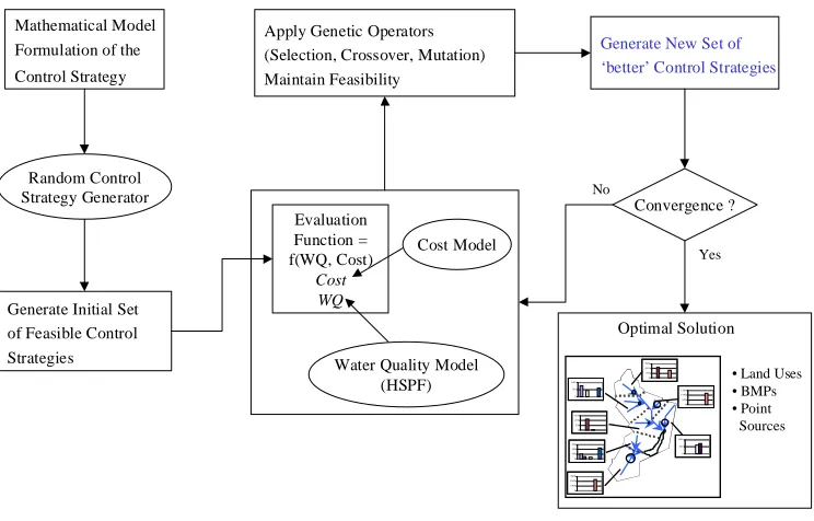
Figure 3.1 Genetic Algorithm-based Search Procedure... 51

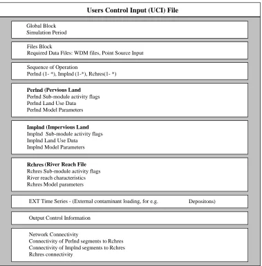
Figure 3.2 Users Control Input (UCI) ... 54

Figure 3.3 DSS Components and Interactions ... 57

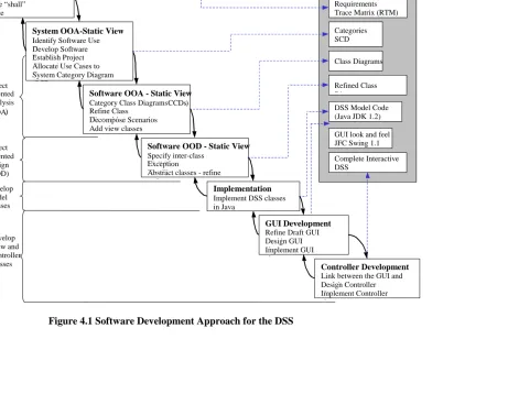
Figure 4.1 Software Development Approach for the DSS... 65

Figure 4.2 Sample Scenario ... 72

Figure 4.3 System Category Diagram ... 74

Figure 4.4 Interaction diagram for UC # 40... 75

Figure 4.5 Class diagram 1 for the categoryWQ_Management... 79

Figure 4.6 Class Diagram 2 for the categoryWQ_Management... 80

Figure 4.7 Class Diagram 1 for the categoryPS_Management... 81

Figure 4.8 Class Diagram 2 for the categoryPS_Management... 82

Figure 4.9 Class Diagram 3 for the categoryPS_Management... 83

Figure 4.10 Class Diagram for the categoryNPS_Management... 84

Figure 4.11 Class Diagram for the categoryLandUse_Planning... 85

Figure 4.12 Class Diagram for the categoryWQ_Model... 86

Figure 4.14 Class Diagram for child categoryGeneticAlgorithm of

Optimization_Algorithm... 88

Figure 4.15 Class Diagram for the child categoryLU of GeneticAlgorithm... 89

Figure 4.16 Class Diagram for the child CategoryPS of GeneticAlgorithm... 90

Figure 4.17 Class Diagram for the categoryUncertainty... 91

Figure 4.18 Class Diagram for the categoryView... 92

List of Tables

Table 2.1 Results for Unconstrained Optimization... 29

Table 2.2 Results for Constrained Optimization... 31

Table 4.1 Requirements Trace Matrix (RTM) ... 67

1

Overview

Environmental management problems associated with water quality in watersheds are inherently complex and are difficult to analyze due to many interactions among governing physical, chemical and biological processes and the impacts they undergo as a result of anthropogenic activities. Further, finding good management alternatives becomes exceedingly difficult due to conflicting issues such as cost, environmental impact and equity that need simultaneous consideration. Solutions to these problems require an integrated approach to the modeling, analysis and management of the watershed system.

The Better Assessment Science Integrating Point and Nonpoint Sources (BASINS) software system, (USEPA 1998) integrates a geographic information system, national watershed data, and state-of-the-art environmental assessment and modeling tools under a single platform. Within the current scope of BASINS, a user can employ existing computational utilities to develop alternative total maximum daily load (TMDL) strategies to achieve desired water quality targets. Although efficient, the BASINS system supports, at best, a trial-and -error approach to determining feasible TMDLs. This is still limiting given the large number of variables that a user can change and the needs for considering targets on numerous water quality parameters and multiple management criteria. The number of feasible combinations is very large, which makes a trail-and-error search process inefficient. A systematic search process is therefore recommended.

the DSS, the user may further modify these alternative strategies by trail-and-error to explore and examine more alternatives. Using these capabilities collectively, the user may engage in iterative search to efficiently identify “good” alternatives. The ambient watershed water quality is simulated by using water quality models supported within BASINS. The current implementation uses the Hydrologic Simulation Program – FORTRAN (HSPF) that is embedded within BASINS.

The DSS enables users to formulate various point source control strategies such as command-and-control (CAC), effluent charges and transferable discharge permit (TDP) programs, and non-point source control strategies such as land use planning, riparian buffer zoning, and system-wide detention ponds. An explicit quantitative analysis of the uncertainty to estimate the reliability of achieving the water quality targets is also supported within the DSS. The DSS also facilitates the propagation of the uncertainty in model parameters by using various stochastic sampling procedures such as Monte Carlo and Latin Hypercube sampling.

The mathematical models including the HSPF-based water quality modeling that represent the governing processes associated with watershed water quality are typically non-continuous and nonlinear. Therefore, the management optimization models that integrate these non-linear models are inherently nonlinear. As solving these management models using conventional optimization procedures such as linear programming (LP) and non-linear programming (NLP) solvers are not viable, a heuristic search procedure based on genetic algorithms (GAs) is employed.

the domain classes of the DSS with the user interface components. The Unified Modeling Language (UML) is used for the design. The implementation is carried out using the JavaTM platform (JDK1.2 and JFC 1.1).

A major component of this thesis research is the development of GA object classes and optimization model classes for use in solving optimization problems. A graphical user interface allows users to formulate non-linear, unconstrained as well as constrained optimization problems and solve them using a GA procedure. This set of GA object and user interface classes together comprise the Generic Genetic Algorithm-Based Optimizer (GeGAOpt). This tool improves upon existing general purpose GA tools and software by:

• allowing multiple decision variable representations;

• building optimization model structure that allows users to define the objective function and the constraints as functions of the decision variables;

• allowing for the use of various penalty function approaches for solving constrained optimization problems; and

• enabling users to access and run the GeGAOpt over the internet

2

A Generic Genetic Algorithm-Based Optimizer

2.1

Introduction

Genetic algorithms (GAs) are adaptive, global search procedures that are designed to mimic the underlying processes governing natural selection and evolution. A GA works on a population of individuals to identify relatively better individuals among the population, and combines the information embedded in the individuals to form newer

individuals that are generally better. Each individual represents a solution to an

optimization problem and the fitness of the solution is evaluated based on the performance of that solution in solving the given optimization problem. Through repeated application of a set of basic GA operators, including selection, mutation, and crossover, on the population of the individuals, the population generally converges to a solution that performs well with respect to the evaluation criterion. Although GAs do not guarantee global optima, in practice a population based search is robust as compared to local search approaches, and has been demonstrated to be quite successful in finding good solutions in an efficient manner. The following figure briefly illustrates a simple steady state GA procedure.

Optimization Model Formulation

Population: Set of Individuals

New Population

Convergence ?

No

Yes Generate Initial

Population

Optimal Solution Evaluate

Population Create Mating Population

by Selection Apply Genetic Operators

(Crossover, Mutation)

Figure 2.1 A Simple Genetic Algorithm

formulate generic mathematical optimization problems and solve them using a GA approach.

Various class libraries that include tools for using GAs to solve optimization problems have been designed. Wall (1995) developed the “GALib – A C++ Library of Genetic Algorithm Components” that enables users to perform optimization in C++ programs using several representations and genetic operators. The “GA Optimization Toolbox for Matlab” developed by Houck et al. (1995) implements simulated evolution in the Matlab environment using both binary and real representations and offers flexibility in choosing genetic operators, selection schemes and termination criteria. A user of these tools, however, should be knowledgeable of the various GA representations and operators, and sufficiently knowledgeable about the specific programming environment. To model problems that require multiple decision variable representations, the core modules of these tools need to be extended and built upon. For example, a mixed integer non-linear programming problem may require real and binary decision variables and the real decision variables may need to be represented by either real or binary numbers. For these mixed representations, the crossover and mutation operators need to be customized. The solution of complex constrained optimization problems using GAs requires these tools be supplemented with a complex fitness evaluation module that considers the relative significance of the constraint violations and their contribution to the fitness function. This requires the evaluation function to be hard coded for each problem.

The approach discussed in this paper results in the development of the tool Generic Genetic Algorithm Based Optimizer (GeGAOpt) that improves upon earlier GA tools by:

• supporting multiple representations within a single problem;

• obviating the need to re-code conventional genetic operators for complex problems that require multiple representations;

• enabling all of the above tasks with minimal user knowledge of the programming environment or of the coding of the GA operators; and

• enabling users to access remotely and run the GeGAOpt over the internet. The objectives of this research are to:

• develop GA object classes and classes that represent a generic optimization model for generic use;

• implement a graphical user interface that enables users to formulate generic mathematical function optimization problems and solve them by selecting from a combination of various decision variable representations, GA operators, and various approaches for handling constraint violations;

• demonstrate the use of the above interface for solving standard unconstrained and constrained optimization problems; and,

• assist users in understanding and exploring the working of GAs and in learning about GAs.

2.2

Organization

Section 2.3 discusses the software design and development approach adopted for the development of the GeGAOpt. Section 2.4 describes the development of the core GA modules, i.e., the data structures, representations, GA operators, etc. Section 2.5 describes an optimization model structure that allows users to define generic mathematical optimization problems and the use of various penalty function approaches for solving constrained optimization problems. The software design of the GeGAOpt is discussed in Section 2.6. Section 2.7 describes the features of the user interface of GeGAOpt. Section 2.8 discusses the solution of examples of non-linear and constrained function optimization problems that are solved using the various representations, operators, and penalty function formulations supported within the GeGAOpt.

2.3

Object Oriented Modeling and Design

understanding of requirements, cleaner designs and maintainable systems. OO technology is a way of thinking abstractedly about a problem using real world concepts, rather than computer concepts. The primary themes underlying OO technology are discussed briefly below:

• Abstraction consists of focusing on the inherent aspects of an object and

functionality. This avoids design and implementation decisions being made before the problem is understood.

• Encapsulation consists of separating the external aspects of an object that are

accessible to other objects from the internal aspects of the object. This prevents small changes in object structure from having massive ripple effects that affect the entire class hierarchy.

• Inheritance of the data structure and behavior allows common structure to be shared

among various classes. Inheritance is implemented using abstract classes and

interfaces. These are used as templates for creating subclasses.

The development of the GeGAOpt is based on these OO paradigm and design principles.

2.3.1 The Object Model

The object model captures the static structure of a system by showing its objects, the identity of and interrelationships among the objects. An object is defined as a concept or an abstraction. It captures concepts from the real world that are important to the application. A class is a static abstraction of a set of real world entities that have the same characteristics and share the same behavior. The principal features of a class are its

attributes, operations and its relationship to other classes. An attribute is a data value held by objects in a class. An operation is any function that may be performed by objects.

Classes are arranged into hierarchies sharing common structure and behavior.

Aggregation Relationship

This is an association based on the ‘whole/part’ concept. There are two types of aggregation relationships:

• Aggregation is a relationship where the ‘whole’ class does not have to create its ‘part’

class, but refers to the ‘part’ classes by reference,

• Composition is a relationship where the ‘whole’ part is responsible for creating its

‘part’ classes directly. This indicates a tighter coupling between the ‘whole’ and ‘part’ classes than is indicated by aggregation with reference.

Inheritance Relationship

This is an association between classes that focuses on similarities and dissimilarities among the classes with respect to their attributes and methods. An inheritance relationship exists between a superclass and a subclass. A subclass is a class derived from its superclass and inherits all the attributes and methods of its parent superclass. Association Relationship

An association relationship defines the nature of the coupling between two classes. In

this relationship, the interacting parts are visible to each other and may be shared between different aggregation hierarchies.

2.3.2 Object Model Representation

The object model is represented graphically with diagrams containing classes.

Classes are arranged into hierarchies sharing common structure and behavior. A package

is a collection of classes that are logically related. A class diagram describes the types of objects in the system and the various kinds of static relationships that exist among them.

Class diagrams also show the attributes and operations of a class.

2.3.3 Visual Modeling – The Unified Modeling Language

• a ready-to-use, expressive visual modeling language that can be used to develop and exchange meaningful models;

• extensibility and specialization mechanisms to extend the core concepts;

• a system representation that is independent of particular programming languages and development processes; and

• a formal basis for understanding the modeling language.

2.4

GeGAOpt Design and Implementation

This section discusses the conceptualization, the design, development and implementation of a set of object classes to represent the data structures and operators used in GeGAOpt.

2.4.1 Data Structure

Designing appropriate data structures to represent the hierarchy of genetic information content is of central importance to the GA search procedure. It is also essential to keep the design modular and sufficiently abstract so that it facilitates flexibility for further development.

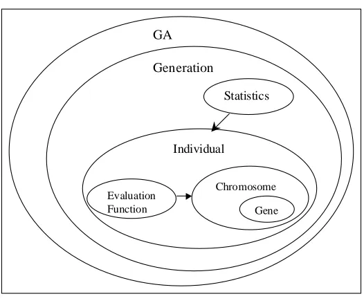
Typically, the hierarchy can be represented adequately by a gene at the lowest level. A chromosome is a vector of similar types of genes. An individual is a container for a set of chromosomes. The information necessary for evaluation of the fitness properties is encapsulated within the individual. A population comprises of a set of individuals and is the basic evolving unit. Individuals in a population undergo crossover and mutation to produce the next generation of individuals. Figure 2.2 depicts the composition of the various GA classes. The ovals represent the classes and the nested structure reflects the

Statistics

Chromosome Gene Evaluation

Function

GA

Generation

Individual

Figure 2.2 Composition of GA classes

The links represent the association relationships between the classes. A unidirectional link, i.e. an arrow, indicates that the association relationship is one sided. In this case, Chromosome ‘is visible’ to Evaluation Function.

2.4.2 Decision Variable Representations

The representation of a potential solution by an individual is the manner in which the genetic material is coded. Defining an appropriate representation is part of the art of using GAs. The representation should be minimal but completely expressive. The user should select a representation so that short, low-order schemata are relevant to the underlying problem and relatively unrelated to schemata over other fixed positions (Goldberg 1989).

The current GeGAOpt implementation supports real (r) and binary (b) representations for decision variables. A set of real decision variables can be represented either as a real string, as a set of binary strings, or a combination of both. Integer programming problems can be formulated by specifying the real decision variable to be of type r(0) or of type b(0) where the number in the parentheses indicates the number of decimal digits desired.

coded by the user by writing a class that implements the interface Operators. The primary operations implemented are crossWith(), mutate() and getDecisionVariableValue(). The user must select the crossover and mutation operators so that the integrity of the chromosome is preserved. For example, in a problem that depends on a sequence of items that lends itself to an order-based representation, crossover must generate reordered lists without duplicating any element in the list.

2.4.3 Selection Schemes

The selection operator ensures that the GA yields incrementally better individuals

in each generation. The individuals with larger fitness values get higher probability of being selected for mating than individuals having low fitness values. The selected

individuals are then placed in a mating pool. Individuals from this mating pool then

undergo crossover. The following selection schemes are supported: Roulette Wheel

In this type of selection, the probability of an individual being selected and placed in the mating subset is proportional to its relative fitness.

size population N

i individual of

fitness f

where f f P

i

N

i i i select

= =

=

∑

=1

(2.1)

This ensures that individuals with higher fitness have a better representation in the mating subset.

Binary Tournament Selection with Replacement

Two individuals are drawn at random from the population and the individual with the

2.4.4 Crossover Operators

The crossover operator defines the procedure for generating child individual(s) by mating two parent individuals. A crossover probability determines if the parent

individuals will cross to produce child individuals and the level of mixing of genetic

information. Convergence is rapid with higher crossover probabilities and may lead to premature convergence. The ideal crossover probability is problem dependent.

Individuals may consist of multiple chromosomes, in which case the corresponding

chromosomes of the two parent individuals P1 and P2 undergo crossover. Figure 2.3

illustrates the crossover procedure.

Procedure ‘Crossover’

1. Select two parent individuals, P1 and P2, for crossover.

2. if(Crossover) then

Do (P1 [Chromosomei] X P2 [Chromosomei])∀ i=1,Nc

where Nc is the number of chromosomes in an individual

3. else

Place P1 and P2 in the next generation.

Figure 2.3 Crossover Procedure

In the current implementation, the following crossover operators are supported. Single Point Crossover

For chromosomes ct_g = g₁,...,g_n and ct_h = h₁,...,h_n , a position k∈

(

)

randomly. The resulting child chromosomes are t _{k k n}

g g g h h

c 1,..., , 1,...,

1

+

+ _{= and}

n k

k t

h h h g g

c+1 = ₁,..., , ₊₁,..., .

Multi Point Crossover

For chromosomes ct_g = g₁,...,g_n and ct_h = h₁,...,h_n , a set of positions

)

(

{k k n

Uniform Crossover

For chromosomes n

t

g g g

c = 1,..., and n

t

h h h

c = 1,..., , a binary template

1 , 0 | ,...,

1 =

= t tn ti

T is generated randomly. The child chromosomes ct_g+1 andc_ht+1are

constructed as follows:

if(ti = 0) then

1

+

∈ t g

i c

g and h_i∈c_ht+1(no gene crossover)

else ∈ t+1

g

i c

h and ∈ t+1

h

i c

g (the parent genes gi and hi are interchanged)

Uniform Crossover with Recombination

This operator is similar to the uniform crossover except that the genes gi and hi are

combined to generate the child genes i i t

i fg f h

g +1 = +(1− ) and i i

t

i f g fh

h+1 =(1− ) + .

The fraction f is chosen randomly. A recombination rate controls the probability of recombination.

User defined crossover

The user may extend the abstract class Chromosome to implement specific crossover operators. Figure 2.4 illustrates an example of this.

class MyChromosome extends Chromosome { …

public Object[] conventionalCross { …user fills in code…

} }

Figure 2.4 User-Defined Crossover

2.4.5 Mutation Operators

The mutation operator defines the procedure for mutating each chromosome. Mutation introduces new genetic material into the gene pool of the population of

individuals. This may result in the exploration of previously unexplored points in the

increases population diversity. The ideal mutation rate depends on the characteristics of the decision and objective spaces. Hessner and Manner (1991) suggest that a good

estimate of the mutation probability is

) (

1

L

M , where M is the population size and L is

the length of the chromosome.

Mutation is different for different data types. For example, a typical mutation for a binary gene is flipping the bit with a given probability. In the current GeGAOpt, the following mutation operators are supported.

Random change mutation

This operator changes the value of a randomly chosen set of genes. The number of genes in this set can be specified by the user. For example, for a real number gene, this operator will randomly set the value of this real number to be a number between the minimum and maximum bounds of that real number gene. This mutation operator is suitable for

chromosomes of real number genes and genes having more complex data structures.

Swap mutation

This consists of randomly selecting two distinct locations within the chromosome and swapping the genes between the selected locations. This mutation is suitable for

chromosomes of binary genes and chromosomes where the permutation of genes needs to

be preserved, but is not applicable to complicated chromosomal data structures where the types of genes at different locations are different.

User Specific Mutation

The user can specify mutation operators in either of the ways shown in Figure 2.5.

class MyGene implements Operators { …

public void userSpecificMutate { …user fills in code… }

}

class MyChromosome extends Chromosome { …

public void userSpecificMutate { …user fills in code… }

}

Figure 2.5 User Defined Mutation

Elitism

supports generational elitism in which the worst individual in a generation is replaced with the best individual from the previous generation.

Figure 2.6 shows the different types of operators discussed above.

Elitism

No Elitism Generational Elitism Crossover

SinglePoint

Uniform MultiPoint

Uniform w/ ReCombination User Defined

Roulette Wheel SelectionScheme

Binary Tournament User Defined Swap

Mutation

User Defined Random Change

Binary Representation

User Defined Real Number

Figure 2.6 Operators and Representations supported in the current implementation

of GeGAOpt

2.5

A Flexible Framework for Optimization Model Formulation

2.5.1 Optimization Model Structure

A typical mathematical programming problem consists of the definitions of the decision variables, the objective function, and a set of constraints. The constraints and the objective function are expressed as mathematical expressions written in terms of the decision variables.

In the framework presented here, the mathematical programming problem is represented by a dynamic set of data structures. A set of classes is developed that emulates the conceptual framework of a mathematical programming problem. Using this set of classes, an instance of a user’s definition of the optimization problem can be constructed. This instance can then be solved to yield a solution to the optimization problem.

user’s definition of an optimization problem is then translated by a problem translator to an internal system representation of the optimization problem.

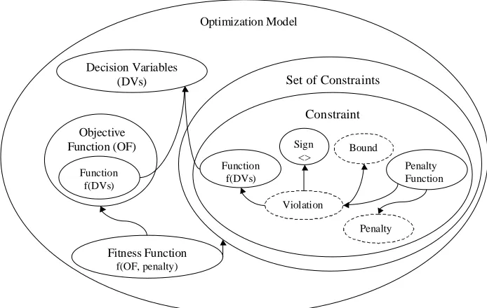
Figure 2.7 shows the composition among the classes that collectively represent the optimization model. In the following discussion, the Courier New font is used for the name of a class. The name of a class that represents an entity or object is placed in parentheses, immediately following the entity or object.

The optimization model consists of the decision variables, the objective function, the set of constraints, and the fitness function. The objective function consists of a function (Function). A constraint (Constraint) is composed of the classes, Function, Sign, PenaltyFunction and an instance of Bound. The dashed ovals indicate that Bound, Violation and Penalty are instances of the same class. The arrows indicate the uni-directional associations that imply that one class in the participating association is visible to the other.

Objective Function (OF)

Decision Variables (DVs)

Optimization Model

Fitness Function f(OF, penalty)

Function f(DVs)

Sign

<> Bound

Penalty Function Constraint

Violation

Penalty Set of Constraints

Function f(DVs)

Figure 2.7 Optimization Model Structure

space search feasible F function objective f variables decision of vector X where F X to subject X f MAX N N R R = = = ∈ : : ) ( (2.2)

The feasible search space N

R

F is defined by the constraints that are represented as:

s constraint of number total m s constraint inequality of number q i constraint for bound the rhs functions constraint h g where m q j X h q i rhs X g i j i j i i = = = = + = ∀ = = ∀ ≤ , , 1 0 ) ( , 1 ) ( (2.3)

The objective function f and the constraint functions gI and hj can be expressed in terms

of any combinations of standard functions of the decision variables. Without loss of generality, the optimization model described above considers maximization problems only. Minimization of the objective function f is achieved by maximizing the function -f.

2.5.2 A Framework for Solving Constrained Optimization Problems

It is difficult to develop a generalized constraint handling method that maintains the feasibility of solutions in a GA. Many approaches have been proposed for handling solutions that violate one or more constraints. Some of these approaches are described below:

2.5.2.1 Eliminating infeasible solutions

In this approach, infeasible individuals are eliminated from the population. It has been shown by Michalewicz (1995) that this approach is not effective for problems

having a small ratio (

N N N R R R S S F ∩

) of the feasible search space to the entire decision space

N

R

S . Eliminating good individuals that slightly violate some constraints, but are not too

2.5.2.2 Repair operators for infeasible solutions

New genetic material is introduced into the population by the crossover and mutation operators. The GA can be seeded initially with feasible individuals and the feasibility is maintained by application of repair operators. The design of this approach, however, is problem specific and involves having knowledge about a particular set of genes that causes the infeasibility. In complex problems, it may be difficult to check for all possible sets of genes for infeasibilities. The repair operators may add a significant computational burden to the GA, or they may distort some of the superior parent genes. In many cases, the problem of finding a feasible solution is itself NP-hard. The user should consider these shortcomings while designing the repair operators. The current GeGAOpt framework provides the user the flexibility to code specific repair operators such that feasibility is maintained, or use penalty functions to penalize the constraint violations.

2.5.2.3 Penalty Function Approach

Most methods proposed for handling constraints in GAs handle infeasible solutions by penalizing individuals for constraint violation. The constrained optimization problem is converted to an unconstrained problem by including the penalty explicitly in the objective function. This modified objective function becomes the fitness function for the GA. The modified fitness function is written as:

m i i constrait for function penalty p penalties constraint of function f function objective f function fitness F where X p X p X p f X f F X F i p m i p , 1 , )]) ( ),..., ( ),..., ( [ ), ( ( ) ( 1 = ∀ = = = = = (2.4)

The penalty for constraint i, pi, is zero for no constraint violation and is negative

otherwise. The functions F and fp are based on the users’ judgement of the relative

Linear Penalty Function

The penalty varies linearly with constraint violation and varies linearly with the generation number.

Exponential Penalty Function

The penalty varies exponentially with constraint violation and varies linearly with the generation number.

These penalty functions along with the function fp can be used to formulate fitness

functions used in most penalty approaches, notably those reported by Homaifar (1994), Joines and Houck (1994), Michalewicz and Attia (1994) and Harrell and Ranjithan (1999). The users can define the optimization problem and then experiment with various penalty functions and their associated parameters.

Figure 2.8 Linear and Exponential Penalty Functions

A problem that has equality constraints cannot be optimized easily for by GAs using the penalty approach. Even the slightest deviation from feasibility can cause an oscillatory behavior. In such cases, specifying a tolerance for constraint violation is known to result in stable convergence and improved performance. The constraint

violation tolerance δcvcan be specified for the constraints that are particularly hard to

satisfy. The penalty for constraint i is then calculated as:

otherwise

) (

if 0

X p penalty

Violation penalty

i i

cv i

=

≤

= δ

(2.5)

It is difficult to find an ideal combination of the penalty functions, pi, and the

combination is highly problem specific and depends on the response surface of the actual problem domain. The penalties obtained by using the above penalty functions are not dynamic, i.e., they are not varied based on observed population characteristics. A number of adaptive penalty methods that use the population characteristics for scaling the penalties based on the severity of the constraints have been proposed in the GA literature; e.g. Siedlecki and Sklansky (1989) and Smith et al. (1996).

The difference in the fitness values of the best feasible solution and the best infeasible solution is a measure of the severity of the constraints. This measure can be used to adaptively adjust the contribution of the constraint penalties to the fitness function as follows:

solution feasible

best the of value fitness F

solution best

the of value objective f

where

X p X p X p f F f X f X F

bf b

m i

p bf b

= =

− +

= ( ) ( ) [ ( ),..., ( ),..., ( )] )

( ₁

(2.6)

In this formulation, the best feasible solution yet found is comparable to infeasible solutions that have higher fitness values. As the sum of the penalties is weighted by the term (fb – Fbf), this term adjusts the magnitude of the imposed penalty during the progress

of the GA search. This approach is adequate for representing various adaptive penalty formulations including the one by Smith et al. (1996). This procedure is included in the current implementation of the GeGAOpt.

2.5.3 A Flexible Optimization Model Representation

A graphical user interface (GUI) is developed to provide the user the capability of formulating the optimization model in an algebraic textual format that is similar to the one used by conventional solvers. To provide this capability, an “intelligent problem convertor” is developed that converts a users’ mathematical definition of the problem to an internal problem representation that is based on the data structure shown in Figure 2.9.

Users Definition of Optimization Model

Intelligent Problem Converter

Internal optimization model representation

Providing the flexibility for users to define an optimization problem that consists of user defined decision variables and functions requires the use of an intelligent function parser that calculates the values of the user defined functions. The development of a function parser or interpreter is not a difficult task, but this results in considerable performance loss due to the fact the Java is an interpreted language itself.

To provide users the flexibility of defining a generic function optimization problem and to reduce the time associated with the evaluation, a Java Expressions Library (JEL), developed by Metlov (1998) is used. JEL enables the evaluation of the user-defined functions. JEL compiles mathematical expressions directly to Java byte-codes, allowing their fast evaluation. JEL supports all the Java primitive types as well as object types. Functions in JEL are methods of the Java objects. It does not require any front-end development for the functions. It is possible to use Java objects directly, exporting their functions to JEL. The integration of the optimization model with classes

in JEL, the GA classes, and the linkage with the user interface are described in the next section.

2.6

Design Features

The design of the GeGAOpt is based on UML methodology. The implementation of this system is carried out using the JavaTM platform. The Java programming environment provides a portable, interpreted, high-performance, simple, object-oriented programming language. This makes the design and implementation of the system simple, highly modular and promotes code reusability.

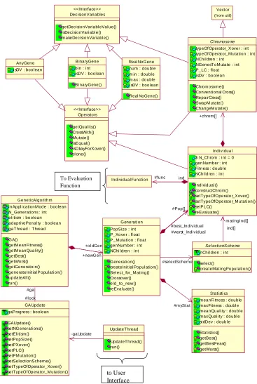
Figure 2.10 shows the GA classes and the inter-relationships among them. This figure is an UML class diagram that represents the conceptual GA structure discussed in Section 2.4.1. The gene classes as well as the classChromosome implement the interface

DecisionVariables. This facilitates the construction and evaluation of mathematical functions of objects that implement this interface. The class GAUpdate facilitates the synchronization of update threads (UpdateThread) spawned from the user interface seeking to update the GA operators and parameters.

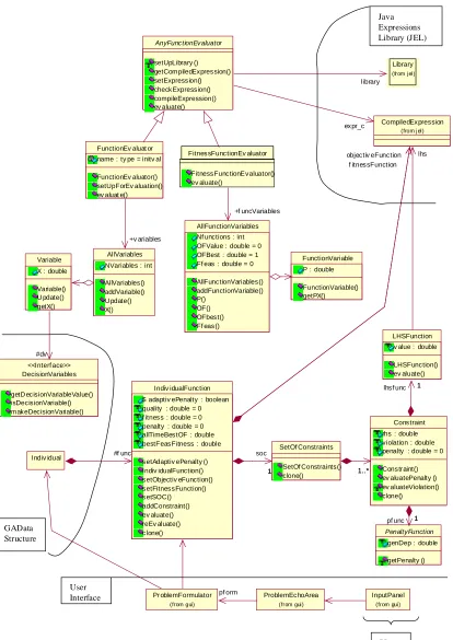
discussed in Section 2.5.1. The class IndividualFunction represents the optimization model and is responsible for the evaluation of the objective and fitness values. The arcs indicate the linkages between these classes and the GA data structure classes, the Java Expressions Library (JEL), and the user interface classes. The class

FunctionEvaluator facilitates the evaluation of user-defined mathematical functions of the decision variables. The class FitnessFunctionEvaluator enables the evaluation of the fitness function that is a function of the objective function and individual constraint penalties. The user interface classes InputPanel and ProblemEchoArea are responsible for enabling users to input and visualize any function optimization problem. The class ProblemFormulator converts the users’ definition of the optimization problem to an internal optimization problem representation. In this context, it represents the ‘intelligent problem converter’ in Figure 2.9.

Operators getQuality() CrossWith() Mutate() isE qual() isOkayForX over() cl one() <<Interface>> B inaryGene bi n : i nt isDV : boolean

B inaryGene()

Real NoGene num : double m in : double m ax : double i sDV : boolean

Real NoGene() DecisionVariables getDecisionVariableValue() isDecisionVari able() makeDecisionVari able() <<Interface>> AnyGene isDV : boolean

Vect or (f rom util)

UpdateThread

UpdateThread() run() GA Update

gaP rogress : boolean

GAUpdate() setNGenerati ons() setEli tism() setPopSize() setPXover() setPLC() setPM utation() setSelectionScheme() setTypeOfOperator_Xover() setTypeOfOperator_M utation() -gaUpdate

S tat isti cs meanFi tness : double maxFitness : double meanQuality : double maxQual ity : doubl e st dDev : double

Stati stics() getBest() getBestFeas() getWorst() GeneticAlgorithm

inAppli cationMode : boolean N_Generations : int el itism : boolean adaptivePenalty : boolean gaThread : Thread

GA() getMeanFitness() getMeanQuality() getBest() getWorst() getGeneratoin() generateInit ialP opulation() updateAll()

run()

#l ock #ga

IndividualFunction

Sel ecti onS cheme

nChil dren : int

select()

creat eMati ngPopulation() Generati on

PopSize : int P_Xover : fl oat P _Mutation : float genNum ber : i nt NChi ldren : int

Generati on() createIni tialPopul ation() Select_for_Mating() Crossover() old_to_new() reEvaluate()

#m ySt at +ol dGen

+newGen

#selectScheme

Chromosome

typeOf Operator_X over : int typeOf Operat or_Mutation : i nt NChildren : int

NGenesT oM utate : int P_LC : float isDV : boolean

Chrom osom e() Conventi onal Cross() RepairCross() SwapM utate() ChangeM utate()

Indivi dual $ N_Chrom : int = 0 genNumber : int Fitness : doubl e NChildren : int

Indi vidual () constructChrom () setTypeOfOperator_X over() setTypeOfOperator_M utation() setP LC() reEvaluate() ind #func ind[] m at ingInd[] #Pop[]

#best_Individual #worst _Indi vidual

+chrom []

To Evaluation Function

to User Interface

Library

(from jel)

FitnessFunctionEv aluator

FitnessFunctionEvaluator() ev aluate()

AllFunctionVariables Nf unctions : int OFValue : double = 0 OFBest : double = 1 Ff eas : double = 0

AllFunctionVariables() addFunctionVariable() P() OF() OFbest() Ff eas() +f uncVariables FunctionVariable P : double

FunctionVariable() getPX() DecisionVariables getD ecisionVariableValue() isDecisionVariable() makeDecisionVariable() <<Interf ace>> Variable X : double

Variable() U pdate() getX()

#dv

AllVariables NVariables : int

AllVariables() addVariable() U pdate() X()

FunctionEv aluat or name : ty pe = initv al

FunctionEv aluator() setUpForEv aluation() ev aluat e()

+v ariables AnyFunctionEvaluator setUpLibrary () getCompiledExpression() setExpression() checkExpression() compileExpression() ev aluate() library PenaltyFunction

genDep : double

getPenalty () InputPanel (from gui) SetOf Constraints SetOf Constraints() clone() ProblemEchoArea (from gui) Indiv idualFunction $ adaptiv ePenalty : boolean quality : double = 0 f itness : double = 0 penalty : double = 0 allTimeBestOF : double bestFeasFitness : double

setAdaptiv ePenalty () Indiv idualFunction() setObjectiv eFunction() setFitnessFunction() setSOC() addConstraint() ev aluate() reEv aluate() clone() 1 soc Indiv idual #f unc

Pr oblemFormulator

(from gui)

pf orm

Constraint rhs : double violation : double penalty : double = 0

Constraint() ev aluatePenalty () ev aluateViolation() clone() 1..* 1 pf unc LHSFunction v alue : double

LHSFunction() ev aluate() 1 lhsf unc CompiledExpression (from jel) expr_c objectiv eFunction f itnessFunction lhs 1 1..* 1 1 GAData Structure User Interface User Java Expressions Library (JEL)

2.7

GUI features – Interactive problem solving

2.7.1 Problem Formulation

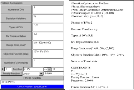
The user can formulate a function optimization problem through the problem formulation interface by specifying decision variables, an objective function, constraints, and a fitness function. The problem formulation panel is shown on the left in Figure 2.12.

//Function Optimization Problem //Saved file: omagosh.prb

//Non-Linear Constrained Optimization Demo //Decision Space R(0,100) x R(0,100) //Solution: at (x, y) = (17, 0)

Number of DVs: 2 Decision Variables: x,y Types of DVs: R,R DV Representation: B,B

Range '(min, max)': x(0,100);y(0,100) Objective Function (Max): 10*x + 6*y - 2*x*y Number of Constraints: 1

CONSTRAINTS #: 1

x + 2*y <= 17

Penalty Function: Linear Parameters: 2.0,0.0

Fitness Function: OF + 0.1*P(1)

Figure 2.12 Problem Formulation Panel and Sample Input File

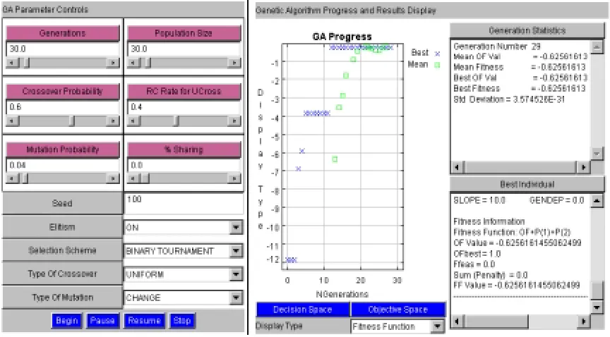
2.7.2 Controlling the GA Run

The user can dynamically control the GA parameters and operators listed below. • Crossover Probability

• Mutation Probability • Rate of recombination • Type of crossover • Type of mutation • Selection scheme • Elitism

• Population Size

• Number of Generations

• Seed for the random number generator.

Any combination of these parameters can be changed by the user at any point during the course of the GA run. The changed parameters take effect in subsequent generations. Based on the number of generations, the number of iterations that the GA population is allowed to evolve, the GA thread is suspended when this number is reached. The user can then either increase the number of generations to continue the GA run, or stop the GA run. The values for these parameters can be set by the user via the control panel which is shown on the left in Figure 2.13.

2.7.3 Monitoring Progress

The user can follow the progress of the GA run by monitoring the following:

• Fitness function, objective function and penalty function(s) values. A dynamic

display plots the convergence of the GA. The penalty values for the constraints can also be viewed.

• Decision space that depicts the values of the decision variables in the current

population (supported only for a two-variable problem).

• Objective space that depicts the values of the objective and fitness functions of

• Generation Statistics. The best as well as the mean fitness and objective function values of individuals and the standard deviation of the fitnesses of individuals in a population can be viewed on another dynamic display.

• The best solution. The characteristics of the best solution, i.e., the decision variable values, the constraint violations, penalties, objective function and fitness values can be monitored.

A display of these outputs is shown on the right in Figure 2.13.

Figure 2.13 Control Panel and the Results Display

2.8

Test Problems and Results

2.8.1 Unconstrained Optimization Problems

Table 2.1 shows the results of a series of GA runs for unconstrained function minimization problems. It reports the best, mean, and the worst solution found over a series of five independent runs that were carried out with different random number seeds.

The solution over a run is the individual that has the best objective function value. A

29

Table 2.1 Results for Unconstrained Optimization

# Problem Problem Description Bounds on Decision Variables

Known Solution Objective Function Value 1 DeJong F1

(DeJong, 1975)

∑

= 3 1 2 i i x Min 1,2,3 i 5.12 5.12 -= ∀ ≤

≤xi Min = 0

(x1,x2,x3) = (0,0,0)

best medium worst 0 -6.67E-6 -2E-5 2 DeJong F2

(DeJong, 1975) 2 1 2 2 2

1 ) (1 )

(

100 x x x

Min − + −

2 , 1 048 . 2 048 . 2 = ∀ ≤ ≤ − i

xi Min = 0

(x1,x2,) = (1,1)

best medium worst 0 0 0 3 Rosenbrock’s Function (Mathworks, 1997) 2 1 2 1

2 ) (1 )

(

100 x x x

Min − + − Min = 0

) 1 , 1 ( ) , (x1 x2 =

best medium worst 0 0 0 4 Goldstein-Price Function

(Goldstein and Price, 1971) )] 27 36 48 12 32 18 ( ) 3 2 ( 30 [ )]. 3 6 14 3 14 19 ( ) 1 ( 1 [ 2 2 2 1 2 2 1 1 2 2 1 2 2 2 1 2 2 1 1 2 2 1 x x x x x x x x x x x x x x x x Min + − + + − − + + + − + − + + + 2 , 1 2 2 = ∀ ≤ ≤ − i

xi Min = 3

(x1,x2) = (0,-1)

best medium worst 3 3.001947 3.0057

5 Test UF1

(Michalewicz, 1996) )} 20 sin( . ) 4 sin( . 5 . 21 { 2 2 1 1 x x x x Max π π + + − 8 . 5 1 . 4 1 . 12 3 2 1 ≤ ≤ ≤ ≤ − x

x Min = 38.85

(x1,x2) = (11.626, 5.725)

best medium worst 38.85 38.182 37.127 6 Test UF2

(Mathworks, 1997) (4 2 4 1 2 2 2 1)

2 2 2 1

1 _x + _x + _{x x} + _x +

e

Min x Min = 0

) 1 , 5 . 0 ( ) ,

(x1 x2 = −

2.8.2 Constrained Optimization Problems

Table 2.2 reports the results of a series of GA runs for constrained function optimization problems. It reports the best, mean and the worst solution found over a series of five independent runs that were carried out with different random number seeds. The solution over a runis the individual that has the best objective function value and is feasible with respect to all the constraints. A population size of 50 was used for problems TestCF1 through TestCF4. The crossover probability was varied from 0.5-0.7 and the number of generations required for convergence varied from 50-100.

A population size of 60-70, a generation number of 300-400, crossover probability of 0.4 and a mutation probability of 0.04 were used for problems TestCF5,

TestCF6 and TestCF6. The value

N N N

R R R f

S S F

r = ∩ , which indicates the ratio of the feasible

search space to the total search space, reported by Michalewicz (1995) for these problems are also shown in this table. The low rf values indicate that these are highly constrained

problems. Due to the highly constrained nature, the performance of the GA search is sensitive to the penalty functions and fitness formulations used in solving these problems. A suitable set of the penalty functions was identified through a trial-and-error process and then five independent runs were carried out with different random number seeds.

31

Table 2.2 Results for Constrained Optimization

# Problem Problem Description Bounds on Decision Variables

Known Solution Objective Function Value 1 Test CF1

17 2 . 2 6 10 : ≤ + − + y x st xy y x

Max Max = 170

(x1,x2) = (17,0)

best medium worst 170 169.62 169.12 2 Test CF2

(Mathworks, 1997) 10 0 5 1 : ) 1 2 4 2 4 ( : 2 1 2 1 2 1 2 2 1 2 2 2 1 1 <= − ≤ + + + + x x - x - x x + x . st x x x x x e

Min x _{Min = 0.0236}

(x1,x2,) = (- 9.5474, 1.0474)

best medium worst 0.0236 0.0258 0.0296

3 Test CF3

(Mathworks, 1997) #2 0 , 0 2 1 ≥ ≥ x

x Min = 8.5

(x1,x2) = (0,1.5)

best medium worst 8.5 8.5 8.5 4 Test CF4

(Floudas and

Pardolas,. 1997) 2 2 0

) 7

12

4+ − =

− x y

st.

*y + y*y *x -

Min (- Min = -16.7389

(x, y) = (0.71751,1.470)

Best medium worst -16.739 -16.728 -16.703 5 Test CF5

(Michalewicz, 1995) 0 2 0 2 0 2 3 , 2 , 1 0 8 10 ) ( 2 10 ) ( 2 10 ) ( 2 . ) ) ( 5 : 12 9 8 11 7 6 10 5 4 9 12 11 3 2 12 10 3 1 11 10 2 1 13 5 2 4 1 ≤ + − − ≤ + − − ≤ + − − = ∀ ≤ + − ≤ + + + ≤ + + + ≤ + + + − − + = =

∑

∑

i Min = -15

X =

(1,1,1,1,1,1,1,1,1,3,3,3,1)

Six constraints active at the global optimum all except,

3 , 2 , 1 0 8 + 9 ≤ ∀ =

− xi x+i i

Table 2.2 Continued

# Problem Problem Description Bounds on Decision Variables

Known Solution Objective Function Value 6 Test CF6

(Michalewicz, 1995) 0 11 5 2 3 4 0 8 6 23 196 0 10 3 7 282 0 5 4 3 2 127 . 8 10 4 7 10 ) 11 ( 3 ) 12 ( 5 ) 10 ( : 7 6 2 3 2 1 2 2 2 1 7 2 6 2 2 1 5 4 2 3 2 1 5 2 4 3 4 2 2 1 ) 7 6 7 6 4 7 2 6 6 5 2 4 4 3 2 2 2 1 ≥ + − − + − − ≥ + − − − ≥ + − − − − ≥ − − − − − − − − + + + − + + − + − x x x x x x x x x x x x x x x x x x x x x st x x x x x x x x x x x Min 7 ,..., 1 10 10 = ∀ ≤ ≤ − i

xi Min=680.63

X=

(2.3305, 1.9514, -0.4775, 4.3657, -0.6245, 1.0381, 1.5942)

The first and last

constraints are active at the global optimum. 3 121 . 5 − = ∩ E S S F N N N R R R best medium worst 681.34 684.93 688.8

7 Test CF7

(Michalewicz, 1995) 0 7 ) 8 ( 12 6 3 0 30 3 ) 4 ( 2 ) 8 ( 5 . 0 0 6 14 2 ) 2 ( 2 0 40 2 ) 6 ( 8 5 0 120 7 2 ) 3 ( 4 ) 2 ( 3 0 12 2 5 2 8 0 2 17 8 10 0 9 3 5 4 105 . 45 ) 7 ( ) 10 ( 2 ) 11 ( 7 5 ) 1 ( 2 ) 3 ( ) 5 ( 4 ) 10 ( 16 14 : 10 2 9 2 1 6 2 5 2 2 2 1 6 5 2 1 2 2 2 1 4 2 3 2 2 1 4 2 3 2 2 2 1 10 9 2 1 8 7 2 1 8 7 2 1 2 10 2 9 2 8 2 7 2 6 2 5 2 4 2 3 2 1 2 1 2 2 2 1 ≥ + − − − ≥ + + − − − − − ≥ + − + − − − ≥ + + − − − − ≥ + + − − − − − ≥ + + − − ≥ − + + − ≥ − + − − + − + − + − + + − + − + − + − + − − + + x x x x x x x x x x x x x x x x x x x x x x x x x x x x x x x x x x st x x x x x x x x x x x x x x Min 10 ,..., 1 , 10 10 = ≤ ≤ − i

x_i Min =24.306

X=

(2.172, 2.3639, 8.7739, 5.096, 0.9906, 1.4306, 1.3216, 9.8287, 8.2801, 8.376)

Six out of eight constraints are active at the global optimum

(all except the last two)

2.9

Conclusions and Recommendations

2.9.1 Conclusions

The GA object classes and the optimization model classes can easily be customized for application to a wide range of problems and be used in education and research. The GeGAOpt developed in this study facilitates the formulation of non-linear unconstrained as well as constrained optimization problems and their solution using the underlying GA framework. This makes it possible for a user familiar with mathematical programming to solve optimization problems using GAs and explore the effect of various representations, genetic operators, penalty functions, and static and adaptive penalty techniques on the GA search. The results discussed in Section 2.8 effectively demonstrate the use of the GeGAOpt in this solving various unconstrained as well as constrained optimization problems.

This framework has been developed based on OO paradigm and design methodology. This makes it easier for further development and enhancement of the current capabilities. The framework is generic in that, it can be easily extended to represent complex chromosomal data structures such as trees and networks.

The graphical user interface to this framework currently enables only the formulation of function optimization problems. The availability of the GeGAOpt via the internet enables users to explore the features of the GeGAOpt with the help of a Java compatible web browser.

2.9.2 Recommendations for Future Development

The current framework can be extended to support two as well as three-dimensional matrix representation of chromosomes and complex data structures such as

n- ary trees, graphs and networks. Genetic operators that are appropriate for these data

References

1. Booch, G., Rumbaugh, J. and Jacobsen, I., (1997). Unified Modeling Language for

Object-Oriented Development, V 1.1, Rational Software Corporation, Santa Clara,

CA.

2. De Jong, K.A., (1975). An Analysis of the Behavior of a Class of Genetic Adaptive

Systems, Doctoral dissertation, University of Michigan, Abstract International},

36(10), 5140B, (University Microfilms No 76-9381).

3. Floudas, C.A., and Pardalos, P.M., (1987). A Collection of Test Problems for

Constrained Global Optimization Algorithms, Springer-Verlag, Lecture Notes in

Computer Science, Vol.455.

4. Fowler, M. and Scott, K., (1997). UML Distilled: Applying the Standard Object

Modeling Language, Addison-Wesley.

5. Goldberg., D. E., (1989). Genetic Algorithms in Search, Optimization and Machine

Learning, Addison-Wesley.

6. Goldstein, A.A and Price, J.F., (1971). On descent from local minima. Mathematics of Computation, 25:569-574.

7. Gosling, J., Joy, B., Steele, G, (1989). The Java Language Specification, Addition-Wesley Publishing Co., Inc., Reading, MA.

8. Joines, J.A., and Houck, C.R., (1994). On the Use of Non-stationary Penalty

Functions to Solve Nonlinear Constrained Optimization Problems with GAs, in

Proceedings of the First IEEE Conference on Evolutionary Computation, pp. 579-584.

9. Harrell, L.J., Ranjithan, S.R., (1999). Evaluation of Alternative Penalty Function

Implementations in a Watershed Management Design Problem, Proceedings of the

Genetic and Evolutionary Computation Conference, July 13-17 at Orlando, FL, pp. 1551-1556.

10.Hessner, J.; Männer, R., (1991). in Proceedings of the First Workshop on Parallel Problem Solving from Nature (Lecture Notes in Computer Science, Vol. 496); P. Schwefel and R. Männer (Eds.); Springer-Verlag, Berlin, pp 23-31.

12.Homaifar., A., Lai, S.H., Qu, X., (1994). Constrained Optimization via Genetic

Algorithms, Simulation, Vol. 62, No. 4, pp. 242-254.

13.Houck, C. R., Joines, J.A. and Kay, M. G., (1995). A genetic algorithm for function optimization: A Matlab implementation . NCSU-IE Technical Report 95-09.

14.Mathworks, (1997). Matlab v. 5.3 Manual, URL: file:/afs/bp.ncsu.edu/dist/matlab53/help/fulldocset.html.

15.Metlov, C., 1998. Java Expressions Library (JEL) Reference Manual, URL: http://galaxy.fzu.cz/JEL.

16.Michalewicz, Z., (1996). Genetic Algorithms + Data Structures = Evolution

Programs, Springer-Verlag.

17.Michalewicz, Z., (1995). Genetic Algorithms, Numerical Optimization and

Constraints, Proceedings of the Sixth International Conference on Genetic

Algorithms, Morgan-Kaufman, pp.151-159.

18.Michalewicz, Z., and Attia, N., (1994). Evolutionary Optimization of Constrained

Problems, Proceedings of the 3rd Annual Conference on Evolutionary Programming,

World Scientific, pp. 98-108.

19.Object Management Group (1997). UML 1.1 Documentation. URL: http://www.rational.com/.

20.Siedlecki, W., and Sklansky, J., (1989). Constrained Genetic Optimization via

Dynamic Reward-Penalty Balancing and Its Use in Pattern Recognition, in

Proceedings of the Third International Conference on Genetic Algorithms, pp. 141-150.

21.Smith, A.E., Coit, D.W., and Tate, D.M., (1996). Adaptive Penalty Methods for

Genetic Optimization of Constrained Combinatorial Problems, INFORMS Journal on

Computing, Vol. 8, No. 2, pp. 173-182.

22.Tamiz, M. and Mardle, S.J., (1998). An interactive graphics-based linear, integer and

goal program modeling environment, Decision Support Systems, 23, pp. 285-296.