I. Hydrodynamic model selection for counter diffusing systems: A selectivity study in mass transfer with non-linear chemical kinetics. II. Effect of catalyst poisoning on selectivity: A modelless approach. III. Selectivity optimisation for complex non-lin

Scholarship at UWindsor

Scholarship at UWindsor

Electronic Theses and Dissertations Theses, Dissertations, and Major Papers

1968

I. Hydrodynamic model selection for counter diffusing systems: A

I. Hydrodynamic model selection for counter diffusing systems: A

selectivity study in mass transfer with non-linear chemical

selectivity study in mass transfer with non-linear chemical

kinetics. II. Effect of catalyst poisoning on selectivity: A modelless

kinetics. II. Effect of catalyst poisoning on selectivity: A modelless

approach. III. Selectivity optimisation for complex non-linear

approach. III. Selectivity optimisation for complex non-linear

reaction schemes. IV. Reactor simulation for the hydrogen fluoride

reaction schemes. IV. Reactor simulation for the hydrogen fluoride

reaction: Fluorspar + sulphuric acid products

reaction: Fluorspar + sulphuric acid products

R. Raman Sood

University of Windsor

Follow this and additional works at: https://scholar.uwindsor.ca/etd

Recommended Citation Recommended Citation

Sood, R. Raman, "I. Hydrodynamic model selection for counter diffusing systems: A selectivity study in mass transfer with non-linear chemical kinetics. II. Effect of catalyst poisoning on selectivity: A modelless approach. III. Selectivity optimisation for complex non-linear reaction schemes. IV. Reactor simulation for the hydrogen fluoride reaction: Fluorspar + sulphuric acid products" (1968). Electronic Theses and Dissertations. 8080.

https://scholar.uwindsor.ca/etd/8080

I HYDRODYNAMIC MODEL SELECTION FOR COUNTER DIFFUSING SYSTEMS--- A

SELECTIVITY STUDY IN MASS TRANSFER WITH NON-LINEAR CHEMICAL KINETICS. II EFFECT OF CATALYST POISONING ON

SELECTIVITY A MODELLESS APPROACH

III SELECTIVITY OPTIMISATION FOR COMPLEX NON-LINEAR REACTION

SCHEMES

IV REACTOR SIMULATION FOR THE HYDROGEN FLOURIDE REACTION--- FLOUR SPAR +

SULPHURIC ACID ►PRODUCTS.

A Thesis

Submitted to the Faculty of Graduate Studies Through the Department of Chemical Engineering in Partial Fulfilment

of the Requirements for the Degree of Doctor of Philosophy at the

University of Windsor

by

R. Raman Sood

Windsor, Ontario

1968

INFORMATION TO USERS

The quality of this reproduction is dependent upon the quality of the copy

submitted. Broken or indistinct print, colored or poor quality illustrations and

photographs, print bleed-through, substandard margins, and improper

alignment can adversely affect reproduction.

In the unlikely event that the author did not send a complete manuscript

and there are missing pages, these will be noted. Also, if unauthorized

copyright material had to be removed, a note will indicate the deletion.

®

UMI

Copyright 2008 by ProQuest LLC.

All rights reserved. This microform edition is protected against

unauthorized copying under Title 17, United States Code.

ProQuest LLC 789 E. Eisenhower Parkway

DEDICATED TO:

Leslie Dickirson my dear friend

/

ACKNOWLEDGMENTS

Academically, I owe a great deal to Dr. G.P.

Mathur. This is another occasion for the acknowledgment of that debt. During the period that this work was being

done, his sense of perspective was invaluable.

A large number of individuals have helped me

in my work; some even whose names I do not remember and others whom I know very well. I wish to thank Dr. M*

Bhatia, Dr. S. Srivastva and H. Toes, for helping me develop

a sense of quantified simplicity, and Dr, R. Stager for encouraging me to look at the problems from an outsider’s

point of view.

I want to take this opportunity to express my

gratitude to the staff of the computer centre for a

generous allotment of time, to D. Chambers and Mrs. E.

KcGaffey for help in the University Library, to R.K. Roongta

for help in the drawing work, and to my friends who put up with me during two years of a de-humanizing and alienating

nightmare.

The financial support from the National

Research Council of Canada in the form of Graduate

Fellowships is truly appreciated.

"Because of past studies chemical engineers are prone to accept, as a general rule the previous conclusion, that different theoretical models predict almost the same reaction effects on overall mass transfer rate... The selection of a correct model is indeed very important,.."

C.J. Huang and C.H. Kuo A.I.Ch.E.J. 11, 901

(1965) in a discussion on the effects of

diffusivities.

ABSTRACT

A two step non-linear complex reaction scheme 2M]--- ^2M2--- *~M3 has been used to establish the need for

a careful selection of a mass transfer model for counter

diffusing systems. By comparing the Penetration Theory and

Film Theory selectivity parameters, it is shown that the two fluid-mechanical models do not predict the same results.

It is also shown that the deviations between the results predicted by the two models do not appear to be directly

related to increasing complexity in the reaction kinectics.

In addition, the effect of reaction order on the selectivity parameter, has been examined by varying the order of the

second step reaction.

ii

ABSTRACT 11

TABLE OF CONTENTS 111

FIGURES v

TABLES vi

I. INTRODUCTION 1

II. REVIEW OF LITERATURE 4

III. THEORETICAL MODEL OF THE SYSTEM 8 IV. DIFFUSION EQUATION

A. General Diffusion Equation 10

B. Mathematical Statement of Penetration Theory 12 C. System Equations according to the Penetration

Theory 15

D. Solution of Penetration Model System Equation 20 E. Quantitative Aspects of the Film Theory 30 F. System Equations for Film Theory 31 G. Solution of Film Model System Equation 33

V. RESULTS 43

VI. DISCUSSION OF RESULTS 67

VII. CONCLUSIONS , 75

APPENDIX A 77

APPENDIX B 83

APPENDIX C . 8 5

APPENDIX D - .91

APPENDIX E 95

n o m e n c l a t u r e BIBLIOGRAPHY

iv

Figure

1.1 ' COMPARISON OF FILM AND PENETRATION MODELS FOR THE TWO STEP REACTION Ml— -M2— - M3 Ml— M2 1.0 ORDER, M2— -M3 1.0 ORDER.

1.2 COMPARISON OF FILM AND PENETRATION MODELS FOR THE TWO STEP REACTION Ml— -M2— -M3 Ml— —M2 1.0 ORDER, M2 -M3 1.5 ORDER.

1.3 COMPARISON OF FILM AND PENETRATION MODELS FOR THE TWO STEP REACTION Ml -M2— -M3 Ml— -M2 1.0 ORDER, M2— M3 2.0 ORDER.

TABLES

Tables

I— VIII °BAf/<rBAp

IX— XVI (BAf/<rBAp

XVI-XXIV BAf / °BAp

Tables for the case where the second step reaction is of 1.0

order **3-50

Tables for the case where the second step reaction is of 1.5

order 51-58

Tables for the case where the second step reaction of 2.0

order 59-66

vi

INTRODUCTION

The solution to the problem of predicting the

effect of a liquid phase chemical reaction on gas absorption

or vice versa, has been attempted by proposing a hydro-

dynamic model of the gas-liquid interface and the liquid flow pattern. Amongst the various models suggested, the so called film theory model‘postulated by Nernst (25),

Lewis and Whitman (24) and the penetration-surface renewal

theory model proposed by'Higbie (14), Kishineveskii (17) and

Danckwerts (9 ), are the two that are most commonly used.

When the diffusion coefficients of various reacting species are the same, the results predicted by the film theory and

LI

the laminar and turbulent boundry layer theories are found

to be in remarkable agreement with each other. This

interesting fact has been pointed out by Brian and

Beaverstock (4), Kishineveskii and Armash (18), Astarita

( 1 ), and a few others. Basing their conclusions on the

results available -in the literature, Brian et al ( 4) concluded, " This insensitivity to the fluid mechanical models used suggests that the theoratical predictions will be good approximations even for physical systems which

depart considerably from the idealised models." In a

2

the mass transfer model invoked has little influence on the

predicted ratio of the mass transfer coefficient with

chemical reaction to the physical mass transfer coefficient. Conclusions of this nature, have led in the past to

a rather indiscriminate selection of models for the prediction of the transfer coefficient ratio

[

fluid-fluid systems. It is to be noted that the conclusion

regarding the insensitivity of predicted results to the hydrodynamic model used, is of fundamental importance; but,

it has been arrived at on the basis of results obtained

from studies dealing with relatively simple systems in which,

the products of chemical reaction can never cross the phase boundary. The lone exception is the work of Szekely and

Bridgewater (31.) . On the basis of their investigations of

a linear kinetic system with a volatile intermediate, they questioned this alleged insensitivity of predicted results

to the model selected. It was decided therefore, to undertake a detailed study with a view to determine, whether or not, the predicted transfer coefficient ratio

is always insensitive to the hydrodynamic models used. In order to do so, it was proposed to compare the film and

penetration model selectivity of an intermediate, Ivl2, formed during a complex reaction described below:

kl 2M1 + [3] --- 2 M2

k 2

2M2 +[g] M3 _(ii)

(i)

(iii)

[ i r r ] = 2 k 2 [f° ' 2kl ^ 0

(iv)

The component Ml diffuses from a fluid 'a1

into another fluid 1 g* where it reacts to form an intermediate M2. It is further assumed that M2 can either react to form

M 3 or diffuse back into f l u i d ’a * . The stipulation that M2 can diffuse back across the interface makes this study

different from thi© ones conducted thus far. According to Bridgewater ( 5 ) systems of this type are encountered in the liquid phase oxidation of hydrocarbons by absorbed oxygen.

As mentioned before, the commonly used index for comparing

various hydrodynamic models is the transfer coefficient

ratio; but, in this case it was decided to use a n 'equivalent

CHAPTER II

REVIEW OF LITERATURE

Peaceman (27). in 1951. compared the film and penetration theory solutions for several kinds of chemical reactions and found that these solutions were in

close agreement with each other, as long as the diffusion coefficients of the various reacting species did not differ

significantly from each other. Similar results were reported

later by Danckwerts and Kennedy (11). The reactions treated

by these authors however, were one-step reactions. Brian and Beaverstock ( ^ ), analysed a two step reaction of the type:

A (gas) ^ .. A (liquid)

Liquid Phase:

A + C (already in liquid) ► B (nonvolatile)

B + C - ■ - ► D (nonvolatile),

and found that if the diffusion coefficients for various components were similar, the results from the penetration

theory and film theory would not differ significantly.

The components, 1B *,*C ' and 'D* were assumed to be

nonvolatile and thus could not cross the liquid-gas

phase boundary.

k

penetration - surface renewal theories, derived equations

for the ratio of interphase mass transfer accompanied by a first order reversible reaction. They found that when the

diffusivities of the reactants and the products are nearly

equal, the effect of chemical reaction on the overall mass transfer ratio is insensitive to the model adopted for calculations. Kishineveskii et al (18) and Astarita ( 1 )

reached similar conclusions from their analysis. It must be

emphasized again that in all these studies, the products of the chemical reaction could not cross the phase boundary.

Szekely and Bridgewater (31) investigated the

fluid - fluid system,

kn k2

A --- -— ► B --- ► C (1) dC

dr 1 A

dC ,

= k-p (2 )

= * 2 CB - k lCA (3) dr

in which, both A and B are volatile ( A diffuses from a fluid a into fluid 3, where it reacts to form B, which

in turn can either diffuse back into a or can get converted

to C ), Because the product of reaction fB ’ could cross the phase boundary, it was possible to compare the transfer

coefficient ratio for 'B' instead of- ’A'. Szekely et al (3D found that the selectivity of the intermediate B, as

6

models, differed by as much as 22%. .Th’e difference in the results obtained by Szekely et al (31) and Brian et al (4),

can be attributed to the different assumptions made in these

studies concerning the nature of the intermediate 'B'. Thus, whereas in Brian et al's ( ) investigation, 'B' could not cross the phase boundary, in Szekely et al's (31)

investigation, 'B' could diffuse through the fluid - fluid

phase boundary.

In reporting their results, Szekely et al (31) conjectured that other counter diffusing fluid - fluid

systems involving more complicated kinetics would display the effect of hydrodynamic patterns more severely. Since

the kinetic scheme they investigated involved only first order reactions, the resulting equations for both the film

theory model and the penetration models were linear and

hence quite easy to solve.

Useful as Szekely et al's (31) results are,

their conclusions have the following shortcomings:

i. Linear reactions are an exception rather than a rule in actual chemical engineering practice, and Szekely et al's

(31) conclusions are certainly not applicable to cases of nonlinear kinetics. They could only make conjectures

regarding the effects of " more complicated kinetics",

ii. Szekely et al (3D have investigated only one case and it can be thought of as an isolated example rather than

as a general conclusion.

It is obvious that in order to show the

relative importance of model selection for the prediction

of the transfer coefficient ratio in a counter diffusing heterogeneous fluid - fluid system, it is necessary to

undertake a much more extensive investigation. This study

was primarily undertaken with that purpose in mind. Its major objectives are listed below;

i. To establish the relative importance of model selection

for heterogeneous counter diffusing fluid - fluid : systems with nonlinear kinetics; that is, to

quantitatively establish the sensitivity of predicted

transfer coefficient ratio to the hydrodynamic model

used,

ii. To check Szekely et al's (31) conjectures about the effect of more complicated kinetics on the sensitivity

CHAPTER III

THEORETICAL MODEL OF THE SYSTEM

The system considered is one in which a fluid species Ml. present in a fluid medium 'a1, diffuses into a fluid »£•,

Ml( fluid a )- — ■ ^ mi ( fluid £ )

where it reacts with the fluid ’g 1,

2Ml + [p]---- ► 2M2 .

The fluid component M2 then either diffuses back into the

medium ’a 1 or undergoes another irreversible reaction :

2M2 + [g]--- ► M3 .

In this analysis Ml and M2 were treated as gases, whereas

(5 was assumed to be a liquid. However, this treatment is

equally valid for liquid - liquid systems. It was assumed that R was in such an excess that its concentration could be

considered constant. As Danckwerts (10) and Carberry (7 )

have shown, absorption into liquids can generally be regarded as an isothermal process. Physical and chemical properties of the system were assumed to be constant. It was also assumed that the diffusive fluxes of species Ml

and M2 did not interact. Some further simplifying

assumptions that were made in the course of this study are

listed below s

i. The diffusion coefficients of Ml and M2 are equal. This assumption is realistic in light of the fact that

8

depends only very slightly on the solute concentration, ii. There is no resistance to mass transfer in the gas phase.

Thus the concentration of species Ml at the gas liquid

interface, corresponds to the equilibrium partial

pressure of Ml in the bulk gas phase. This assumption does not in any way limit the scope of the problem.

The equilibrium assumption is also made for species M2 , iii. The back pressure of the species M2 in the gas phase

is zero. This assumption was made for the sake of

simplicity and standardisation,

iv. No appreciable change in volume takes place as a result

of the chemical reaction,

v. Fluxes of MU and M2 from the gas phase towards the

liquid phase are positive.

The assumptions listed above apply equally

well to gas liquid contacting, in packed towers, in wetted wall columns, and to gas absorption into stagnant liquids.

For the system under investigation,

selectivity was defined as the ratio of the rate of

formation of the intermediate M2, to the rate of depletion

of the reactant jvjq. Selectivity defined in this vray is

equivalent to the ratio of the surface flux of M2 to that of the surface flux of Ml. This definition has been used

CHAPTER IV

DIFFUSION EQUATION

A. General Diffusion Equation

For a reacting species i, the mass balance over a moving small element of liquid, near the gas liquid interface, is described by the partial differential

equation :

Molecular Transport = Convection + Accumulation

+ Reaction Rate.

The Lagrangian System of Coordinates is used for the derivation of this equation.

The diffusion equation as written above is of

very little practical value and is generally simplified by making one or more of the following assumptions t

i. D^ , the diffusivity is constant. This assumption is a good approximation except in the case of polymer

solutions, where D^ is strongly dependent on the concentration of various species,

ii. The velocity U is constant over the moving small element of the fluid under consideration.

Equation (4) can therefore be written as

(5) 10

. Each liquid element moves as a single whole with a

constant velocity, like a plug in a plug flow reactor.

It is implied that there is no motion in a direction perpendicular to the interface, or U=0. With U=0,

equation (5 ) is reduced to

Equation (6) is a mathematical statement of the penetration - surface renewal model.

. The concentration profile of a species i in the

element is independent of time. This assumption leads to the statement of the so-called film theory model.

Thus,

Equations (6 ) and (7) can he further simplified by assuming that the radius of curvature of the gas

liquid interface is very large in comparison to the

depth of the diffusion / penetration layer, and thus the diffusion process is one-dimensional. According to Levich (23), this condition is almost always fulfilled

in real cases. In Cartesian Coordinates, equations (6 ) and (7 ) can accordingly be written as

DiA ci = + r ₍₆₎

61

DiACi r ₍₇₎

B. Mathematical Statement of Penetration Theory

Equation (8 ) is a statement of mass balance over a small element of liquid in contact with the

interface. This equation has been derived under the

assumption of a zero velocity gradient in a direction

normal to the interface. If the chemical reaction term is dropped, equation (8 ) can be written as

If the element of liquid under consideration can be assumed to have :

i. the characteristics of a plug of an infinite depth

moving as a whole with a constant velocity, or can be treated as a stagnant element of infinite depth i.e.:

The d e r i v a t i o n of equation (12) is described in Appendix IA. 6Ci

6t •

(10)

0 < x < co (11a)

ii. a uniform initial concentration Ci :

Ci = C i ; t = 0 0 < x < oo

■ 0

(lib) Ci = Ci ; t > 0 X — >• oo

*

iii, an interfacial concentration Ci :

*

(llcc) Ci = Ci ; t > 0 x = 0

then, the flux X(t) at exposure time t and at the

interface can be expressed as

X(t) = - Di (12)

~ *

The average flux, X(t), for an exposure or penetration time of t* is given as

o (Dl^ l )x= 0 d t

X ( t )

I

(13)

where, K^p = 2

ilk)

\ TT t

J dt o

In accepted chemical engineering terminology ~/ o , * o .

X ( t # ) = KLp ( Ci - Ci ) (15)

(15a) T nt

Kj(p is the penetration theory liquid phase mass transfer coefficient without chemical reaction.

Equation (12) has been derived with the help of assumptions (11). These assumptions are very stringent

and are strictly true in rare cases only. Under the

conditions imposed by assumptions (11), equation (12) can

have only very limited applicability. Danckwerts (9 ) has listed the conditions under which equation (12) can be

applied as a close approximation to :

i. liquid layers of restricted depth, and

ii. liquid moving parallel to the surface with a velocity

14

The necessary condition for (i) is that the

time of exposure should be so short that the depth of

penetration is less than the depth of the liquid; for (ii), it must be so short that the depth of penetration is less

than the depth at which the velocity is appreciably

different from that at the surface. By the term depth of penetration is meant the distance from the interface over

o

which Ci is appreciably different from Ci. Danckwerts (9 )

has arbitrarily defined the penetration depth as the distance from the interface at which the rise in

concentration is 1/100 that at the surface.

Equation (12) has. been extensively used for

describing mass transfer for situations comparable to

conditions (i) and (ii). The resulting models are of great help in understanding the phenomena occuring in industrial equipment. Thus, Brian et al (3 )# have described the

phenomena of mass transfer in a packed absorption column by assuming that the liquid flows down over a piece of

absorber packing in slug laminar flow. Absorption is

thought to take place by unsteady molecular diffusion and

accumulation within a slug of liquid as it flows down the packing and is exposed to the gas phase for a given contact time interval. The liquid is assumed to be instantaneously

and completely mixed in flowing from one piece of packing

to the other, and to be free of velocity gradients and

transport process adjacent to the gas liquid interface.

Thus, each new contact time interval is begun in each slug with a flat concentration profile for all components. The

contact time between successive mixing points is so short that the absorbed species never penetrates deeply enough

to approach the wall of the piece of packing. Therefore, the liquid depth can be taken as infinite for the sake of mathematical simplicity. The descriptions for spray and

bubble absorbers as well as for wetted wall columns that

satisfy considerations (i) and/or (ii), have been given by

Higbie (14).

C. System Equations According to the Penetration Theory

1. Chemical Rate Equations :

Ml (gas) < Ml (liquid) (16)

Liquid Phase:

. kl

-(1?)

2 mi f a 2 M2

M2 (liquid)— i M2 (gas) (13)

Liquid Phase:

k2

(19)

2M2 + 0 M3

The rate equation for step (17) is,

If p is present in large excess, its concentration can

be assumed to be constant. Thus equations (20) and (21) can be written as

- ^ M l n

= 2 k ^ Cj q ( 2 2 )

d r

dC.jrx m u

' ~ & f = 2 M2 1 M1 (23)

2. Mass Balance Equations s

For the reacting system described by equations (16 - 23), the following mass balance can be written:

n 6 ^41 SCMi n ^

Ml

T T •

1

Ml

1

J

DM2 i f * * = ! ! k t Z ^ S z . k i C ^ ) (25)

6x^ 51

The appropriate initial and boundary conditions are

as follows :

t = 0 0 < x < 00 = 0 (26a)

t > 0 x = 0 CH1 = 4 ^ (26b) t > 0 x —*• 00 Cj^ —*. 0, bounded (26cc)

t = 0 0 < x < co q42 = 0 (27a)

t > 0 x . = 0 ~ 0 (2?b)

In equations (2^ - 27) 't* refers to the instantaneous time in the life of a liquid element. The boundary

conditions (26) and (27), are mathematical statements

of the underlying assumptions of the penetration theory.

Boundary conditions (26a, 27a) were chosen for

convenience only. Any other bulk concentration can be used. The boundary condition (27b) states that though 'M2’-can diffuse back into the gas, its concentration

at the interface is zero. This numerical value was chosen for convenience. It should be noted that this

boundary condition is different from the normally

The equations (2^ - 2?) were non-dlmensionalised to : 0 ¥9

assumed condition ( — — )x-0 = 0 ( which express the 6x

6C M2

nonvolatility of the species M2 ).

62a 6a

+ an (28)

6y2 60

(29)

e > o

e > o

0 = 0 0 < y < oc

y — oc a -► 0 bounded a = 1

a = 0 (30a)

(30b)

18

0 = 0 0 < y < oc b = 0

0 > 0 y = 0 b = 0

(31a) (31b) (31cc)

0 > 0 _{y -*} oc b -►0 bounded.

The transformations used to obtained these dimensionless equations are listed under the mass transfer section of

t

the nomenclature ( Page 1Q0 ).

3. Reaction Diffusion Modulus :

Equations (2^ - 2?) have to be solved with a view

to determining the average value of the expression

time. One index of this predetermined time that is

often used in mass transfer literature is the reaction diffusion modulus ^ derived by making a suitable

, over a predetermined period of

substitution for t in the expression for Ko

Lip

In this . is chosen. ( See the transformation used for non dimensionlising t ).

LMlp (33)

TT

where % = _{/ K?„LMlp}

The definition of selectivity iBAp' leads to

6c

<r

B A p ' =

Average of _

D ( — *-2 )

M 2 6x x=° Average of r f ^ Ml \

- l m i^ 57 “ x=o

over

predetermined value of the exposure time 't'.

<r

BAp

v f ^ “ 6CM2 //6x ^x=0 dt

o________________________

£

f ( - 6^ / S x )X=Q dt

In non dimensional terms 6

BAp = v Jk

i / ( - 6b/6y ) d0

f ( - 6a/6y ) de

o Y=0

For v - 1, equation (37) is some times written as,

a

BAp =

/ ( - 6b/6y )y=Qd9

y[n/kQ J ( - 6a/6y )y=0A'

In this form,

(34)

(35)

(36)

(37)

20

<r

BAi

Mass Transfer Coefficient with chemical reaction „

for M2 Mass Transfer Coefficient without chemical reaction

Mass Transfer Coefficient with chemical reaction

for MlJ Mass Transfer Coefficient without chemical reaction

(3?b)

D. Solution of Penetration Model System Equations

<r

In order to evaluate ABp (equation 37) for various values of 9 ( or corresponding values of ) ,

it is necessary to solve equations (28) and. (29) along

with the Initial and boundary conditions (30) and (31). Closed solutions for these equations, except for the case

m = n = 1 , are not known. For mathematical simplicity and because of limitation on computer time, only the

following cases were considered ;

1 . v - 1, m = 1 , n = 1

2 . v = 1 , m = 1 ,5 . n = 1 3 . 1/ = 1 , m = 2 , n = 1 .

Detailed description of the methods used in

solving these .special cases of equations (28) and (29), follow on the succeeding pages.

** n = 1 was chosen because of limitation on computer time. The numerical methods described on the following pages

apply equally well to cases where n ^ 1 .

1 . v =1 , m=l, n=l.

Equations (28) and (29), with initial and

boundary conditions (30) and (31), were solved with the help of the Laplace Transform Tables (28), the step by step

procedure is given in Appendix (IA). Szekely et al (31) erlve the final solution as

a = 1

f

(38)

(A)

yVT

e ,>VAerfc / y - VT 0 j + e erfc^ y +

e ^erfc /_y - VfT\ + e^erfc/ y + V I H V

and

(39)

e

/ /-6a\ d9 = ^ \

fiyyy=o-(4o)

CD

-0

/evT+ _ i \

\ 2VT/erf

22

BAp =

(i-x)

1-4 0 V T + 1 jerf (20

. 7T 2vry

•

/

i

2% (v»j V*-;

, 2 . v ,20V 2 0 /a0 + i\erf/ P\ + P

P [yfiT/ tt

. (k/n y

(42)

2 and 3* General Procedure for Numerical Solutions

For n=l, and */=l, equation (29) can be written as,

59 m

'b = 6b + Xb -1 6 Y 69

-y y \1

e erfc( y - + e erfc( y + ^ j j \2Ve

(43) An analytic solution of equation (43), is not known for when m / 1. However, numerical techniques employing finite

difference methods are available. Out of the two types of

finite difference schemes, explicit and implicit, an implicit

scheme was chosen. This was done because implicit schemes

2

are inherently stable for all values of A 9 / A y > 0

(see equation 1?C Appendix C). On the other hand explicit schemes are easier to operate, though they are time consuming

2

because of stability condition A 9 / A y <1/2 (see equation

13C Appendix C). The boundary condition (31C) is always a problem in numerical calculations as it involves the division

of a semi-infinite length into a finite number of mesh

divisions. As mentioned by Secor et al (29) this difficulty can be dealt with in several ways, A practical infinity can

be defined and the region 0 < y < oo practicai can be

divided into a uniform mesh. This approach results in a coarse grid in the region of interest (close to the

interface i.e. y = 0 ) and results in a corresponding lack

of accuracy. However, by using a non-uniform mesh (fine mesh in the region of rapid change and a coarse grid far

away from the surface), or a very fine mesh, this difficulty can be overcome. The latter method is time consuming; whereas

lack of precise knowledge about the location of the regions of rapid change makes the method of non-uniform grids unwork­ able .

The space "0 < y < oo , 0 < 6 " was there­

fore mapped onto a semi-infinite ( in 0 ) rectangle

”0 < z < 1 , 0 < 0", by the transformation

y = cz

1—z ( W .

Thus at y=0, z=0 and at y=oo, z=l. The constant, c is used

to distribute the grid according to the experimenter's needs.

A larger c means a finer grid near the interface and a coarser

grid at the other end of the space coordinate. A proper value -of c can be selected only after experimentation. A value of

c = 0.98 was chosen, after comparing the analytical and numerical results for the case of m = 1 .

24

m 6 /6b dz \ 6b + Xb -1 6 ^ 6 - dy' = § 9 2

-cz/(l-z) .

e erfc / cz _vo (t u

cz 1-z + e erfc

z)2vo- )

+ VeT" / cz + V&i \TlTzT2Vf /

6Jb dz = 6_b (1-z) 5z dy §z c

(45)

(46)

2

6 /6b dz \ = 6 dz (6b dz\ = 6^'b /dz\ + 6b dz 6 Idz\ fiyVfiz dy/ 6^ dy \62 dy/. 5z2 \d3y $z dy 6"z \dy/

Equation (47) leads to,

(Z{ 1-z) \

6ZV c2

)

? 2 4 3

6 b = 6 b (1-z) _--- - 6b/2 (l-z) ‘ 6y oz c

(47)

(48)

With these transformations, equation (43) is changed to,

m 3 2 4

6b = a - Xb - 26b (1-z) + 6 b (1-z) (49) 69

where,

a = 1

2

iz c2

Oz C

-cz,/(l-z)

erfc( cz - v r

z)2Vd

)

+ e

cz/(l-z)

erfc ^ cz + Ve“

(i-z)2va

)

with the boundary and the initial conditions:

9 > 0

6 = 0

z = 0 b=0

0 > z > 1 b=0

(50a) (50b)

9 > 0 z — ► 1 b = 0 (5Occ) The implicit finite difference approximation for the equation

(49) can he written as,

m

b b a lb

i. .1+1 - i, .1 = i,j+l - i» j A 0

-b b \ . 3

1*3+1/ " l+l,

j+1__-A Z

(1 - Az(i-l) )'

„2

b 2b b

+ I i+1,3+1 - i, .1+1+ 1-1, .1+1 A Z

where,

(l-(i-l) A z ) , ,

i=l,2,..,N-1

3=1,2, , ,M-1 (51a)

a

1*3+1 V ( l - ( i - l ) A z ' y T ^

c( (i-l)Az)/(l-(i-l)Az)

erfc / c( ic( i-1 )Az + i/jA9 l)Az ) 2.fT^Q

i=2,3, .. . N-l

3=1,2,...M-l

(51b).

26

The equations (50a, 50b, 50cc), in the form useful for digital computations, are:

b ^ ^ j j = 0,0 j = 1,2,.., M (52a )

b(i = 0.0 i = 1,2,... N (52b)

k(N,j) = ^ = ^ (52cc)

where,

M = A0 + 1 (53)

0

N = _1 + 1 (54)

Az

The following values of A 9 a n d A z were used:

0 < 0.02 A 6 = 0.0001

6 > 0.02 A 6 = 0.018

Az = 0.02

Equation (51a) can be written as,

r 3

b i+l,j+l 1 2(1-( 1-1 )a z) A9 - (l-(i-l)Az) A 0

[ A z ° 2 a z 2c2

J

. _ ... . 3. . ^

+ b , . .V ri-2(l-(i-l)AZ)A0 + 2(l-(i-l)Az) A9 1 i,j+l --- — ---

2-2---L A Z c A Z C

J

= AQa. . _ - A0Xb“ . + b. . 1,0+1 i,0 i,j

i = 2,3,... N-l

j = 1,2,3,... M-i (55)

Equation (55) has the following triangular form,

SB2pb2,j+l + SC2pb3,j+l = SD2p

SA3pb2,j+l + SB3pb 3,j+l + SC3pb4,j+i = sD3p

SA^pb 3, j+1 + W \ j +i + Sc^Pb5,j+l = SD3p

!AN-2pbN-3, 3+1 + SBN-2pbN-2, i+1 + SCN-2pbN-l, j+1 “ SDN-2

SAN-lpbN_2, j+1 + SBN-lpbN-l,J+l“ SDN-lp

(56)

w h e r e ,

sA l p =

A z c

i = 3,4,;.. N-l (57a)

3-n. = 1 ■2(l-(i-l)Az)"Ae +' 2(l-(i-l)Az) A0

jjlp x--- p---

p-p---2 2 2

A Z c A Z c

i = 2,3,...N-l (57b)

3 - 4

_ 2 (1- ( i-1 )a z ) A9 - (l-(i-l)Az) A9

U J-P — p 9 9

28 N-2 (5?cc) N-l M-l (57d) Equations (56), and hence, (55), can be solved by Gaussian elimination to obtain the values of b on the line j + 1

(for details of the method, see Appendix D).

Douglas (12) has shown that the round-off error for this numerical method is less than the discretisation

error for the usual choice of A z and A0 . It is to m

be noted that the term, (X b ) was evaluated on the line •j1 instead of 1 j + 1*. This was suggested by Lees (22),

who showed that equally accurate results can be obtained m

if terms such as, (b ), are evaluated on the line 1j1

instead of the line ’j + l 1. This modification of the

usual implicit finite difference scheme, however, results

in a linear triangular system of equations, instead of m

- the non linear ones that would result if (b ) was

evaluated on the line ’ j + l 1, Lees (22) has indicated that there vrould be a five to six fold reduction in machine tine as a consequence of this modification. As an

/ m

experimental check, the results for (b .), were compared

i * .1 i = 2 ,3 * * •«

SCN-lp “ 0

m

S = A9a - A0Xb. . + b. .

Dip i ,j+1 i.J i,j

i = 2,3,... j = 1 ,2 ,.,, and m = 1 .5 ,2 ...

improvement was found, and all further calculations, were ' m

therefore done for (bi j). As a test of convergence for the solution, calculations were repeated, with half the

normal values of time and space increments. The improvemen

was found to be less than 1 fa. In order to calculate ?r

BAp according to equation (3?)» the values of the term

e

6b\ d 0 and / (- d 0 are needed.

by)y=o o \ fly/y=°

0

f (- ^a i 80 » was by using equation (^4-0), whereas

JQ \ 6y/y=o

0

6b\ d 0 , was evaluated as follows 6y/ y=o

0 / 2 \ 0

f6 /_ 6b\ d© = f (_ 6b\ f-(l-z) ) d© = l / / 6b\

s ^ fiy/y=0 o \ fiz/ \ O / z=0 c o ^ $z/z=0

(58) The integration for (58), was done by Simpson’s rule.

(see Appendix A).

Knowing,

6 <r

f

L

J ^ i y ) y = o J0 V by )y= o

various values of m,\, and ^ (or the corresponding 0). The P

results are tabulated in Tables (1-2/0.

30

E. Quantitative Aspects of the Film Theory:

The Nernst (25), Lewis and Whitman (2^) film

theory, although earlier in its origin, can be treated as a

special case of Higbie’s (l^) penetration theory, if it is assumed that the small element of liquid referred to in

Higbie’s model attains its final concentration profile instantaneously. This amounts to a stagnant film of

thickness, b^ , next to the gas liquid interface. A similar film can be visualised on the gas side of the interface.

The other assumptions of Higbie’s theory are retained. In

the context of the film theory, the assumptions made can be

stated ass

. . i. Outside the two films, the concentration of reactants in the bulk of the two phases is uniform.

ii. The velocity profile in the film is flat. This

corresponds to the penetration theory assumption of zero velocity gradient in a direction normal to the interface.

Stagnant liquids and liquids moving under laminar flow

conditions approximate this situation closely.

iii. The resistence to mass transfer is totally within the film, wherein molecular transport takes place by Pick’s law.

If the term ’r ' is neglected in the equation (9)> the resulting equation can be written as

D, d C 1 = 0 dx2

= C^ ; X=0

; X =

/ d C \ D /•» o \ o /* o \

X ■ X = (- V ) , 0 = i p - ^ i0 ^ ) « ° > ’

where, §Lf = D ^ f (6l)

is the liquid side mass transfer coefficient without

chemical reaction.

F. System Equations for Film Theory:

- Equations (16-23) which describe the chemical processes occuring in the gas liquid system are valid for the film theory as well. The mass balance equations for the film theory are however different. These will now be

enumerated:

1. Mass Balance Equations According to the Film Theory

For a reacting species i

2

d C n . . .

Mi— = l Ml (62)

dx

2

d C _{m n}

% 2 ---= 2k C 2k c • dx2

32

The boundary conditions chosen are

*

x = 0 CM1 = CM1 (64a)

x = *f CM1 = 0 (64b)

x = 0 CM2 = 0 (65a)

x = ^ cM2 = ° (65b)

x > ^ a - b = 0 (65cc) Boundary conditions (65a) is a suitable boundary condition

for a volatile substance. The value (x = 0 = 0) for (65a) was chosen for convenience. These boundary

conditons match the boundary conditions for the penetration

model. Equations (62-65) can be non dimensionalised to

2 2 n

d a _ </> a (66)

, 2 ^

dy

2 2 m 2 n

d b i / A ^ b V & a (67) . 2 “ f " f

dy

y = 0 a = 1 (68a)

y = 1 a = 0 (68b)

y = 0 b = 0 (69a)

y = 1 b = 0 (69b)

The selectivity £ according to film theory is defined as i5A

dC -D M2

M2

----O' r] y

BAf = ax

x=0

(70)

- DMldCMl dx In non-dimensional form,

x=0

BAf = 1 (-db/dy) y=0 (71)

v (-da/dy) y=0

For if = 1, equation (71) can also be written as

<r

BAf

(

(

Like the penetration model equations, equationss (66- 69) can be solved analytically only for the special /

case of i = n = 1, Solutions for cases corresponding to (a, b, c) of the penetration theory were attempted.

1 , v = 1 , m - n - 1

The solution of equations (66, 68a,b) is,

( i l f - \ b y\ / \ ^ C o s h ^

a = Sinh I f 1 ) , (da\ f f

3^

b =

' ' tanh 3inh (73)

,-D dC .

_ M2__M2 / \

BAf = J dx I = \-db/dy/y=Q "DMldCMl /-da/dy \y=0

✓3 T T \ /

3x

aBAf = - / 1 Vl- VjT tanh#f

tanh 0 VT -- f

(7*0.

2, and 3• Numerical Solutions for

v — l,n = 1 , m = 1 .5 * 2.0

Like it's counterpart in the penetration equation,

equation (67) when written as,

2 m 2

2 b - \p Sinh ib -\b y

d b = f _f_____ f f (75),

, 2 Sinh \Jj

f

has not been solved analytically for the boundary conditions

(69a and 69b) unless m = 1. As equation (75), (69a and 69b)

pose a two point non linear boundary value problem j they cannot be solved by any of the usual numerical techniques involving superposition of two solutions. The

Quasilineurisation technique due to Bellman ( 2 ) and

Kalaba (l6 ) was selected. This technique coupled with the

✓

fourth order Runge-Kutta integration method has been used

by Lee (20) for the solution of the axial diffusion model

iT = 1 was adopted to save computer t i m e . Quasilinearisation * can take care of any n/ 1 .

0.3 ) for optimisation and control problems. Instead of

directly solving the non linear differential equation, the

solution, when it exists, is obtained as a limit of a

sequence of functions representing solutions of linear

differential equations. Quasilinearisation provides a technique for the construction of this monotone sequence

of functions which converge to the solution of the non linear equation. This representation is achieved by the

use of the ’maximum operation’ . The linear differential equations, whose solutions constitute the elements of the

monotone sequence, can be easily solved with the help of

the principle of superposition. The progress towards convergence is quadratic in the sense that each iteration

doubles the number of digits of accuracy. The method is

briefly outlined in the Appendix (XC) and its application

to equation (75) is given in the following pages. .a, Quasillnearisation

The right hand side of equation (75) is a continuous function of b and y for all y € D (0 < y < 1 ).

It is twice differentiable with respect to b over the

domain of interest and has a bounded second partial

derivative with respect to b. It is also clear that this expression is a strictly convex function of b over the

36

solution of equation (75) can be obtained as the least

upperbound of the sequence generated by the recursion

relations

l M - x* f ( V 7,) B '

L ° J \ / Sinh ^

+ ^bQ (y ) - vQ (y)^ (y)j (76)

where,

l [ ] = V [ ]

L J dy2 <??>

2

r . r\ ,2 m - \l> SinhU - j)

L |b, (y)| = 0.Xb (y) - f V'f /+

L 1 J f 0 — nTTvny;---Sinh^>

^ ( y ) - bQ (y)\ ^ '|b” _1 (y)^ (78)

and,

r t 2 m 2 / \

L [bn+l(y^j = ^fXbn(y ) " ^ S i n h ^ f-^fyJ Sinh \b

*f

+

(bn+l <y) -

Vy

)

)

(

1

(

y

)

)

El = 1.5, 2 (79)

The boundary conditions for both (7 6 ) and (78) are

bn ( 0 ) = ° bn ( l j = °

n - 0 , l,,,,n

vo ( 0 ) = ° vo (1) = 0 (80)

Equation (76) and (79)1 with boundary conditions (80)

are second order linear differential equations with

variable coefficients. In order to start the generation of the sequence, all that is heeded is a guess at the

function v (y) . From a knowledege of the physical situation, and for the purpose of computational

convenience, v (y) was assumed to be

0 = vQ (y)j 0 < y< 1 (81) With the assumption stated in equation (81), equation

(76) can be solved analytically to give

bo (y);0<y < 1. Two methods the fourth order

Runge-Kutta technique and the finite difference formulations

are available for the solution of equation (78) and similar equations that follow. Since b (y) is found

analytically it is possible to store values of

bQ (y),0 < y < l , in the computer memory, but the same is

not true for b^(y). Values of b^(y) can be calculated and stored at discrete intervals of A y only. If the Runge-Kutta integration procedure is adopted for the evaluation of

b2 (y), the step size has to be increased to 2 Ay, as the values of b^(y) at points halfway between b^(y) and

"b^(y + A y ) are required. Thus, if no interpolation polynomial is used, each iteration doubles the step size

for a Runge-Kutta integration method. Therefore, without

interpolation in five iterations, an eighty division mesh

gross errors. Other stability problems commonly associated

with marching integration techniques also reduce the

efficacy of the Runge-Kutta method. During computations for this problem, for example, it was found that for

X > 0 . 1 , the Runge-Kutta technique yielded unstable results for m = 1.5 and 2. Despite these difficulties

encountered in the use of the Runge-Kutta method, the

marching technique has been used by Bellman ( 2),

Kalaba (1 6 ), and Lee (20).

Sylvester et al (30) were the first to use the finite difference scheme in conjunction with

quasilinearisation. Lee (21) has recently solved his old axial diffusion model tubular reactor problem using the

finite difference method. The finite difference formulation being less accurate than the Runge-Kutta techniques, it

(the finite difference scheme) must use a smaller step size for integration. This in turn results in the use of

more computer time. Equations (76-80) can be described

in the finite difference form as follows:

A y2

,\p Sinh ^ - ^ ( i ~ l ) Ayj

S i n h ^

( b 0(i) - ',„ ( i ) ) ( m l ^ o ( S ) '

i = 2,3,... N-l (82)

bo ( i r ° 5 bo(N)=0 and N= ~Ay + 1 (82a)

Equation (82) can also be written as

(

A y ^ S i n h ^ (i- 1)av ^

Sinh^

1=2,3,... N-l (83),

l(i-l) “ l(i) + l(i+1) _ x J hm

--- ^ ~ X ^fbo(i)

Ay

^ S i n h V^( i-l)Ay^

('

Sinh^

2 m-1 ’K l ) “bo(i)j^ ^ *fb° 0 ) ' ■

ko

51 o r bl(N)= bo(l)= bo(N)= 0 (8^a)

and, b

n-HO-l) n-fl(l) n+l(n-l) _ ^2\ b ^ .j-0 Sinh 0„(i-l)Ayj

A y 2 f n i 1--- /

Sinh 0 f

+ (bn+l(l)-bn d ) ) 4 \ T i ) t

i=2,3,... N-l (85)

bn+l(l)=bn + l ( N r bn(l)=bn(N)=0 (85a)

Equation (85) can also be written as

/ 2 2 m-1 \

b - ( 2+ Ay mX 0■ b , . . lb , 4 +b , n+l(i-1) V ^f n(i)/ n+1(1) n+l(i+l;

(l-m)^Ay2 0 \ b“ (i)j- A y 202sinh | 0 f- ^ ( i - l ) Ayj ,

Sinh "0

i = 2,3,... N-l (86)

Equations (83, 84, and 86), along with the boundary conditions (82a, 84a, and 85a), represent a triangular system of

equations of the form:

SB 2 f b n(2) + SC2fbn(3) = SD2f

SA3fbn(2) + SB3fbn(3) + SC3fbn(4) = SD3f

SA^fbn (3) + SB4fbn(4) + Sc4fbn(5) = sD4f

SA(^-2)fbn(N-3) + SB(M-2)fbn(N-2) + SC(N-2)fbn(N-l)“ SD(N-2)f

SA(N-l)fbn(N-2) + SB(N-l)f.bn(N-l) = SD(M_l)f (87) with,

SA . = 1, i = 3,4,... n-l (88)

/ 2 2 m-1 \

SBif = ~(2 + A y mX^ bn(i)) ’ 1 = 2 «3.... N-l (89) Sc ,f = 1 , i = 2,3,... N-2 (90)

(

- ' s Sinh $

i= 2,3,... N-l (91) These equations can be solved by Gaussian elimination (see

Appendix D ) . In calculating the concentration profile of ' b', the interval 0 < y < 1 was divided into two-hundred

2

parts. For X < 10 , with seven iterations (n = 6), five

2 4

digit accuracy could be obtained. For 10 < X < 10 , in order to obtain the same accuracy, ten iterations were

needed. Experiments were made with A y = .0025, but no

improvement in accuracy could be made. Knowing (da/^y)y = 0 f

calculated for various values of m,\ and ip. The results

are presented in tables (1-2*0,

RESULTS

TABLE I

Reaction Ml *~M2 is of 1.0 order and M2 ► M3 is also of

1.0 order.

^ (the reaction diffusion modulus) = 0.100000E+00

$ (the time)=

X

0.100000E-05

0.100000E-03 0.100000E-01

0.100000E+03

0.100000E+05

0.127272E-01

FILM MODEL

- % k f

-0.331990E-02

-0.327012E-02 -0.331848E-02 -0.3H793E-02

-O.896769E-O3

PENETRATION MODEL

a

BAp -0.421910E-02 -0.421902E-02 -0.^21919E-02

-0.376804E-02.

- 0 .899782E-03

RATIO

aBAf/?Ap

0.786873E+00 0.775091B+00

0.786521E+00 0 .827467E+00

2ji|

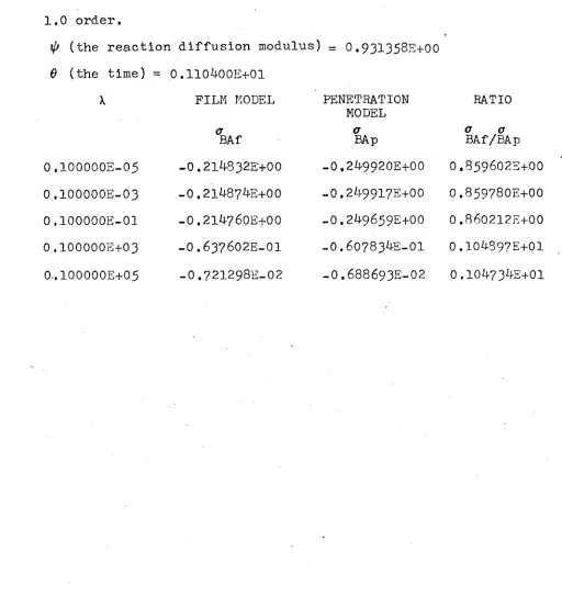
TABLE II

M2 is of 1.0 order and M2 *-M3 is also of

reaction diffusion modulus) - O.931358E+OO Reaction Ml

1.0 order.

ip (the

6 (the time) =

\ 0 .100000E-05 0 .100000E-03 0 .100000E-01 0 .100000E+03 0..100000E+05 0.110400E+01 FILM MODEL a BAf -0.21^832E'+00 -0.21^-87^E+00 -0.21^760E+00 -0.637602E-01 -0 .721298E-02 PENETRATION MODEL a BAp -0.2i|-9920E+00 -0.2^9917E+00 _o.2^9659E-}-oo -0 ,60783^-E-oi -0 .688693E-02 RATIO

a a

BAf/BAp 0.859602E+00 O.85978OE+OO 0.860212E+00 0.104897E+01 0 .10^73^2+01

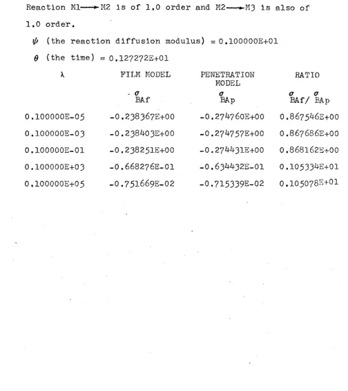
■M2 is of 1.0 order and M2-Reaction Ml—

1.0 order.

(the reaction diffusion modulus) = 0.100000E+01

9 (the time) = 0.1272?23+01

M3 is also of

0.100000E-05

0.100000E-03 0.lOOOOOE-Ol 0.100000E+03

0.100000E+05

FILM MODEL

- a

BAf

-0.238367E+00 -0.238403E+00

-0.238251E+00 -0.668276E-01

-0.751669E-02

PENETRATION MODEL

a

BAp

-0.274760E+00 -0.274757E+00

-0.274431E+00 -0.634432E-01 -0.715339E-02

RATIO

a a

BAf/ BAp

4-6

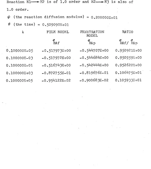
Reaction Ml-

1.0 order.

TABLE IV

■M2 is of 1.0 order and M2- •M3 is also of

ip (the reaction diffusion modulus) = 0.200000E+01

0 (the time) = 0.509090E+01

0.100000E-05 0.100000E-03 0.100000E-01 0.100000E+03 0,100000E+0 5 FILM MODEL a BAf -0.5179735+00 -0.517972E+00 -0.5l67^3E+00 -0 .8727552-01 -0.95^122E-02 PENETRATION MODEL a BAp -0.5^7075+00 -0.5^684E+00 -0.5A2^4E+00 -O.8I9676E-OI -0 .900683E-02 RATIO

a a

BAf/ BAp 0.9509215+00 0.9509595+00 0.952620E+00

0.106A75E+01

0.1059335+01

-M2 is of 1.0 order and M2-Reaction Mi­

lt 0 order.

ip (the reaction diffusion modulus) = 0.206439E+01

6 (the time) = 0.542400E+01

M3 is also of

0.100000E-05 0.100000E-03 0,100000E-01

0.100000E+03

0.100000E+05

FILM MODEL

a

BAf

-0.530950E+00 -0.53093^E+00

-0 .529600E+00

-0 .877076E -.01 -0.95840IE-02

PENETRATION MODEL

a

BAp

-0.556475E+00 -0.556451E+00

-0.554040E+00

- 0 .824698E-01 -0.905706E-02

RATIO

a a

BAf/ BAp

0.954130E+00 0.954143E+00

48

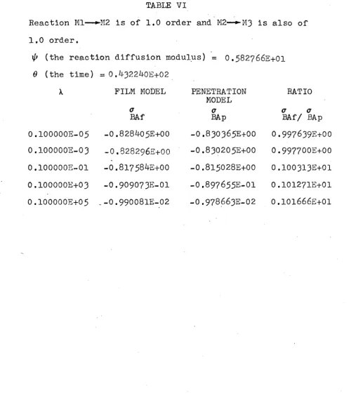
TABLE VI

Reaction Ml— ►M2 is of 1.0 order and M2— ^M3 is

1.0 order.

(the reaction diffusion modulus) = 0.582766s

6 (the time) = 0.432240E+02

0.100000E-05

0

.

E

0.100000E-01 0.100000E+03 FILM MODEL a BAf -0.828405E+00 -0.828296E+00 -0.817584E+00 -0.909073E-01

0.100000E+05 .-0.990081E-02

PENETRATION MODEL a BAp -0.830365E+00 -0.830205E+00 -0.815028E+00 -0.897655E-01 -0.978663E-02

also of

+01

RATIO

a a

BAf/ BAp 0.997639E+00 0.997700E+00 0.100313E+01 0.101271E+01 0.101666E+01

TABLE VII

-M2 is of 1.0 order and M2- -M3 is also of Reaction Mi­

lt 0 order.

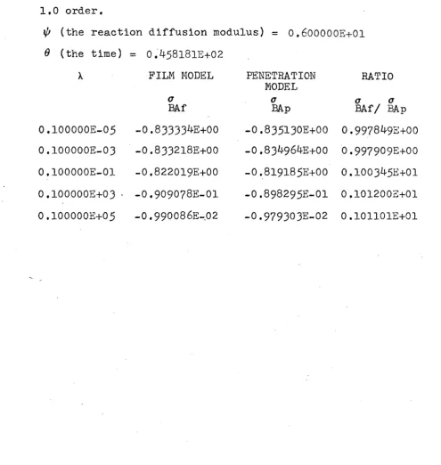
\l> (the reaction diffusion modulus) = 0.600000E+01

6 (the time) = 0.458181E+02

0.100000E-05

0.100000E-03 0,100000E-01

0.100000E+03

0.100000E+05

FILM MODEL

a

BAf

-0.833334E+00 -0.833218E+00

-0.822019E+00

-0.909078E-01 -O.99OO86E-.O2

PENETRATION MODEL

a

BAp

RATIO

a t a

BAf/ BAp -0.835130E+00 0.997849E+00 -0.834964E+00 0 .997909E+00 -0.819185E+00 0.100345E+01

-0.898295E-01 0.101200E+01

50

TABLE VIII

•M2 is of 1.0 order and M2- M3 is also of Reaction Ml

1.0 order.

ip (the reaction diffusion modulus) = 0 .100000E+02

9 (the time) = 0.127272E+03 FILM MODEL

a

BAf

PENETRATION MODEL

a

BAp

RATIO

a a

BAf/ BAp

0 .100000E-05 -o.899997E+00 0.100000E-03 -0.89^756e+00

0.100000E-01 -0.877^71E+00

0.100000E+03 -O.9O9O9OE-OI 0.100000E+05 -0.990098E-02

-0.900388E+00 0.999566E+00 -0.900059E+00 0.99^108E+00 -0.871367E+00 0.100700E+01

-0.905177E-01 0.100432E+01 -0.986185E-02 0.100396E+01

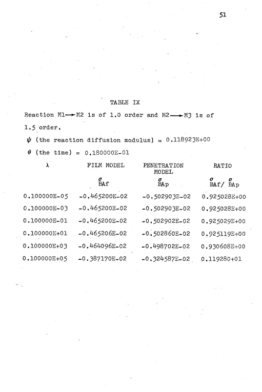
TABLE IX

Reaction Ml— ►M2 is of 1.0 order and M2 *-M3 is of

1.5 order.

ip (the reaction diffusion modulus) = O.II8923E+OO

0 (the time) = 0.180000E-01

X FILM MODEL PENETRATION

MODEL

RATIO

a a 0 0

BAf BAp BAf/ BAp

0.100000E-05 -0.if65200E-.02 -0.502903E-02 0.925028E+00

0.100000E-03 -0.465200E-02 -0.502903E-02 0.925028E+00 0.100000E-01 -0.465200E-02 -0.502902E-02 0.925029E+00

0.100000E+01 -0.465206E-02 -0.502860E-02 0.925H9E+00

0.100000E+03 -0.464096E-02 -0.498702E-02 0.930608E+00

52

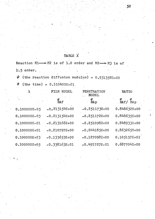
TABLE X

Reaction Ml *-M2 is of 1.0 order and M2— >- M3 is of

r. $ order.

^ (the reaction diffusion modulus) = O.931358E+OO

6 (the time) = 0 .1-lO^OOE+Ol.

0.100000E-05 0.100000E-03 0.100000E-01 0.100000E+01 0.100000E+03 O.IOOOOOE+O5 FILM MODEL. a BAf -0 ,21315^+60 -0 .21315^+00 -O.2I 3166E+OO -0 .210797E+00 -0.133653E+00 -0.338163E-01 PENETRATION . . MODEL

a BAp -0.251173E+00 -0.251172E+00 -0.251098E+00 -0.2^l85E+00 -0.127098E+00 -.0.491727E-01 RATIO

a a

. aAf/ bap .

0.8^8632E+00

0.848635E+00

0.848933E+00

O.863265E+OO

o . i 0 5 i 5 7 E + o r :

0.687704E+00

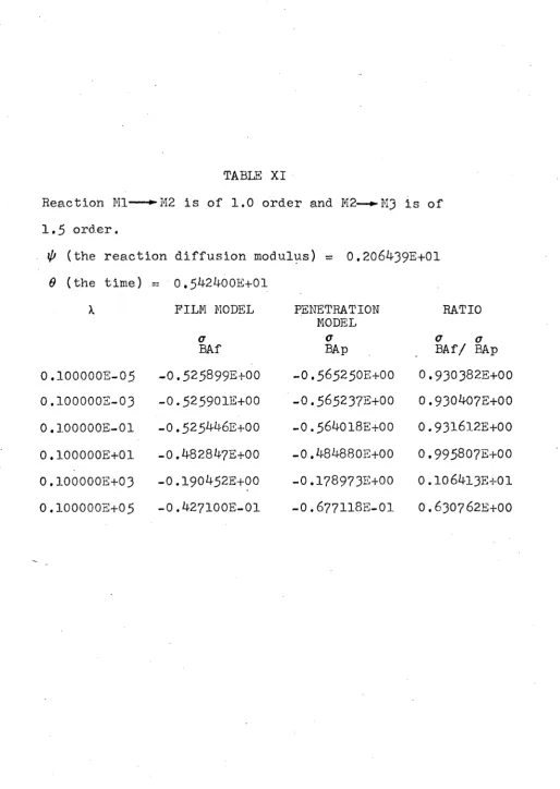
TABLE XI

Reaction Ml ► MB is of 1.0 order and M2— ► M 3 is of

1,5 order.

ip (the reaction diffusion modulus) = 0 .206^39E+01

6 (the time) = 0 ,5^2^-OOE+Ol

0.100000E-05 0.100000E-03 0.100000E-01 0.100000E+01 0.100000E+03 0.100000E+05 FILM MODEL a BAf -0.525899E+00 -0.525901E+00 -0 .525^ 6E+00

-0.^-828^?E+00 -0.190^52E+00 -0.^27100E-01 PENETRATION MODEL a BAp -O.56525OE+OO -O.565237E+OO -0.564018E+00 -0 ,^-8^880E+00 -0.178973E+00 -0.677118E-01 RATIO

o a

5 k

TABLE XII

Reaction Ml ►M2 is of 1.0 order and M2 ^M3

1.5 order.

4> (the reaction diffusion modulus) = 0.291625E+01

6 (the time) = 0.1082i|-0E+02 X 0.100000E-05 O.IOOOOOE-O3 0.100000E-01 0 ,100000E+01 0.100000E+03 0.100000E+05 FILM MODEL a BAf -0.651801E+00 -0.651808E+00 -0 .65036^+00 -0.554022E+00 -0.19^646E+00 -0.^19237E-01 PENETRATION MODEL a BAp -0.68^553E+00 -0.68^523E+00 -0 .68156^+00 -0 .541663E+00 -0.188601E+00 -0.711512E-01 is of RATIO

o a

BAf/ BAp 0 .95215^+00 0.952207E+00 0.95^222E+00 0.102281E+01 0 .103205E+01

0 .589219E +00

TABLE XIII

Reaction Ml ►M2 is of 1.0 order M2 ►M3 is of

1,5 order.

^ (the reaction diffusion modulus) = 0 .^12192E+01

6 (the time) = 0.2l62^0E+02

0.100000E-05 0.100000E-03 0,100000E-01 0.100000E+01 0.100000E+03 0.100000E+05 FILM MODEL a BAf -0.7^71932+00 >0.7^7211E+00 -0.7^37552+00 ■0.579572E+00 .0 .192977E+00 •0 .394591E-01 PENETRATION MODEL a BAp -0 .778^36e+00 -0.7783732+00 -0.772270E+00 -0.572484E+00 -0.193758E+00 -0.729936E-01 RATIO

a # a

56

TABLE XIV

Reaction Ml ►M2 is of 1.0 order and M2 ►M3 is of

1.5 order.

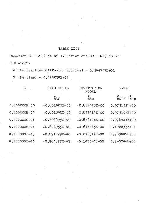
ip (the reaction diffusion modulus) = 0 .50^737E+01

6 (the time) = 0 .324239E+02

0.100000E-05 0.100000E-03 0.100000E-01 0.100000E+01 0.100000E+03 0.100000E+05 FILM MODEL a BAf .O.78927OE+OO .0.789297E+00 -0 .783962E+00 •0.582A05E+00 ■0 .190835E+00 •0.375011E-01 PENETRATION MODEL a BAp -0.822378E+00 -0.822286E+00 -0.813^81E+00 -0.583095E+00 -o.195532E+00 -0.736272E-01 RATIO

a a

BAf/ BAp 0 . 9 5 9 7 ^ + 0 0 0.959881E+00 O.963712E+OO

0.998815E+00

0.975980E+00 0.509337E+00

Reaction Ml *-M2 is of 1.0 order and M2 *-M3 is of 1.5 order.

^ (the reaction diffusion modulus) = O.582766E+OI

0 (the time)

X 0.1OOOOOE-O5 0.100000E-03 0.100000E-01 0,100000E+01 0.100000E+03 0.100000E+05 = 0.432240E+02 FILM MODEL a BAf -0.813855E+00 -0.813891E+00 -0.806852E+00 -0.581930E+00 -O.I88967E+OO -0.359067E-01 PENETRATION MODEL a BAp -0.8^93^2E+00 -0.849223E+00 -0.838019E+00 -0.588464E+00 -0.196^29E+00 -0.739^79E-01 RATIO

a a

TABLE XVI

Reaction Ml ►M2 is of 1.0 order and M2--- ►M3 is of

1.5 order.

i/'Cthe reaction diffusion modulus) = 0.683302E+01

6 (the time) = 0 .59^2i|-0E+02

0.100000E-05 0.100000E-03 0.100000E-01 0.100000E+01 0.100000E+03 0.100000E+05 FILM MODEL a BAf .O.836619E+OO -O.836562E+OO .0.827362E+00 -0 .580129E+00 .O.I8656OE+OO

•0.339^7 5E-01

PENETRATION MODEL a BAp -O.875E56E+OO -0.875301E+00 - 0 ,86093^E+00

-0.592888E+00

-0.197169E+00

-0.7^2121E-01

RATIO

a a

BAf/ BAp O.955638E+OO 0.9557^2E+00 0.961005E+00 0 .978E79E+00 0.9^6l91E+00 0.^57^393+00

TABLE XVII

Reaction Ml— ►M2 is of 1.0 order and M2

2,0 order.

^(the reaction diffusion modulus)

M3 is of

0.118923E+00

RATIO

6 (the time) =

\ O.lOOOOOE-05 0.100000E-03 0.100000E-01 0.100000E+01 0 .100000E+03 0.100000E+05 0.180000E-01 FILM MODEL a BAf -0.468774E-02 -0.468774E-02 - 0 .468774E-02

-0.465200E-02 -0.465232E-02 -0.462080E-02 PENETRATION MODEL a BAp -0.502903E-02 -0.502903E-02 -0 .502903E-02 -0.502901E-02 -0.502724E-02 -0.486582E-02

BAf/ BAp

60

TABLE XVIII

Reaction Ml— ►M2 is of 1.0 order and M2 ^M3 is of

2.0 order.

^(the reaction diffusion modulus) = 0.931358E+00

0 (the time) '=

X 0 .100000E-05 0.100000E-03 0.100000E-01 0.1000003+01 O.100000E+03 0.100000E+05 0.110^00E+01 FILM MODEL O’ BAf -0.21^88lE+00 -0.214881E+00 -0.21^-8763+00 -0.212677E+00 -0.182366E+00 -0.758907E-01 PENETRATION MODEL a BAp -0.251173E+00’ -0.251173E+00 -0.251151E+00 -0.2^9020E+00 -0.181657E+00 -0 .701529S-01 RATIO

<r a

BAf/ BAp

0.855511E+00 0.8555HE+00 0 .855566E+00 0.854056S+00 0 .100390S+01 0.108178E+01

TABLE XIX

Reaction Ml ^M2 is of 1.0 order and M2 >M3 is of

2.0 order,

^(the reaction diffusion modulus) - 0 .206^39^4-01

0 (the time) = 0 . 5^2399E-K)1

0.100000E-05 0.100000E-03 0.100000E-01 0.100000E+01 0 .100000E+03 0 .100000E+05

FILM MODE I.

a BAf -0.5309.50E+00 ■0 .5309^82+00 ■0.530738S+00 .0.507111E+00 •0.285607E+00 •0,100282E+00 PENETRATION MODEL a BAp -0.565250E+00 -0.565243E+00 -0.564618E+00 -0 .519583E+00 -0.268579E+00 -0.9^5728E-01 RATIO

a a

62

TABLE XX

Reaction Ml ►•M2 is of 1.0 order and M2 >u)3 is of

2,0 order.

ip (the reaction diffusion modulus) = 0.291625E+01

6 (the time) = 0.108240E+02

0.100000E-05 0.100000E-03 0.100000E-01 0.100000E+01 0.100000E+03 0.100000E-i-05 FILM MODEL a BAf -0 .65910^+00 -0 .659096E+00 .0 .658356E+00 -0.596959E+00 ■0.29^l89E+00 •0 .IOIO89E+OO PENETRATION MODEL a BAp -O.68E553E+OO -0.684536E+00 - 0 .682766E+00 -0.590022E+00

-0.284705E+00

-0.990919E-01

RATIO

BAf/ BAp 0 .962822E+00 0.962837E+00 0 .96i|-2L7E+00 0.101175E+01 0.103331E+01 0.102016E+01

TABLE XXI

Reaction Ml > JA2 is of 1.0 order and M2 ►M3 is of

2.0 order.

^(the reaction diffusion modulus) = 0.^12192E+01

6 (the time) = 0.2l62^0E+02

0.100000E-05 0.100000E-03

0.100000E-01

0

.

0 .100000E+03 0 .100000E+05 FILM MODEL a BAf -0.757539E+00 •0.757519E+00 -o.755^57E+oo .0 .63596IE+00

.0 .293372E +00 ■0.9875^9E-0l PENETRATION MODEL <r BAp -0.778436E+00 -0.77839^E+00 -0.77it-309E+00 -0.629165E+00 -O.293343E+OO -0.101512E+00 RATIO

BAf/ BAp