3D Reconstruction Using a Stereo Vision System with Simplified Inter-Camera Geometry

Scholarship at UWindsor

Scholarship at UWindsor

Electronic Theses and Dissertations Theses, Dissertations, and Major Papers

2010

3D Reconstruction Using a Stereo Vision System with Simplified

3D Reconstruction Using a Stereo Vision System with Simplified

Inter-Camera Geometry

Inter-Camera Geometry

Zhuo Wang

University of Windsor

Follow this and additional works at: https://scholar.uwindsor.ca/etd

Recommended Citation Recommended Citation

Wang, Zhuo, "3D Reconstruction Using a Stereo Vision System with Simplified Inter-Camera Geometry" (2010). Electronic Theses and Dissertations. 345.

https://scholar.uwindsor.ca/etd/345

This online database contains the full-text of PhD dissertations and Masters’ theses of University of Windsor students from 1954 forward. These documents are made available for personal study and research purposes only, in accordance with the Canadian Copyright Act and the Creative Commons license—CC BY-NC-ND (Attribution, Non-Commercial, No Derivative Works). Under this license, works must always be attributed to the copyright holder (original author), cannot be used for any commercial purposes, and may not be altered. Any other use would require the permission of the copyright holder. Students may inquire about withdrawing their dissertation and/or thesis from this database. For additional inquiries, please contact the repository administrator via email

by Zhuo Wang

A Thesis

Submitted to the Faculty of Graduate Studies through School of Computer Science in Partial Fulfillment of the Requirements for the Degree of Master of Master of Science at the

University of Windsor

Windsor, Ontario, Canada 2010

c

by Zhuo Wang

APPROVED BY:

Dr. Majid Ahmadi

Department of Electrical and Computer Engineering

Dr. Imran Ahmad School of Computer Science

Dr. Boubakeur Boufama, Advisor School of Computer Science

Dr. Yung H. Tsin, Chair of Defense School of Computer Science

Declaration of Co-Authorship

I hereby declare that this thesis incorporates material that is result of joint research in collaboration with Dr. Boubakeur Boufama. The collaboration is covered in Chapter 4 of the thesis. In all cases, the key ideas, primary contributions, experimental designs, data analysis and interpretation, were performed by the author, and the contribution of co-authors was primarily through the provision of guidance and criticism.

I am aware of the University of Windsor Senate Policy on Authorship and I certify that I have properly acknowledged the contribution of other researchers to my thesis, and have obtained written permission from the co-author to include the above material in my thesis.

Abstract

.

Acknowledgements

Declaration of Co-Authorship iii

Abstract iv

Dedication v

Acknowledgements vi

List of Figures ix

List of Tables xi

1 Introduction 1

2 Background 4

2.1 Projection Process . . . 4

2.2 Stereo Vision . . . 9

2.2.1 Epipolar Geometry . . . 11

2.2.2 Eight-Point Algorithm . . . 14

2.2.3 Motion Recovery . . . 16

2.2.4 Scene Reconstruction . . . 17

2.3 Conclusion . . . 18

3 Related Work 20 3.1 Classical Calibration . . . 20

3.1.1 Calibration by More Than One Images . . . 21

3.1.2 Calibration by Only One Image . . . 22

3.2 Self-Calibration . . . 23

3.3 Motion Recovery . . . 24

3.4 Scene Reconstruction . . . 25

3.5 Conclusion . . . 26

4 Error Effects on 3D Reconstruction 27

4.1 General Case: Rotation and Translation Between the Two Cameras . . . 30

4.2 Simplified Case: Pure Translation Between the Two Cameras . . . 38

4.3 Discussion . . . 47

4.4 The Use of Perpendicularity to Obtain the Focal Length . . . 48

4.4.1 Mathematical Analyze . . . 48

4.4.2 Experiment . . . 50

4.5 Conclusion . . . 51

5 Conclusion 54

Bibliography 57

2.1 Projection Process . . . 6 2.2 Stereo Vision . . . 10 4.1 Translation along X-Axis and regular rotation, with principal point

coordi-nate error and 0.5 pixel error level . . . 30 4.2 Translation along X-Axis and regular rotation, with principal point

coordi-nate error and 1.0 pixel error level . . . 31 4.3 Translation along X-Axis and regular rotation, with focal length error and

0.5 pixel error level . . . 32 4.4 Translation along X-Axis and regular rotation, with focal length error and

1.0 pixel error level . . . 33 4.5 Translation along Y-Axis and regular rotation, with principal point

coordi-nate error and 0.5 pixel error level . . . 34 4.6 Translation along Y-Axis and regular rotation, with principal point

coordi-nate error and 1.0 pixel error level . . . 35 4.7 Translation along Y-Axis and regular rotation, with focal length error and

0.5 pixel error level . . . 36 4.8 Translation along Y-Axis and regular rotation, with focal length error and

1.0 pixel error level . . . 37 4.9 Translation along X-Axis and small rotation, with principal point

coordi-nate error and 0.5 pixel error level . . . 39 4.10 Translation along X-Axis and small rotation, with principal point

coordi-nate error and 1.0 pixel error level . . . 40 4.11 Translation along X-Axis and small rotation, with focal length error and 0.5

pixel error level . . . 41 4.12 Translation along X-Axis and small rotation, with focal length error and 1.0

pixel error level . . . 42 4.13 Translation along Y-Axis and small rotation, with principal point coordinate

error and 0.5 pixel error level . . . 43 4.14 Translation along Y-Axis and small rotation, with principal point coordinate

error and 1.0 pixel error level . . . 44

4.15 Translation along Y-Axis and small rotation, with focal length error and 0.5 pixel error level . . . 45 4.16 Translation along Y-Axis and small rotation, with focal length error and 1.0

4.1 Calibration Test . . . 51

Introduction

Computer vision is the theory of retrieving, interpreting and utilizing information from a single image, multiple images or videos. Most of the time cameras are used as the devices to acquire information. Camera calibration and scene reconstruction are two important tasks in computer vision, contributing to applications of robot navigation, stereo vision, pattern recognition, video surveillance, and others. In this thesis, the pin-hole camera model is adopted: 3D (three dimensional) scene points are projected through a single point (pin-hole) to an image plane.

Camera calibration is defined as the estimation or calculation of the intrinsic parameters of a camera. The intrinsic parameters consists of the followings: the principal point (image centre) coordinates; the focal length, which is the distance between principal point and camera centre (projection centre); the aspect ratio, which is the ratio of the horizontal size and the vertical size of a single pixel in a image; and the skew factor, which describes the distortion of pixels if they are not rectangular. Currently, widely-used commercial CCD cameras can provide the features which ensure that both the horizontal size and the vertical size of a single pixel are the same and the pixel is always rectangular. Therefore, in this

thesis it is convenient to assume that the aspect ratio is 1 and the skew factor is 0.

Scene reconstruction is defined as the process of recovering 3D scene information from an image or set of images. The projection of 3D scene to a 2D (two dimensional) image is a process in which we lose one dimension [1], and some useful information has been lost during the projection. The full reconstruction, which is very important for the upcoming ap-plication, is to recover the original Euclidean structure of the scene. In order to reconstruct the Euclidean structure of the scene, additional information is required. This is difficult because the projective structure lacks metric information [4]. In other words, one cannot fully reconstruct the scene from a single image without any prior information [3]. In this thesis, scene reconstruction means the recovery of the Euclidean structure of the scene.

manufacturer’s data or previous experiments [4, 5]. Consequently once the pure translation is performed, the calibration can be totally avoided during the 3D reconstruction task.

If the motion is restricted as described before, the projection can be dramatically sim-plified since the rotation matrix is identity. It brings a neat expression of scene point coordi-nates in three directions, respectively, from intrinsic parameters and corresponding pixels. This turns the complicated camera calibration into a simple task: any geometry constraint in the scene can be applied if there is a constraint which can form sufficient equations to solve unknowns. In this thesis we propose a calibration method by applying the perpendic-ular constraint as an example. The output of such method is a single linear equation of three unknowns: focal length and two principal point coordinates. Any unknown parameter can be calculated if the other two parameters are known. It is suggested to use the perpendicular constraint for computing the focal length, since the principal point coordinates are almost equal to the centre of the image in modern CCD cameras. Some parts of this thesis have been published [51].

Background

This chapter’s aim is to introduce the prerequisite and fundamental concepts for camera calibration and scene reconstruction. It is divided into two parts: first, the illustration and the mathematical expression of the projection process is provided; next, stereo vision is in-troduced. In stereo vision, the general expression set to describe ”stereo” is demonstrated. Then, because of the stereo feature, epipolar geometry is described in short. Derived from this epipolar geometry, an eight-point algorithm and a motion recovery algorithm are intro-duced. Once all of this is finished, it is straightforward to show how to recover the Euclidean structure of a scene.

2.1

Projection Process

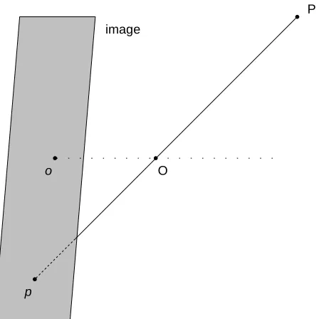
A camera is a device which can project a 3D scene onto a 2D image. Since the pine-hole model is a good approximation of the real camera, the camera concept in this thesis is the pin-hole model assumption. Suppose all light rays are straight line, ”pin-hole” means every ray should go through a single point, which lies in front of the inner part of the camera.

This single point is called ”pin-hole” or camera centre.

The whole projection process can be divided into three different steps:

The first step is a 3D rigid transformation. This transformation changes the 3D coor-dinate system from the scene coorcoor-dinate system to the camera coorcoor-dinate system, whose origin is the same as the camera origin. Such a centre is denoted asO. The camera origin Ois also called “the projection centre”. This step can be avoided if the scene coordinate system is the same as the camera coordinate system, sometimes practical when the scene coordinate system is totally unknown.

The second step is a 3D to 2D transformation. The 3D scene is projected onto a camera frame through the projection centre O. A light ray between any 3D scene point and its corresponding camera frame point must go throughO. Note that a camera frame point is a 2D point, and its coordinate system is the same as the camera coordinate without the depth axis (generally notedZ). The distance between the frame and the camera centre is the focal length. The boundary of a camera frame is infinite.

The last step is a 2D to 2D transformation. The goal of this step is to obtain the final image, which is acquired from the camera frame. This transformation changes the 2D coor-dinate, from the frame coordinate to the image coordinate. The image coordinate consists ofuaxis, vaxis and the origin. If there is a line along theZ axis that goes throughO, this line will intersect a camera frame. This intersection point, under the image coordinate, is called ”image centre” and denoted aso. Note that this transformation is not a rigid one: it is an affine transformation.

P

O o

p

image

By using a homogeneous coordinate, the scene pointPcan be expressed as the vector P= (X,Y,Z,T)T and the image pointpcan be expressed as the vectorp= (u,v,τ)T. From

now on, if a scene point is described under the original scene coordinate system rather than the camera coordinate system, it is denoted as ˜P; if a scene point is described under the camera coordinate system rather than the scene coordinate system, it is denoted as P. Similarly, if a 2D point is on a camera frame and is described under a camera frame

coordinate, it is denoted as ˜p; if a 2D point is on a camera frame and is described under an image coordinate, it is denoted asp.

The first transformation, which is a 3D rigid transformation, can be expressed with the equation:

P=DP˜ (2.1)

whereDis a 3D transformation matrix that describes the transformation from the scene coordinate system to the camera coordinate system. When considering the second trans-formation, which is a 3D to 2D projection transtrans-formation, Equation (2.1) will be changed to:

˜

p=IP=IDP˜ (2.2)

whereI is a 3D to 2D projection matrix. Finally when the last step, a 2D to 2D coordi-nate system transformation is under consideration, the expression will be:

p=Ap˜=AIP=AIDP˜ (2.3)

This coordinate transformation is an affine transformation. A is also called ”the intrinsic matrix”. It describes the intrinsic parameters of the camera. The details of this matrix are shown below: A=      

αu 0 u0

0 αv v0

0 0 1

      (2.4)

whereαu, αvare image scale factors andu0,v0are image centre coordinates under the

image coordinate system. What’s more,αu=−f ku andαv =−f kv, where f denotes the focal length of the camera,ku denotes the ratio between pixel coordinate unit and camera coordinate unit along u axis, and kv denotes the ratio between pixel coordinate unit and camera coordinate unit alonguaxis. Sometimesαu andαv are also called ”focal length”, and it is applied in the following context. If the scene coordinate can be set as the same as the camera coordinate,Dwill be an identical matrix andP=P. If˜ T andτare set to be 1, a

scale factorλwill be introduced. Therefore, due to the introduction ofλ,Ican be expressed

as I=      

1 0 0 0 0 1 0 0 0 0 1 0

      (2.5)

The overall projection equation will be:

p=λAIP (2.6)

      u v 1       =λ      

αu 0 u0

0 αv v0

0 0 1

           

1 0 0 0 0 1 0 0 0 0 1 0

               X Y Z 1          (2.7)

2.2

Stereo Vision

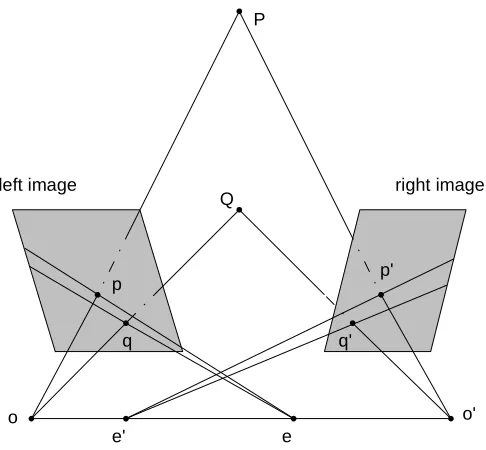
This section deals with the situation when there are two cameras with a fixed configuration. It is convenient to assume that the coordinate of one camera can be adopted as the 3D scene coordinate. For simplicity, the reference camera is called the ”left camera” and another camera is called the ”right camera”. Assume that there is a scene point that can be projected into both cameras and can be observed in both images, then the 3D coordinate of this point can be recovered. This process is called scene reconstruction. See Figure 2.2. Note that images are placed in front of the camera centre, which is to facilitate analysis: the image acquired no longer represents an upside down scene.

In order to simplify this problem, it is appropriate to suggest that these two cameras are identical, meaning their intrinsic parameters are the same. Suppose that there is a scene pointP, based on the previous discussion with one camera, the equation set can be easily formed to describe the projection process with two cameras:

  

 

p=λAIP

p0=λ0AI0P

(2.8)

left image right image P

o

Q

o' p

q

p'

q'

e' e

I0= (R|t), whereRis the rotation matrix andt = (tX,tY,tZ)T is the translation vector. R=      

R₁₁ R₁₂ R₁₃

R21 R22 R23

R31 R32 R33       (2.9)

The details of Equation (2.8) is shown below:

                                                 u v 1       =λ      

αu 0 u0

0 αv v0

0 0 1

           

1 0 0 0 0 1 0 0 0 0 1 0

               X Y Z 1                u0 v0 1      

=λ0      

αu 0 u0

0 αv v0

0 0 1

           

R11 R12 R13 tX

R21 R22 R23 tY

R31 R32 R33 tZ

               X Y Z 1          (2.10)

2.2.1

Epipolar Geometry

Figure 2.2 also illustrates the so-called “epipolar geometry” [40]. If there exists two cam-eras, along the epipolar line, their centresOandO0, respectively, can be determined. Sup-pose there are two scene points P and Q, and both of them can be projected onto each image, the corresponding projected points can be noted asp,qon the left image, and p0,q0 on the right image. It is well-known that light rays travel in a straight line, so that plies on the linePO. Similarly,q, p0andq0lie on the linesQO,PO0andQO0, respectively.

if lines are represented by vectors, the cross product of vectorsOO~ 0andOp~ is perpendicular to the vectorO~0p0. The expression is:

~

O0p0·(O~0O×Op~ ) =0 (2.11) where·denotes scalar product and×denotes cross product. Equation (2.11) is correct if all the elements are defined in the same coordinate system. Suppose the coordinate system of one camera is selected as the reference, and denoteO~0P0 as ˜p0T, O~0Oast andOp~ as ˜p. Equation (2.11) turns into:

˜

p0T·(t×Rp˜) =p˜0TT RP=0 (2.12) whereRis the rotation matrix andt×=T, whereT is the anti-symmetric matrix:

t×=T =



    

0 −tZ tY tZ 0 −tX

−t_Y t_X 0



    

(2.13)

Here a new matrixE=T Ris adopted.Eis called the “essential matrix”. Then Equation (2.12) becomes

˜

p0TEp˜=0 (2.14)

ax+by+c=0 (2.15)

Equation (2.15) is a line equation. Therefore, it demonstrates that pointp0lies on a line formed byEp. This is the inner connection between two image points projected from a˜ single scene point: if each of the two points is determined, the position of another point can be limited on a line. This is also called “epipolar constraint” or “Longuet-Higgins constraint”. This constraint can be used to find the corresponding point in another image if one feature point in one image is selected.

Point p and point p0, which are discussed above, are defined within the normalised coordinates, which means these two points are defined under a camera frame coordinate system. In order to transform from normalised coordinates to pixel coordinates, which means these two points are defined under image coordinate system, the intrinsic matrixA should be introduced. If point p and point p0 are defined under pixel coordinate system, since ˜p=A−1pand ˜p0=A0−1p0, Equation (2.15) becomes

(A0−1p0)TE(A−1p) =0 (2.16)

Then

p0TA0−TEA−1p=0 (2.17)

Here we introduce a new matrix F =A0−TEA−1 called “fundamental matrix”. Then Equation (2.17) turns into:

2.2.2

Eight-Point Algorithm

As shown in Equation (2.18), the fundamental matrixF can be determined by p and p0. Denote that p=u,v,1T and p0=u0,v0,1T. Equation (2.18) turns into:

p0F p=

      u0 v0 1            

F11 F12 F13

F21 F22 F23

F31 F32 F33             u v 1      

=0 (2.19)

That is:

uu0F11+uv0F21+uF31+vu0F12+vv0F22+vF32+u0F13+v0F23+F33=0 (2.20)

A f =            

u1u01 u1v01 u1 v1u01 v1v01 v1 u01 v01 1

u₂u0₂ u₂v0₂ u₂ v₂u0₂ v₂v0₂ v₂ u0₂ v0₂ 1 u₃u0₃ u₃v0₃ u₃ v₃u0₃ v₃v0₃ v₃ u0₃ v0₃ 1 ..

. ... ... ... ... ... ... ... ... u_nu0_n u_nv0_n u_n v_nu0_n v_nv0_n v_n u0_n v0_n 1

                                      F11 F21 F31 F₁₂ F₂₂ F₃₂ F₁₃ F23 F33                          

=0 (2.21)

where f contains all elements of the matrixF andAis the equation matrix. SinceF and f are defined up to an unknown scale, the additional constraint of forcing the norm of f to be 1 can be made. Therefore, thanks to this additional constraint, eight points, which can form eight equations, are sufficient to solve Equation (2.21). Some algorithms, such as Jacobi or Singular Value Decomposition (SVD), can be applied to find the least eigenvector ofATA. The found eigenvector is the solution. Another method of solving Equation (2.21) is to setF₃₃ =1, which turns it into a linear least squares minimisation problem. It is claimed that general conclusions from these two algorithms, additional constraint and mandatory normalisation, are equally valid [20].

homogeneous coordinates be unity. Another is by scaling the translation to minimise the value of coordinates. In practice, there are two approaches for improvement: isotropic scaling and non-isotropic scaling. As described in [20], these two approaches are listed below:

Isotropic Scaling:

1. The points are translated so that their centroid is at the origin.

2. The points are then scaled so that the average distance from the origin is equal to√2. 3. This transformation is applied to each of the two images independently.

Non-isotropic Scaling:

1. The points are translated so that their centroid is at the origin.

2. Both of two principal moments become unity by applying Choleski factorisation.

2.2.3

Motion Recovery

Once the essential matrix E is acquired, it is possible to decompose it and to recover the rotation and translation elements. Due to [31],E=RT, whereRis the rotation matrix and T is the translation matrix. The outline of the algorithm can be found in [22]:

1. FindE.

2. Find the SVD ofE=U DVT, whereD=diag(a,b,c)anda≥b≥c.

(U ZVT|U(0,0,1)T) (U ZVT| −U(0,0,1)T) (U ZTVT|U(0,0,1)T) (U ZTVT| −U(0,0,1)T)

where Z=      

0 1 0

−1 0 0

0 0 1

      (2.22)

To select the correct motion matrix, randomly select one point pair and test if the recon-structed scene point is in front of the camera.

2.2.4

Scene Reconstruction

Suppose the intrinsic parameters, the rotation matrix and the translation matrix are known, as shown in Equation (2.10). It is straightforward then to reconstruct the scene. Suppose there is a matrixM=AI. The projection equation, Equation (2.3), turns into:

      u v 1       =λ      

m11 m12 m13 m14

m21 m22 m23 m24

m31 m32 m33 m34                X Y Z 1          (2.23)

  

 

u= m11X+m12Y+m13Z+m14

m31X+m32Y+m33Z+m34

v= m21X+m22Y+m23Z+m24

m31X+m32Y+m33Z+m34

(2.24)

For a pair of image pointsp= (u,v,1)T and p0= (u0,v0,1)T:

                

u=m11X+m12Y+m13Z+m14

m31X+m32Y+m33Z+m34

v=m21X+m22Y+m23Z+m24

m31X+m32Y+m33Z+m34

u0= m011X+m120 Y+m013Z+m014

m0₃₁X+m0₃₂Y+m0₃₃Z+m0₃₄

v0= m

0

21X+m022Y+m023Z+m024

m0₃₁X+m0₃₂Y+m0₃₃Z+m0₃₄

(2.25)

The final format of Equation (2.25) is:

        

um31−m11 um32−m12 um33−m13

vm31−m21 vm32−m22 vm33−m23

u0m0₃₁−m0₁₁ u0m₃₂0 −m0₁₂ u0m0₃₃−m0₁₃ v0m0₃₁−m0₂₁ v0m₃₂0 −m0₂₂ v0m0₃₃−m0₂₃

               X Y Z       =         

m14−um34

m24−vm34

m0₁₄−u0m0₃₄ m0₂₄−v0m0₃₄

         (2.26)

Equation (2.26) is an over-determined equation and is easily solved.

2.3

Conclusion

This chapter introduces the foundation of this field. If the intrinsic parameters are known and two images are given, the whole reconstruction process can be summarized as:

1. Find eight image point pairs.

3. Calculate the essential matrix.

4. Decompose the essential matrix to obtain rotation and translation information.

5. Reconstruct the scene.

Related Work

The camera calibration and scene reconstruction have been studies for more than two decades. This chapter is to introduce these previous works. They can be divided into several categories: classical calibration, self-calibration, motion recovery and scene reconstruction with known intrinsic parameters, which are directly related to our work. The calibration is to calculate intrinsic parameters of a camera. There are two directions: the classical calibration and self-calibration. The classical calibration uses a well known pattern while self-calibration uses matched pixels across many images instead. Motion recovery is to re-cover the configuration between two cameras. Scene reconstruction is to rere-cover the scene information.

3.1

Classical Calibration

Camera calibration is the process of calculating the intrinsic parameters of a camera. Sup-posing that not only accurate scene point coordinates, but also accurate corresponding pixel point coordinates can be acquired, and the scene coordinate system is the same as the

era coordinate system, one scene point and its projected image point can provide two equa-tions. Because the intrinsic parameters contain four elements, at least two points can pro-vide sufficient information to calculate the intrinsic parameters. The straightforward way to solve it is to use the Direct Linear Transformation method. However, it is not practical since measuring the coordinates is costly. Hence many alternative approaches have been proposed to deal with this problem. Some require more than one image; others require only one image to calibrate the camera.

3.1.1

Calibration by More Than One Images

One direction is to use a calibration pattern. Let the camera take two or more pictures from a pattern, then calculate the intrinsic parameters by measuring the predefined pattern features, which should appear in the image. This requires a, specially designed pattern, which limits its application range.

A coplanar grid can be used as a pattern to calibrate the camera. Tsai [48, 49] proposed a calibration method which recovers the intrinsic and extrinsic parameters by making them best fit the measured image coordinates of known target point coordinates. This method has two stages. The first stage is to estimate extrinsic parameters (the rotation and the translation parameters related to the scene coordinate system) by closed form least squares estimation. The second stage is to estimate intrinsic parameters by applying an iterative non-linear optimization.

many images, at least 15 to 20 images with different orientation, to achieve the promising accuracy, which limits its usage. Besides, the special designed pattern also restricts appli-cable fields. The advantage of this method is its accuracy. This method currently has been widely applied and many people use this method as the reference to test the accuracy of their proposed new methods.

3.1.2

Calibration by Only One Image

Calibration by only one image has been in development for many years. It can be divided into several categories: calibration based on vanishing points, calibration based on circles, calibration based on symmetry and calibration based on four coplanar control lines. How-ever, these methods require the specific structure of the scene and besides, the accuracy of these calibration methods is worse than the calibration method by patterns [57, 58].

The first idea of adopting vanishing points to calibrate the camera was proposed by Caprile [6]. It is based on the view of a cube. Three vanishing points can be retrieved from the image of the cube and the intrinsic parameters can be calculated from the attribute of vanishing points. Extended work has been proposed [17, 45, 53, 54, 55, 1, 9, 16]. For example, the use of an orthogonal wedge, which is defined as two rectangular planes inter-secting at right angles, as a reference structure [45]; using paralelepipeds rather than cubes, which are a subclass of parallelepipeds, to calibrate the camera [53, 54, 55]; using a single image containing a rectangular prism, which is to generate two vanishing points for camera calibration [1].

no distortion and square pixels are made. A similar attempt is proposed by [46]: camera calibration from a single view which contains three spheres. Another method was proposed by [7]: camera calibration with two arbitrary coplanar circles, even if the centres of the circles and/or part of the circles are occluded. Besides, the work of [27] was proposed as the improvement of [12]: camera calibration by using planar pattern of pairs of concentric circles. What’s more, the work of [8] was proposed: camera calibration with two arbitrary coaxial circles.

Other attempts were also proposed. The idea of using symmetry in a single image to calibrate the camera was proposed by [26]. There are three different categories from this idea. The first is calibration from translational symmetry. The second is calibration from reflective symmetry. The last is calibration from rotational symmetry. Also a method of camera calibration from a single view with four coplanar control lines was proposed by [42], who use control lines rather than control points to perform constraints. These constraints can be used to compute intrinsic parameters.

3.2

Self-Calibration

pa-rameters [50, 38].

Another approach for self-calibrating a camera consists in upgrading the projective structure of a scene into an affine one from which the metric reconstruction can be eas-ily obtained. This can be achieved by calculating the position of the plane at infinity in space either through the so-called modulus constraint [37, 18] or from a quasi-affine re-construction [24, 36]. Unfortunately, the accuracy of the estimated parameters, when using the above mentioned methods and others [14, 35], is undermined by the correspondence problem and by the numerous degenerate motion configurations [28, 44]. Since camera self-calibration is a non-linear problem, the problem of choosing initial values of parame-ters is often difficult.

In addition, initializing the optimization procedures which are close to the ground truth does not guarantee the convergence to the desired solution. For example, when the candi-date plane at infinity contains one of the camera centres, the optimization procedure fails even if the motion of the camera is not degenerated. In order to circumvent these issues, [15] have proposed a globally convergent method that uses interval analysis in order to bound the values of the camera parameters. However, the prohibitive running time of this method makes it inappropriate for most applications.

3.3

Motion Recovery

eight-point algorithm. Once the essential matrix is obtained, by using an SVD algorithm, the rotation matrix and the translation matrix can be retrieved [31, 39, 22]. Nevertheless, this algorithm is to be criticized as extensively sensitive to noise in the specification of the matched points [20]. Therefore, other but more complicated algorithms have been proposed for calculating the fundamental matrix [56, 34, 23, 2].

Then Hartley [20] improved the eight-point algorithm by adopting the idea of normal-ization. This improvement does not only make the algorithm be less sensitive to pixel error, but also make the algorithm be less sensitive to errors on the intrinsic parameters. By adopting this improved algorithm, the scene reconstruction can achieve the considerable accuracy [4]. Hence this algorithm is applied in this thesis.

3.4

Scene Reconstruction

Scene reconstruction is to recover the Euclidean information of the scene, which is of great value in computer vision [4]. The classical and most popular approach is based on known or roughly known intrinsic parameters. Once intrinsic parameters are known, the 3D structure can be recovered from matched points only [31].

motion (rotation and translation) and ten for the intrinsic parameters of the two cameras (assuming different cameras). On the other hand, using pixel correspondences yields only 7 independent constraints. [33]. Adding more images will not provide enough constraints for this problem when each new image has different intrinsic parameters. Therefore, in the general case, it is not possible to recover the Euclidean structure using only pixel corre-spondences across images. In accordance with the above this thesis uses classical scene reconstruction, which requires a priori calibration process to acquire intrinsic parameters.

When dealing with the situation where the intrinsic parameters are approximately known, it is still possible to solve the reconstruction problem [4]. The 3D reconstruction obtained this way is affected by both pixel accuracy and errors on the intrinsic parameters’ values. Although inaccurate intrinsic parameters might not be as serious as high-level pixel errors, the effect of errors in intrinsic parameters still needs to be analyzed.

3.5

Conclusion

Error Effects on 3D Reconstruction

From the previous discussion, it is obvious that the scene reconstruction process is affected by errors from pixels and intrinsic parameters. Both of these two kinds of errors are in-evitable. Besides, similar to the white noise, the values of pixel error are random and impossible to predict, which makes their influence permanent. When regarding errors in in-trinsic parameters, sometimes the inin-trinsic parameters approximation is known, either from manufacturer’s data or previous experiments. Because intrinsic parameters do not directly and independently affect the scene reconstruction result, it is possible to reduce or even eliminate intrinsic parameter errors, for the reconstruction result.

The first step in solving this problem is reviewing the scene reconstruction equation: Equation (2.6):

˜

p=λAIP˜

To help facilitate analysis, it is convenient to assume that image pixels are error free. Considering the effect of errors in intrinsic parameters, the equation above can be reformed

to:

p+p_e=λ(A+Ae)IP

=λAIP+λAeIP

whereA_e is the error matrix of intrinsic parameters and p_e is the error vector of pixel coordinates. The above equation can be reformed as:

p_e=λAeIP (4.1)

It’s obvious thatI, the projection matrix, plays an essential role in the intrinsic param-eters error influence. In order to demonstrate how motion and intrinsic paramparam-eters error corrupt the recovered scene, some simulations have been conducted. The reason for using simulations rather than real experiments is that experimental coefficients can be controlled. Without such absolute control, due to the unpredictable nature of pixel error, one cannot tell which coefficient conducts or dominates the final imperfect result. Therefore, no con-clusions can be made.

image centre and is perpendicular to the image plane.

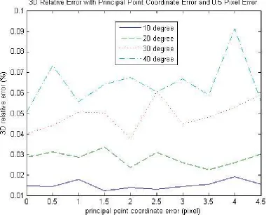
To make an acceptable approximation, the coefficients of simulation are listed as fol-lows: the pre-defined virtual scene consists of 50 random space points, which are inside a volume of 30cm(X) by 30cm(Y) by 5cm(Z); two virtual cameras are located at 20cm(Z) off the scene; for each designated inter-camera configuration, two images are created by projecting the scene into two cameras, respectively. These two images are then used as inputs for the scene reconstruction system. In addition, pixel error with 0.5 pixel level or 1.0 pixel level are added to projected image points. For every test, a total of 100 trials is carried out. For every trial, 3D space points are selected randomly and errors from pixels and intrinsic parameters are generated randomly, too. The results shown on the different graphs are obtained by taking the mean value for each case. The scenario of the simulation is the same as described in Conclusion part of Chapter 2.

Figure 4.1: Translation along X-Axis and regular rotation, with principal point coordinate error and 0.5 pixel error level

4.1

General Case: Rotation and Translation Between the

Two Cameras

First, the translation between each camera is set to be 20cmalong the X-Axis. The results are listed below:

Figure 4.5: Translation along Y-Axis and regular rotation, with principal point coordinate error and 0.5 pixel error level

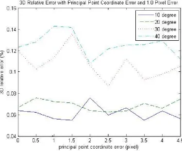
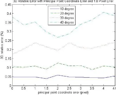
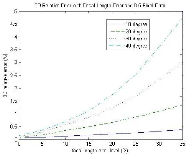
affect the overall reconstruction quality. However, it still can be concluded that most of the time smaller rotation angles yield better reconstruction quality. Figure 4.3 and Figure 4.4 show experimental results with various rotation angles and a constant translation along the X-Axis if focal length error is applied. For these two figures, the trend is very clear: the larger the rotation angle, the higher the error on the 3D reconstruction. In conclusion, the reconstruction quality drops if the rotation angle increases.

Figure 4.5, Figure 4.6, Figure 4.7 and Figure 4.8 also verify the conclusion that the bigger the rotation, the worse the reconstruction quality.

4.2

Simplified Case: Pure Translation Between the Two

Cameras

As discussed above, the rotation angles between the two cameras amplify the effect of errors on reconstruction quality. It is quite straight-forward to think about the situation when the motion is pure translation. Simulations have been performed under this situation. Coefficients are kept the same.

Figure 4.9, Figure 4.10, Figure 4.13, Figure 4.14, Figure 4.11, Figure 4.12, Figure 4.15 and Figure 4.16 again demonstrate the discipline: the smaller the rotation angle, the better the reconstruction quality. More interesting is if the rotation is totally avoided, the recon-struction quality is best and errors in the intrinsic parameters seem to be not affected by the reconstruction quality. It is illustrated in all of these figures. It is because the projection ma-trixI plays an essential role in scene reconstruction and this matrix is directly determined by the inter-camera configuration. When there is no rotation,Iis:

I=



    

1 0 0 0 1 0 0 0 1

|t



    

(4.2)

parameters also do not affect the reconstruction quality if pure translation is applied.

4.3

Discussion

The simulation result verifies the initial guess: camera motion (inter-camera configuration) plays an important role in determining how much error will corrupt the reconstruction qual-ity. This is because, as shown from above, that a large rotation will significantly amplify the noise effect derived from the pixel error or errors in intrinsic parameters. When a pure translation along the X-Axis or Y-Axis or their combination is applied, errors in intrinsic parameters will no longer affect the reconstruction quality.

Simulations were also conducted when the translation is set to the combination of move-ment along the X-Axis and movemove-ment along the Y-Axis, and the results verify the same trend. However the reconstruction quality is worse when the combined translation is ap-plied under the same conditions. This is reasonable since pure translation along the X-Axis or the Y-Axis only introduces one unknown into the matrixI, but the combined translation introduces two unknowns. Hence in the next chapter, when referring to the pure translation, it means the translation along the X-Axis or the Y-Axis separately.

4.4

The Use of Perpendicularity to Obtain the Focal Length

4.4.1

Mathematical Analyze

As discussed previously, pure translation should be applied. This section introduces another benefit when pure translation is introduced. The assumptions of ˜f =αu=αvand identical cameras are made. Since translation along the X-Axis or the Y-Axis is symmetrical, only translation along the X-Axis and Y-Axis is analyzed in detail. Equation (2.10) becomes:

                                                 u v 1       =λ      

αu 0 u0

0 αv v0

0 0 1

           

1 0 0 0 0 1 0 0 0 0 1 0

               X Y Z 1                u0 v0 1      

=λ0      

αu 0 u0

0 αv v0

0 0 1

           

1 0 0 t_X 0 1 0 0 0 0 1 0

               X Y Z 1          (4.3)

After transformation, the above equation becomes:

          

X=tX(a+bu0)

Y =c+bv0

Z=−bt_Xf˜

(4.4)

where

a=−2u

2_−2uu0_{+ (v−v}0₎2

b= u−u

0

(u−u0)2_{+ (v−v}0₎2

c=− (u−u

0_)(v+v0₎

2(u−u0)2_+2(v−v0₎2

Equation (4.4) is the overall expression of a scene point. To find out a scene point its image pair, the translation distance and intrinsic parameters are required. The scene point can also be used as a framework to calibrate the camera. Using certain space geometry constraint can form new equations, whose coefficients are image pairs, translation distance and intrinsic parameters. Since image pairs are easily known, the relationship among trans-lation distance and elements of intrinsic parameters can be obtained. Sometimes transtrans-lation distances can be eliminated and the unknowns are elements of intrinsic parameters only, which provide some methods of calculating intrinsic parameters (camera calibration).

Here the perpendicular constraint is adopted as an example. Given three scene points P1,P2andP3, each with different depth, andP~1P2andP~1P2are perpendicular, then

~

P1P2·P~2P3=0

which is

(X₂−X₁)(X₃−X₂) + (Y₂−Y₁)(Y₃−Y₂) + (Z₂−Z₁)(Z₃−Z₂) =0 (4.5) Use Equation (4.4) and Equation (4.5) turns to:

where

a0= (b₁−b₂)(b₃−b₂)

b0= (c₁−c₂)(b₃−b₂) + (c₃−c₂)(b₁−b₂)

c0= (b1−b2)(b3−b2)

d0= (a1−a2)(b3−b2) + (a3−a2)(b1−b2)

e0= (a₁−a₂)(a₃−a₂) + (c₁−c₂)(c₃−c₂)

Equation (4.6) has three unknowns: the focal length and two principal point coordinates. This shows that with a right angle in a scene, any intrinsic parameter can be calculated if the other two are previously known. As discussed before, it is convenient to assume that the principal point lies at the centre of the image. Under this assumption once the image size, which is easily fetched, is measured, the focal length can be calculated if there is a right angle existing in the scene. In the real world, right angles are common, such as windows, desks, walls and so on. Therefore, this method can be widely applied.

4.4.2

Experiment

from images, respectively. The camera is previously calibrated by Zhang’s Method [58]. The result is shown in Table 4.1. Note that values in entries have been rounded off to one decimal.

Table 4.1: Calibration Test

Test Image Position Right Angle Focal Length Reconstruction Average Error

1 Left 6 _ABC

Right 6 _{abc 2132.4 11.1mm}

2 Left 6 _DEF

Right 6 _{def 2031.3 11.7mm}

Zhang’s Method 2242.4 10.3mm

The proposed calibration method provides similar results when compared to the wide-accepted Zhang’s Method. The Zhang’s method provides a more accurate focal length since its reconstruction quality is the best. It is because the focal length obtained from Zhang’s method, which is shown in the table, is calculated by using 20 images.

Our method also works when there is only one camera: move the camera along a straight line and take two images for the scene. The length of the movement does not matter. However, in the future the proposed method still needs to be improved since its effectiveness relies on the accuracy of image point coordinates.

4.5

Conclusion

Conclusion

In this thesis we have addressed camera calibration, 3D Euclidean scene reconstruction and how inter-camera geometric configuration of a stereo vision system affects the accuracy of 3D reconstruction. We have reviewed two different calibration approaches together with motion recovery and two categories of scene reconstruction. When the intrinsic parameters and the stereo vision system geometry are unknown and there is no additional information about the scene, it is impossible to recover the 3D Euclidean structure of the scene. Note that it is possible to recover the 3D projective structure of a scene using only matched pix-els. However, such 3D reconstruction lacks any metric information making useless for most applications. In order to obtain the 3D Euclidean reconstruction, one needs to know both the intrinsic parameters and the stereo vision system’s geometry, namely, total calibration. Typically, one needs to first calibrate each camera of the stereo vision system before being able to perform the Euclidean 3D reconstruction of an observed scene. In the case of known intrinsic parameters, numerous methods have been proposed in the literature for 3D recon-struction using stereo images. However, the most reliable method that uses two images is the normalized (improved) eight-point algorithm. Therefore, in this thesis the process of

scene reconstruction consisted of the following steps. The calculation of the fundamen-tal matrix and the essential matrix is done by the improved eight-point algorithm. Then, we recover the camera configuration before performing the reconstruction of the scene by reversing the projection process. Most of the time an approximation of the intrinsic pa-rameters is easy to be acquired. Hence, we have investigated how errors in the intrinsic parameters affect the reconstruction quality and what kind of inter-camera geometry would be desirable in order to minimize the effects of these errors on the reconstructed scene.

[1] N. Avinash and S. Murali. Perspective geometry based single image camera calibra-tion. Journal of Mathematical Imaging and Vision, 30(3):221–230, 2008.

[2] P.A. Beardsley, A. Zisserman, and D.W. Murray. Navigation using affine structure from motion. Lecture Notes in Computer Science, 801:85–96, 1994.

[3] S.B. Boubakeur. On the recovery of motion and structure when cameras are not calibrated. International Journal of Pattern Recognition and Artificial Intelligence, 13(5):735–759, 1999.

[4] B. Boufama and A. Habed. Three-dimensional structure calculation: achieving accu-racy without calibration. Image and Vision Computing, 22(12):1039–1049, 2004.

[5] B. Boufama and A. Habed. Three-dimensional reconstruction using the perpendic-ularity constraint. In Sixth International Conference on 3-D Digital Imaging and Modeling, pages 241–248, 2007.

[6] B. Caprile and V. Torre. Using vanishing points for camera calibration. International Journal of Computer Vision, 4(2):127–139, 1990.

[7] Q. Chen, H. Wu, and T. Wada. Camera calibration with two arbitrary coplanar circles. Lecture Notes in Computer Science, pages 521–532, 2004.

[8] C. Colombo, D. Comanducci, and A. Del Bimbo. Camera calibration with two arbi-trary coaxial circles. Lecture Notes in Computer Science, 3951:265, 2006.

[9] J. Deutscher, M. Isard, and J. MacCormick. Automatic camera calibration from a single manhattan image. Lecture Notes in Computer Science, pages 175–188, 2002.

[10] O. Faugeras. What can be seen in three dimensions with an uncalibrated stereo rig? In G. Sandini, editor,Proceedings of the 2nd European Conference on Computer Vision, Santa Margherita Ligure, Italy, pages 563–578. Springer-Verlag, May 1992.

[11] O.D. Faugeras, Q.T. Luong, and S.J. Maybank. Camera self-calibration: Theory and experiments. In G. Sandini, editor,Proceedings of the 2nd European Conference on Computer Vision, Santa Margherita Ligure, Italy, pages 321–334. Springer-Verlag,

May 1992.

[12] V. Fremont and R. Chellali. Direct camera calibration using two concentric circles from a single view. InInternational Conference on Artificial Reality and Telexistence, pages 93–98, 2002.

[13] A. Fusiello. Uncalibrated euclidean reconstruction: A review. Image and Vision Computing, 18(6-7):555–563, May 2000.

[14] A. Fusiello. A new autocalibration algorithm: Experimental evaluation. In W. Skar-bek, editor, Computer Aanalysis of Images and Patterns, volume 2124 of Lecture Notes in Computer Science, pages 717–724. Springer-Verlag, 2001.

[16] L. Grammatikopoulos, G. Karras, and E. Petsa. An automatic approach for camera calibration from vanishing points. ISPRS Journal of Photogrammetry and Remote

Sensing, 62(1):64–76, 2007.

[17] E. Guillou, D. Meneveaux, E. Maisel, and K. Bouatouch. Using vanishing points for camera calibration and coarse 3D reconstruction from a single image. The Visual Computer, 16(7):396–410, 2000.

[18] A. Habed and B. Boufama. Camera self-calibration from bivariate polynomial equa-tions and the coplanarity constraint. Image and Vision Computing, 24(5):498–514, 2006.

[19] M. Han and T. Kanade. Creating 3D models with uncalibrated cameras. InFifth IEEE Workshop on Applications of Computer Vision, pages 178–185, 2000.

[20] R. Hartley. In defence of the eight-point algorithm. IEEE Transactions on Pattern Analysis and Machine Intelligence, 19(6):580–593, 1997.

[21] R. Hartley, R. Gupta, and T. Chang. Stereo from uncalibrated cameras. InProceedings of the Conference on Computer Vision and Pattern Recognition, Urbana-Champaign,

Illinois, USA, pages 761–764, 1992.

[22] R.I. Hartley. Estimation of relative camera positions for uncalibrated cameras. In Proc. European Conference on Computer Vision, volume 92, pages 579–587. NLCS,

1992.

[23] R.I. Hartley. Euclidean Reconstruction from Uncalibrated Views. In Applications of invariance in computer vision: second joint European-US workshop, proceedings,

[24] Richard I. Hartley, Lourdes de Agapito, Ian D. Reid, and Eric Hayman. Camera cali-bration and the search for infinity. InProceedings of the 7th International Conference on Computer Vision, Kerkyra, Greece, volume 1, pages 510–517, 1999.

[25] A. Heyden and K. ˚Astr¨om. Euclidean reconstruction from constant intrinsic parame-ters. InProceedings of the 13th International Conference on Pattern Recognition, Vi-enna, Austria, volume I, pages 339–343.IEEEComputer Society Press, August 1996.

[26] W. Hong, A.Y. Yang, K. Huang, and Y. Ma. On symmetry and multiple-view geom-etry: Structure, pose, and calibration from a single image. International Journal of Computer Vision, 60(3):241–265, 2004.

[27] G. Jiang and L. Quan. Detection of concentric circles for camera calibration. In Proceedings of 10th IEEE International Conference on Computer Vision, volume 1,

pages 333–340, 2005.

[28] F. Kahl and B. Triggs. Critical motions in euclidean structure from motion. In Pro-ceedings of the Conference on Computer Vision and Pattern Recognition, Fort Collins,

Colorado, USA, volume 2, pages 366–372, June 1999.

[29] C. Lei, F. Wu, Z. Hu, and H.T. Tsui. A new approach to solving kruppa equations for camera self-calibration. InProceedings of the 16th International Conference on Pattern Recognition, Qu´ebec city, Canada, volume 2, pages 308–311, 2002.

[30] YF Li and RS Lu. Uncalibrated Euclidean 3-D reconstruction using an active vision system. IEEE Transactions on Robotics and Automation, 20(1):15–25, 2004.

[32] M.I.A. Lourakis and R. Deriche. Camera self-calibration using the singular value decomposition of the fundamental matrix. InProceedings of the Asian Conference on Computer Vision, Taipei, Taiwan, volume 1, pages 403–408, January 2000.

[33] Q.T Luong. Self-calibration of a moving camera from point correspondences and fun-damental matrices. International Journal of Computer Vision, 22(3):261–289, 1993.

[34] Q.T. Luong, R. Deriche, O. Faugeras, and T. Papadopoulo. On determining the fun-damental matrix: Analysis of different methods and experimental results. Report RR-1894, INRIA, 1993.

[35] P.R.S. Mendon0Ł4a and R. Cipolla. A simple technique for self-calibration. In Pro-ceedings of the Conference on Computer Vision and Pattern Recognition, Fort Collins,

Colorado, USA, volume 1, pages 500–505, June 1999.

[36] D. Nist´er. Untwisting a projective reconstruction. International Journal of Computer Vision, 60(2):165–183, 2004.

[37] M. Pollefeys and L. van Gool. Stratified self-calibration with the modulus constraint.

IEEE Transactions on Pattern Analysis and Machine Intelligence, 21(8):707–724,

1999.

[38] J. Ponce, K. McHenry, T. Papadopoulo, M. Teillaud, and B. Triggs. On the absolute quadratic complex and its application to autocalibration. InProceedings of the Confer-ence on Computer Vision and Pattern Recognition, Washington, DC, USA, volume 1,

pages 780–787, 2005.

[40] C. Rothwell, G. Csurka, and O. Faugeras. A comparison of projective reconstruction methods for pairs of views. Computer Vision and Image Understanding, 68(1):37–58, 1997.

[41] M. Sainz, N. Bagherzadeh, and A. Susin. Recovering 3D metric structure and motion from multiple uncalibrated cameras. InIEEE Proceedings of International Conference on Information Technology: Coding and Computing, pages 268–273, 2002.

[42] Y. Shang, Q. Yu, and X. Zhang. Analytical method for camera calibration from a single image with four coplanar control lines. Applied Optics, 43(28):5364–5369, 2004.

[43] A. Shashua. Projective structure from two uncalibrated images : Structure from mo-tion and recognimo-tion. Technical Report A.I. Memo No. 1363, Massachusetts Institute of Technology, September 1992.

[44] Peter Sturm. A case against kruppa’s equations for camera self-calibration. IEEE

Transactions on Pattern Analysis and Machine Intelligence, 22(10):1199–1204,

Oc-tober 2000.

[45] D. Svedberg and S. Carlsson. Calibration, pose and novel views from single images of constrained scenes. Pattern Recognition Letters, 21(13-14):1125–1133, 2000.

[46] H. Teramoto and G. Xu. Camera calibration by a single image of balls: From conics to the absolute conic. In Proccedings of 5th Asian Conference on Computer Vision, pages 499–506, 2002.

[48] R.Y. Tsai. A efficient and accurate camera calibration technique for 3D machine vision. InProceedings of IEEE Conference on Computer Vision and Pattern Recog-nition, pages 364–374, 1986.

[49] R.Y. Tsai. A Versatile Camera Calibration Technique for High-Accuracy 3D Machine Vision Metrology Using Off-the Shelf TV Cameras and Lenses. Journal of Robotics and Automation, 3(4):323–334, 1987.

[50] A. Valdes, J.I. Ronda, and G. Gallego. The absolute line quadric and camera autocal-ibration. International Journal of Computer Vision, 66(3):283–303, 2006.

[51] Z. Wang and B. Boufama. Using stereo geometry towards accurate 3d reconstruction. In IEEE International Conference on Electro/Information Technology, pages 134– 140, 2009.

[52] A. Whitehead and G. Roth. Estimating intrinsic camera parameters from the funda-mental matrix using an evolutionary approach. EURASIP Journal of Applied Signal Processing, 8(2004), 2004.

[53] M. Wilczkowiak, E. Boyer, and P. Sturm. Camera calibration and 3D reconstruction from single images using parallelepipeds. InInternational Conference on Computer Vision, pages 142–148, 2001.

[55] M. Wilczkowiak, P. Sturm, and E. Boyer. Using geometric constraints through par-allelepipeds for calibration and 3D modeling. IEEETransactions on Pattern Analysis

and Machine Intelligence, pages 194–207, 2005.

[56] Z. Zhang. Determining the epipolar geometry and its uncertainty: A review. Interna-tional Journal of Computer Vision, 27(2):161–195, 1998.

[57] Z. Zhang. Flexible camera calibration by viewing a plane from unknown orientations. InInternational Conference on Computer Vision, volume 1, pages 666–673, 1999.

[58] Z. Zhang. A flexible new technique for camera calibration. IEEE Transactions on

Pattern Analysis and Machine Intelligence, 22(11):1330–1334, 2000.

Zhuo Wang was born in 1985 in Nantong, Jiangsu Province, People’s Republic of China. He earned his Bachelor of Eletrical Engineering in 2007 from Nanjing University of Sci-ence and Technology, Nanjing. Zhuo Wang is currently a candidate for the Master’s degree under the supervision of Dr. Boubakeur Boufama in the School of Computer Science at the University of Windsor, Ontario, Canada and expecting to graduate in Fall 2009.