Transit Search

(1)

University of Windsor

Scholarship at UWindsor

Electronic Theses and Dissertations

Theses, Dissertations, and Major Papers

2014

Transit Search

Justin Moore

University of Windsor

(2)

Transit Search

by

Justin Moore

A Thesis

Submitted to the Faculty of Graduate Studies

through the School of Computer Science

in Partial Fulfilment of the Requirements for

the Degree of Master of Science at the

University of Windsor

Windsor, Ontario, Canada

2014

c

(3)

TRANSIT SEARCH

BY

JUSTIN MOORE

APPROVED BY:

M. Hlynka

Department of Mathematics and Statistics

Z. Kobti

School of Computer Science

S. Goodwin, Advisor

(4)

Author’s Declaration of Orignality

I hereby certify that I am the sole author of this thesis and that no part of this thesis has been

published or submitted for publication.

I certify that, to the best of my knowledge, my thesis does not infringe upon anyone’s

copyright nor violate any proprietary rights and that any ideas, techniques, quotations, or any

other material from the work of other people included in my thesis, published or otherwise, are

fully acknowledged in accordance with the standard referencing practices. Furthermore, to the

extent that I have included copyrighted material that surpasses the bounds of fair dealing within

the meaning of the Canada Copyright Act, I certify that I have obtained a written permission

from the copyright owner(s) to include such material(s) in my thesis and have included copies

of such copyright clearances to my appendix.

I declare that this is a true copy of my thesis, including any final revisions, as approved by my

thesis committee and the Graduate Studies office, and that this thesis has not been submitted

(5)

Abstract

Pathfinding is an area of research and of practical importance in Computer Science. The A*

algorithm is well known as a pathfinding algorithm that finds optimal paths. As demands

increase on pathfinding systems, we need faster algorithms to keep up. We propose an algorithm

that uses preparation to partition the search space into regions that we may be able to skip

while searching. We call this algorithm Transit Search, and by potentially skipping regions of

the search space we can expand less nodes than A*. It accomplishes this by using a maximum

allowed heuristic value to tell the search if it is possible the goal is within a region. If this isn’t

(6)

Acknowledgements

I would like to thank Dr. Scott Goodwin, my supervisor, for accepting me as his Master’s

student and assisting me through the completion of my thesis. His guidance was instrumental

in my journey from A* to the stars. I would also like to thank my thesis committee for their

time in reviewing my thesis as well as attending my proposal and defense. Their encouragement

and advice helped shape my thesis to its present state. Finally, I would like to thank my family

(7)

List of Figures

1 An example of an A* found path, showing the closed list . . . 3

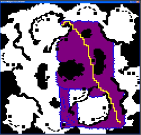
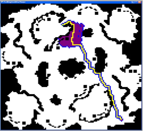
2 An example of an Weighted A* found path, showing the closed list . . . 6

3 A dead end highlighted in red on a 4-connected grid graph . . . 14

4 A dead end chain highlighted in red on a 4-connected grid graph . . . 15

5 A concave region . . . 18

6 A Simple Search . . . 21

7 Examples of Well-Formed Regions . . . 21

8 Examples of not Well-Formed Regions . . . 22

9 A region with a single boundary point . . . 24

10 A region with two boundary points . . . 24

11 A region with N boundary points . . . 26

12 A region with a single boundary . . . 26

13 A region with two boundaries . . . 27

14 A region with N boundaries . . . 27

15 A Transit Region . . . 29

16 An Axis Aligned Region . . . 31

17 Partition of Warcraft 3’s Battleground map . . . 33

18 Waypoint path . . . 35

19 A 4-connected unit cost grid graph . . . 37

20 A map from Baldur’s Gate . . . 37

21 Average Nodes Expanded on Warcraft 3 maps . . . 40

22 Average Nodes Expanded on Baldur’s Gate maps . . . 41

23 Comparison of A* against Transit Search on Warcraft 3 maps . . . 41

24 Comparison of A* against Transit Search on Baldur’s Gate maps . . . 42

(10)

List of Algorithms

1 A* . . . 5

2 Weighted A* . . . 8

3 Region Weighted A* . . . 13

4 Naive Maximum Allowed Heuristic Preparation . . . 19

5 Maximum Allowed Heurisitic Search . . . 20

6 Quad Tree Region Partitioning . . . 32

7 Transit Region Search Preparation . . . 33

8 Transit Region Search . . . 34

(11)

List of Symbols

G

A graph composed of nodes and edges

c(a,b)

The actual cost of the shortest path between nodes a and b

γ

A goal node for a search problem

s

The start node of a search problem

h(a,b)

A heuristic estimate of the shortest path’s cost between nodes a and b

g(a,b)

The minimum cost path from nodes a to b at the current point in the search

h(n)

A heuristic estimate of the shortest path cost from n to the goal state

g(n)

The minimum cost path from the start node to the node n at the current point in the

search

f(n)

The f-score of the A* algorithm; the value that is to be minimized

Pa,b

(12)

O(f)

The worst case computational complexity of the functionf

Υ

(13)

1 Introduction

1.1 Problem Domain

The problem of pathfinding is finding a path between two nodes in a graph. If we leta and b

be nodes in the graphG, a path is defined as a series of nodes starting with aand ending with

bsuch that each successive node is connected to the previous. Often we are concerned not with any path, but specifically paths which are of the least cost. The cost of a path is usually defined

as the sum of the weights along path.

Pathfinding has many uses in practical situations. Often real world data is converted into a

graph and searched to find shortest routes. Pathfinding is used extensively in video games to

plan the path that agents take. The game world is usually discretized into a graph with the

nodes being locations agents can travel to and the edges of the graph being the paths between

them. The weights on the edges are either cost of travel or distance between the nodes in the

search space. The pathfinding used in video games needs to be fast to allow for other systems

in the game to have enough time to run. Pathfinding also finds use in robotics and simulations

for planning the routes an agent may take.

More abstractly problems that involve searching can be solved with pathfinding algorithms.

Puzzles like the 15-puzzle can represent its configurations as nodes and and edges as the allowed

moves between them. This allows us to search for the smallest set of moves from a start

config-uration towards a goal one. It can also be used to find solutions to NP-Hard problems such as

the Travelling Salesmen problem.

1.2 Thesis

This thesis introduces a series of new algorithms that attempt to expand less nodes than A* (a

well-known search algorthm) does. The research culminates in the development of the Transit

(14)

algorithms. These will show that Transit Search is on average faster than A* and is comparable

(15)

2 Background

2.1 A*

The A* algorithm [HNR68] is a pathfinding algorithm that uses heuristic information to guide its

search toward a goal. It is an improvement over Djikstra’s algorithm [Dij59] in that it is informed

about the search space by means of an heuristic function. This function is used to measure the

expected cost to reach a goal node. A* is used to search within non-negative weighted graphs

composed of nodes and edges, from a start node s to a goal node γ. That is, it solves the

single-source shortest path problem on these graphs. A* is complete, in that if a path between

s and γ exists A* will find it. The algorithm always finds a least cost path, that is, no other

path has a lower cost. If there are multiple paths that have the least cost, A* will return one of

them.

Figure 1: An example of an A* found path, showing the closed list

(16)

2. h(n) This is the heuristic estimate of the cost fromnto a goalγ

Thus the f-score calculation looks like

f(n) =g(n) +h(n) (1)

This is contrast to Djikstra’s algorithm which essentially only considersg(n) and in contrast

to a greedy algorithm that would only take into accounth(n). This takes into account equally

the cost incurred so far and the expected cost of the rest of the path. As we expand nodes we

always take the node with the lowest f-score. This represents what we believe to be the next

node on the shortest path to the goal.

It often happens that there are multiple nodes with the same f-score and these are referred

to as the fringe. This is the set of nodes that A* could expand next. The rule we use to choose

which node to expand on the fringe is called a tie breaking rule. Changing the tie-breaking rule

can have a drastic effect when searching through graphs that can have a large fringe, sometimes

speeding search up by an order of magnitude.

There are some restrictions on what the heuristic function can be to ensure that A* returns

the shortest path. The first of which is admissibility. We say a heuristic function is admissible

if it never overestimates the cost to reach the goal. More formally a heuristic is admissible if,

∀n∈G, h(n, γ)≤c(n, γ) (2)

Admissible heuristics are optimistic as they often return a value that is less than the actual cost

to the goal.

Another restriction usually put on the heuristic is that of consistency. We say a heuristic is

consistent if,

∀a, b∈G, h(a, γ)≤c(a, b) +h(b, γ) (3)

given that b is a successor of a. If a heuristic is consistent it ensures that A* does not need to

recheck nodes on the closed list. It also lets A* be optimal up to a tie breaking rule. This means

that A* will expand a subset of the nodes of any other equally informed search algorithm, if it

is given the correct tie-breaking rule. This is important to note as other search algorithms using

the same information as A*, could be rewritten as A* with a particular tie breaking rule.

The A* algorithm is still an active area of research, with many other pathfinding algorithms

being based on it, or being variants of it. Work has been done to produce algorithms that limit

the time A* uses such as TBA* [BBS09]. Other algorithms have dropped the shortest path

(17)

work in reducing the number of nodes expanded on specific search spaces, uniform grids being

popular, in algorithms like RSR.

Algorithm 1: A*

add start to open list;

while open isn’t empty do

min = find min in open;

if min is goal then

return success;

end

add min to closed list;

foreachn in neighbours of min do

if n is in closed list then

continue;

end

if n was already opened then

change f-score if better;

else

n’s g-score = min’s g-score + edge cost from min to n;

n’s h-score = h(n,goal);

n’s f-score = n’s g-score + n’s h-score;

n’s parent = min;

add n to the open list;

end

(18)

2.2 Weighted A*

The Weighted A* search algorithm [Pea84] extends A* by using a weight on the heuristic in order

to speed up searches. This makes a node’s f-score more dependent on the heuristic estimate to

the goal and less on the cost already incurred along the path. If we letbe the weight, a constant

positive real value, then we can define the calculation of the f-score as,

f(n) =g(n) +∗h(n) (4)

Depending on the value that we choose for , the resultant effect on the search can differ.

Choosing an value of 1 we see that the formula for the score collapses to that of A*’s

f-score calculation. In this case Weighted A* would perform identical to A*, and this shows that

Weighted A* is a generalization of the A* search search algorithm.

Figure 2: An example of an Weighted A* found path, showing the closed list

If we let the weight be less than one ( <1) than f-score will be more sensitive to the path’s

cost and less sensitive to the heuristic. Viewing∗h(n) as some second heuristic functionh0(n), we can examine the effect this has on the search. Assuming thath(n) is admissible, thenh0(n) is also admissible since it must be less than equal h(n), and in no way could overestimate the

actual path cost. Sinceh0(n) is admissible, values of <1 maintain the shortest path guarantee of A*.

Even though it maintains the shortest path, these values of epsilon change the way the

algorithm expands nodes. Since we lower the effect h(n) has on the f-score, we increase the

relative effect thatg(n) has. Thus our algorithm is more likely to expand nodes that have lower

(19)

being more conservative than a weight of 1. In fact if we let = 0 then the f-score equation doesn’t consider the heuristic function at all, and our algorithm will run like Dijkstra’s algorithm.

This extreme makes the search uniform and loses the benefit of heuristics. Given that <1 we

put less trust in the heuristic and diminish its effect. Since we try to choose our heuristic to be

a good estimator of remaining cost, this only decreases the effectiveness of the algorithm.

We can however choose to be greater than 1 for a different result. When we have >1

the heuristic function has more of an effect on the calculation of the f-score. This makes our

algorithm more likely to expand nodes that are seen closer to a goal, based on the heuristic.

This puts more trust in the heuristic function, and since the heuristic function is chosen to be a

good estimator of actual cost, we would expect our algorithm to perform better.

The downside to choosing >1 is the effect it has on the path found. If h(n) is admissible there is no guarantee thath0₍_n_{) is also admissible, since}

∗h(n)≥h(n) (5)

This voids the conditions of A* that ensures that it finds an optimal path. Thus for Weighted

A* the paths returned may not be optimal (although they can be), and we have to trade-off

between path quality and speed. It is known though that the cost of the paths returned by

Weighted A* can be no more thantimes the cost of the path with the least cost. A calculated

choice ofcan then be used to balance the need for speed against the bounded sub-optimality of the paths found.

The algorithm for Weighted A* is very similar to that of A*. The singular change is that we

(20)

Algorithm 2: Weighted A*

if min is goal then

return success;

end

continue;

end

else

n’s h-score =* h(n,goal);

n’s parent = min;

end

return failure;

2.3 RSR

Rectangular Symmetry Reduction or RSR [HBK11], is an algorithm that prunes nodes within

rectangles of uniform cost grid graph. It does this by exploiting the symmetry of obstacle-free

rectangles so that it can create a smaller graph composed of the rectangle perimeters. It stores

a link from every node in the original graph to the rectangle it is within, so it can tell when

searching whether or not a node is in the rectangle of the node being expanded. This requires a

preparation step to find the rectangles and create the new graph. It also requires extra memory

of the complexityO(n), where n is the number of nodes in the graph. In addition information

on the rectangles is saved, namely the dimensions of the rectangle, and this requires space

(21)

The search phase inserts nodes from the original graph into the new graph and searches

along the perimeter of the rectangles. In order to connect nodes from one side of a rectangle to

nodes on the other side, edges are created to the nodes on the other side using the rectangle’s

information. This is done during the search and because of the simplicity of rectangles, can be

done in O(1) time. The algorithm also applies some extra online pruning to remove evaluating

(22)

3 Transit Region Search

3.1 Motivation

We want a faster search algorithm so that we can perform more searches and allow more time

for other algorithms in the program to run. This is more and more important as applications

keep increasing the number of agents requiring the use of pathfinding. Also as games add more

complicated physics, graphics and other systems the amount of time available for pathfinding

systems to run decreases.

In a variety of problems we also have perfect information before we search. We have access

to the graph offline in the case of pathfinding problems with perfect information. However,

algorithms like A* do not make use of this information in most cases, failing to alter the heuristic

based on the underlying graph. This produces algorithms that are more general and less specific

to individual graphs, and as such are unable to utilize the specific graph information.

The two ways we use to speed up searches are,

1. Trade off optimal path length for less nodes expanded

2. Use a preparation step to gather more information about the search space

Weighted algorithms make use of the first way, in that they use weights to trade off between path

length and the amount of nodes expanded. Changing the weight allows for multiple different

trade offs to occur. The second way increases the heuristic information of the search, making

in more informed than A*. This allows it to better expand nodes based on the information

gathered during the preparation step.

3.2 Region Weighted A*

When examining maps in video games we notice that there are areas within the maps having

certain attributes. These can be the size and shape of obstacles in the area, the room layouts

of buildings, the size of open areas and many others. When the search space is translated into

a graph these features can be as well. We want to exploit these features to make our search

algorithms more informed so they can search faster. The problem is describing areas of the maps

as substructures within the produced graph. We let a Region be such a substructure and define

a Region as a set of the nodes in a graph.

Since different areas of the map may have different properties, we want to reflect this when

searching within the regions they correspond to. We can do this by letting A* change its

behaviour in different regions. We know from Weighted A* that we can alter the f-score so that

(23)

so that it is dependent on the region of the node being evaluated, we might be able to better

search within regions.

We introduce the Region Weighted A* algorithm to be an algorithm whose f-score is

depen-dent on regions. We let a(r),b(r) and c(r) be functions of a region that produce a weight and

we change f(n) to be,

f(n) =a(r(n))∗g(n) +b(r(n))∗h(n) +c(r(n)) (6)

where r(n) is a function that returns the region that n belongs to. Now this requires that r(n)

exists for every node n. To facilitate this our algorithm ensures that∀n∈G,∃Rs.t. n∈R. We

accomplish this by creating%, a set of regions that is a partition of G.

It should be noted that our new f-score can collapse back to Weighted A*. Lettinga(R) = 1,

b(R) =and c(R) = 0, we have

f(n) = 1∗g(n) +∗h(n) + 0 (7)

Similarly, since this is now the f-score of Weighted A* this can also collapse back into A* by

letting = 1. These collapses only occur if we apply these changes to all R. Only changing a

single region might have the effect of A* within the region, but any node outside of the region

will be evaluated not as expected, due to the change in relative magnitude of the f-scores.

These changes make it necessary to have the a(r),b(r) andc(r) functions developed so that they can be called during search. We do this by means of a preparation step to be run offline

on the search space before we do any searching. This step is responsible for partitioning the

graph into regions and creating ther(n) function in order to tie a node back to its region during

search. Furthermore we require that we find the weight functionsa(r),b(r) and c(r) such that

for each region we produce a triplet of weights(a,b,c) to be applied to the search while in that

(24)

number of nodes in the graph.

Without knowing how exactly the weights affect the search it can be difficult to choose

weights that improve performance. Since for each region there are three weights and changing

any weight can change the performance of the search, we have many combinations of weights to

consider. If we letv be the number of values we are considering for weights then we can choose

v3|%| (8)

different configurations. This number is large enough that we can’t simply search every case.

We can however search the cases to find a better set of weights. Since the algorithm can collapse

to Weighted A*, we can find anthat produces a good result in Weighted A*. By letting all our regions useand collapse to Weighted A*, we guarantee that our weights produce an algorithm

that is at least as good. Using this as a starting point, we can search for better weights, changing

our weights only when there is an improvement. This can be accomplished by a hill climbing

algorithm in order to search toward a optimal set of weights. To ensure that we find a good result

we can also implement a random restart mechanism to avoid getting stuck in local maxima.

It is not only necessary that we find good weights, we also must find good regions. Randomly

choosing%can easily result in a region set that is unrepresentative of the underlying areas in the

map. Thus, it is important that we choose regions that reflect the features of the search we wish

to exploit. One way to do this is manually by visual inspection. Features such as obstacle density

and likeness to a maze on a video game map are easy to inspect when viewing the map. Thus a

designer could manually choose regions based on these features with relative ease. However not

all features are so visually obvious, and a designer might not wish to repeat this procedure on

every game map. We can then turn to an algorithm to choose regions for us, such as clustering.

Clustering algorithms can take a set of data like the nodes of our graph, and produce clusters

of similar nodes. We can define a similarity function to relate to a feature and use this in the

clustering process. Then we can take the produced clusters and convert them into regions. This

way we can have an automated algorithm that runs in the preparation step and aside from the

(25)

Algorithm 3: Region Weighted A*

if min is goal then

return success;

end

continue;

end

region = get region containing n;

else

n’s g-score =a(region)* (min’s g-score + edge cost from min to n);

n’s h-score =b(region) * h(n,goal);

n’s f-score = n’s g-score + n’s h-score +c(region);

n’s parent = min;

end

(26)

node, whether or not its neighbours are the goal (before putting in on the open set). But let’s

try a solution that utilizes region weightings.

First, let D be a region that contains all dead ends. Next we let D0 be the complement of

D, such that it contains all nodes which are not dead ends. Since we want our algorithm to

function like weighted A*(or just A*) inD0, we can set its weights to that of Weighted A*. For convenience, we will represent weights in the form of a vector comprised of< a(n), b(n), d(n)>

and for Weighted A* this looks like<1, w,0>for some weight w.

Figure 3: A dead end highlighted in red on a 4-connected grid graph

With region weighted A* our f-score function for E becomes

f(E) =a(D)g(E) +b(D)h(E) +d(D) (10)

In the case whereE6=Gwe never want to expandE. We can ensure this by makingf(E) have

a greater f-score than any other node, this way it will always get chosen last for expansion. Let

w∞ be a number that is greater than any f-score could possibly be on our graph, then when

E6=G, we letf(E)≥w∞. We know that the heuristic estimate never overestimates the actual

distance between any two nodes (assuming the heuristic is admissible), and this is true for E

and the node connecting to it. Thus if h(E) is greater than the distance between E and its

connected node(C), thenE 6=γ. Given this, we have a condition we can use to help us obtain

f(E)> w∞, when E is the goal, given by

ifh(E, γ)> c(E, C) thenE6=γ (11)

We can rewrite the previous inequality in the form of

ifh(E, γ–c(E, C)>0 thenE6=γ (12)

Since we needf(E) to be larger thanw∞ in this case, we can multiply both sides byw∞. We

can do this without worry of inverting the sign since,w∞ is always positive. Then we have

w∞(h(E, γ)–c(E, C))>0 (13)

(27)

we can leta(E) = 1, and updatef(E) tog(E) +b(D)h(E) +d(D). Then we let

b(D)h(E) +d(D) =w∞(h(E, γ)–c(E, C)) (14)

b(D)h(E) +d(D) =w∞∗h(E, γ)−w∞∗c(E, C) (15)

From this we see that we can assign b(D) =w∞ andd(D) =−w∞∗c(E, C), giving us a final

weighting of

D=<1, w∞,−w∞∗c(E, C)> (16)

Now we can see how this region weighting functions, first let us assumeh(E, γ)> c(E, C). In

this case, adding the last two terms produces a positive result that is a multiple ofw∞and thus

makesf(E)≥w∞, effectively making nodes belonging to D the last nodes expanded. Otherwise,

h(E, γ)≤c(E, C), and the sum of the last two terms is either 0 or a negative multiple ofw∞.

Since all other f-scores are positive the negativew∞ will always be chosen first to be expanded.

In a non-monotone distance case, it is possible we expand this node falsely, ifγis within the

heuristic distance but not equal toE. When that sum is 0, the f-score becomes the g-score, and

E will be expanded as soon as all nodes withf(n)< g(S, E) have been expanded. This ensures

that E is only ever expanded when γ=E, or all other nodes have been expanded. The latter

case would only occur if no such path exists, sincef(E) has a greater f-score than all other nodes

not inD and ifγwas inD, it would have a negative f-score and be expanded beforeE.

3.3.2 Dead End Chain

We define a dead end chain as a series of nodes starting with a dead end node, followed by a

sequence of nodes having 2 edges. The chain ends on the last node with 2 edges, and the non

chain node connected to this, is part of the rest of the search space. Let E be a dead end chain

withE0 being the dead end, andER−1 being the last node in the chain, whereR is the length

(28)

use of A*. We can calculate the distance fromE0 toE2 from using the distance fromE0 toE1

andE1 toE2 byd(E0, E2) =d(E0, E1) +d(E1, E2). This is true since to get toE2 fromE0 we

must travel through E1, by our definition of a chain. With this we can calculate the distance

betweenE0andE3byd(E0, E3) =d(E0, E2) +d(E2, E3). Generalizing this we have

d(E0, Ek) =

k−1

X

i=0

c(i, i+ 1) (17)

This gives us a formula to calculate the distance from the dead end to any other node in

the chain. This is important because it gives us a limit on how far we can travel towards the

dead end into the chain. We define a region for each node of a dead end chain (this can be

simplified to use less regions). We also let the weighting for the region not containing dead ends

be<1, w,0>, to emulate weighted A* not in dead end chains.

Considering the last node inE(ER−1), we never want our algorithm to expandER−1 unless

there is a chance the goal could be in E. If the goal isn’t inE there is no point in expanding

any of it, since E doesn’t lead to any other node. We know from above that we can calculate

the maximum distance one could travel into the dead end chain. Since the heuristic never

overestimates the distance, if it is greater than the max distance in the chain, there is no chance

that γ is inE. Thus if h(ER−1, γ)> c(E0, ER−1) +c(ER−1, C) then E is not in γ. Following

similar steps to the dead end formulation above we can obtain,

b(DR−1)h(ER−1) +d(DR−1) =w∞∗h(ER−1, γ)−w∞∗(c(E0, ER−1) +c(ER−1, C)) (18)

Putting this in terms of weights we have

DR−1=<1, w∞,−w∞∗(c(E0, ER−1) +c(ER−1, C))> (19)

We happen to knowc(E0, ER−1) so we can write

DR−1=<1, w∞,−w∞∗

r−2

X

i=0

c(i, i+ 1) +c(ER−1, C)

!

> (20)

This acts much like the dead end case; if the heuristic is greater than the distance to the

dead end, the goal is not in E, and the sum of the last two terms will be a positive multiple of

w∞. Since w∞ is larger than any f-score, it will be expanded last, ensuring we never enter E

if theγ can’t possibly be inE. When the heuristic is less than or equal to the distance toE0,

thenER−1 is either a negative multiple of wor 0.

(29)

When f-score turns negative, it will be expanded before non-dead end chain nodes, but it is very

possible thatγ is not in E when this happens. Our weights only ensure we don’t search down

the chain if goal can’t possibly be on it, but the more distance the chain covers, the higher the

maximum heuristic distance allowed becomes. This in turn makes it become expanded more

often, leading our search into the chain. Now we could just apply this weighting to all the

regions associated with nodes in our chain, but it would cause our search to reachE0every time

it expandedER−1. Instead we can change our weighting to

Dk=<1, w∞,−w∞∗

k−1

X

i=0

c(i, i+ 1) +c(Ek, Ek+1)

!

> (21)

This way every time we evaluate the f-score of a node in E, we tighten the requirement to

continue down the chain. This reduces the chance we travel more than we have to in order to

discover that we have taken the wrong path. In addition it works exactly like DR−1. This lets

our Region Weighted A* avoid unnecessary dead ends and paths that lead to dead ends, saving

a lot of nodes in the process(depending on the search space).

It is known that A* expands the least nodes to find the shortest path for a given heuristic

than any other algorithm. Upon reflection, we can rewrite the our f-score asf(n) =g(n) +h0₍_n_),

where

h0(n) =w∞∗h(ER−1, γ)−w∞∗(c(E0, ER−1) +c(ER−1, C)) (22)

That is to sayh0(n) is a piecewise heuristic that changes based on the local node. So really we can achieve better results than A* with a heuristich(n) because we are simply transforming the

heuristic to one that better estimates the distance to the goal. We just do so in a fashion that

uses the original heuristic and regions to dictate the pieces of the function.

3.4 Maximum Allowed Heuristic

(30)

shorter path. Since the path fromS toAandB toγare invariant to the path change, then the combined path length will be shorter than the original path fromS toγ. This can’t be because

the originalS toγ path is the shortest, thus no shorter path betweenAandB exists.

We use this concept by lettingB =γ, and examining the path asS to AandAtoγ. Then

ifS toγis the shortest path, and Alies onS toγ, thenAtoγ onS toγmust be the shortest

path. Thus any shortest path that goes through A must contain a shortest path starting with

A. Any path follows edges between nodes and thus this path must start with an edge fromA. If

we take the set of shortest paths starting withA and ending with all other nodes in the graph,

we can partition this set into collections corresponding to which edge they leaveAfrom. If there

are multiple edges that lead to the shortest path between A and some other node, we randomly

choose a partitioned set.

Next we can transform these partitions from sets of paths to sets of lengths, each being the

path length of its path. Then each collection is a set of all possible distances one can travel

to arrive at a goal, while taking the shortest path. We note that for dead ends, we use the

maximum amount of distance we could travel in the dead end to help exclude them. If we were

expandingAand evaluating the node across an edge and we knew that we could only travel so

far through this edge, we could apply a similar behaviour. Thus we find the furthest we could

travel along an edge, and use that as a cutoff to compare the heuristic distance to.

Figure 5: A concave region like the one highlighted can be avoided in some searches when using a Maximum Allowed Heuristic

Given that we have a set of the shortest distances (being the only distances we would travel

on shortest paths) by choosing the maximum of these we can find the furthest we can travel

while staying a shortest path. So if we were to expandA, and we knew the heuristic distance to

the goal was greater than this value, then no path going through that edge leads to the shortest

path to the goal, so we need not expand that node. By saving this maximum allowed heuristic

(31)

3.4.2 MAH Search

This algorithm uses a simple preparation step to give edges an extra weight that contains the

maximum allowed heuristic (MAH) value. We simply do an A* search from every node to every

other node in the graph. After we find each path we let the MAH be

M AH(edge) =M ax(M AH(edge),length of the new path)

This populates every edge in the graph with a MAH value that we can use in the search portion

of the algorithm.

Algorithm 4: Naive Maximum Allowed Heuristic Preparation

foreachnode A in all nodes in graph do

foreachnode B in all nodes in graphdo

if A is B then

continue;

end

find shortest path between A and B;

if path is found then

length = length of the found path;

followedEdge = the edge from A to the rest of the path;

followedEdge’s MAH = maximum of followedEdge’s MAH and length;

end

The search portion is nearly identical to A*. The only thing we change is that before we

evaluate a node while expanding some node A, we do a check. The check compares the heuristic

(32)

Algorithm 5: Maximum Allowed Heurisitic Search

if min is goal then

return success;

end

if min’s h-score>maximum allowed heuristic for edge min to n then

continue;

end

continue;

end

else

n’s parent = min;

end

return failure;

3.4.3 Complexity

The preparation complexity is really the problem with this approach. Since we have to check

every node versus every other node the time complexity of the preparation step is O(E∗n2_),

whereEis the number of edges in the graph. This is only the case in the naive approach shown

in algorithm 4 though. Using an approach that utilizes the Floyd-Warshall algorithm it should

be possible to reduce the time complexity toO(n3_{). The added space complexity is 1 value per}

(33)

The time complexity during the search step is the same as A*. We already know the heuristic

distance from the node we are expanding to the goal and the MAH is an O(1) retrieval. It is

expected it to be faster on average though, due to the nodes we avoided expanding.

3.5 Transit Regions

What we really want to accomplish is to be able to exploit the substructures found within a

search space in order to speed up search. While Maximum Allowed Heuristic Search avoids dead

ends, it still exhaustively searches through regions that a more simple search algorithm could

search through fast. Take for instance an undirected grid graph where every grid cell is a node.

Then we connect nodes that are horizontally and vertically adjacent with a weighted edge of

cost 1.

Figure 6: A Simple Search

In this graph searching is trivial with a Manhattan heuristic since we can just expand nodes

with the minimum h-score. This search expandspnodes, where p is the length of the path to be

found. What transit region search does is make use of regions where we can search faster than

A* and use A* in regions we can’t.

(34)

properties.

1. ∀a, b∈R,∃Pa,b s.t. ∀x∈Pa,b ,x∈R

2. ∀b∈R,∃y∈adjacent(b)∧y /∈R =⇒ bis a mandatory boundary node

3. ∀b∈R,|adjacent(b)|< κ =⇒ bis a optional boundary node

4. A boundary node is either optional or mandatory.

5. A region is composed of internal nodes and boundary nodes.

6. LetB⊆R∧ ∀b∈B b is a boundary node∧ ∀α, β∈B,∃Pα,β s.t. ∀x∈Pα,β ,x∈B then

B is a boundary.

Hereκis the maximum amount of nodes any node may have adjacent to it.

These restrictions exclude many of the previous regions; including all unconnected regions.

An immediate consequence of well-formed regions is that when performing A*, if the start and

goal reside in the same region, we have no need to expand any node outside of region. Since the

shortest path is within the well-formed region, no nodes on the path are outside of the region

and need not be expanded.

Figure 8: Examples of regions that are not well-formed. There is not a shortest path between some nodes in the green region, and the blue region is disconnected disallowing some paths altogether

Our approach depends highly upon 2 things. First how the heuristic function performs within

the region. This is a measure of strictly local performance, and we will try to isolate regions

with better local performance. Secondly, we depend upon the boundaries of the region. Given

different types of boundaries we can make assumptions and exploit interesting properties. We

identify 4 different types of heuristic performance within a well-formed region, being

1. Heuristically Perfect

(a) ∀a, b∈Rlet h(a,b) = h*(a,b)

(35)

(c) h*(a,b) = c(a,b), the heuristic distance returned is the actual distance

2. Heuristically Great

(a) ∀a, b∈Rh(n,g) = h*(n,g)

(b) min h* always picks the right node to expand

(c) h*(a,b) is not equal to c(a,b), it can give the wrong distance

3. Normal – no special properties

4. Misleading - heuristic more than often leads you down the wrong path

The algorithms we are proposing make use of Heuristically Perfect regions. The combination

of the heuristic always choosing the correct node to expand, tied with being able to accurately

calculate g-score by knowing h-score, gives us some powerful properties to work with. Note that

there are algorithms that make use of the other types of heuristic performance, and that they

can help improve over A*. We only focus on Heuristically Perfect Regions, as they provide us

with the most information that we can use to our advantage.

As for boundaries we identify them by 2 features. The first is the number of boundaries on

the region, which we deal with as 1, 2 or N. These correspond to paths that travel through the

region as no choice, 1 choice and many choices, given that a path enters through a boundary.

The second is the boundary path type, which we divide into point boundaries or multi-point

boundaries. A point boundary is comprised of a single node, and multi-point boundary has more

than one node.

3.5.2 Heuristically Perfect Regions

We will now we go through the combinations of heuristically perfect regions and provide

algo-rithms for searching them in a faster manner than A*. The first of these has 1 point boundary.

(36)

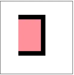
Figure 9: A region with a single boundary point

we know the distance to the goal. If we travel that distance down the path we should find the

goal. If we don’t then we know the goal isn’t in the region, and we can skip the rest of the nodes.

This means that we at most expand the number of nodes required to travel the MAH distance.

We also need only to store space for those MAH values for the boundary node, giving an extra

space complexity ofO(max edges of a node).

Next we discuss the Heuristically Perfect region with 2 point boundaries. Unlike the last

region this one can have a path that goes through the region, having a start and goal node

outside of the region. We can still make use of the maximum allowed heuristic to exclude nodes

within the region, but the max value would be a lot higher and very few nodes would be excluded.

Thus we use a local MAH; that is, we find the maximum distance one could travel within the

region through an edge. Similar to the global MAH previously employed, if our heuristic value is

greater than our MAH then the goal is further than any path in the region and much lie outside

of it. If this is the case, we can exclude the region, but the path could still be through the other

boundary, so we must expand it.

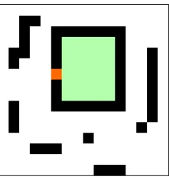
Figure 10: A region with two boundary points

The problem with expanding nodes not directly connected to the node we are expanding is

that we need to calculate its f-score. The heuristic distance to the goal isn’t a problem, but we

don’t know the actual distance from our expanding node to the other. However, remember our

(37)

f(J1) =g(J1, S) +h(J1, γ)

=g(J0, S) +g(J0, J1) +h(J1, γ)

=g(J0, S) +h(J0, J1) +h(J1, γ) (23)

This allows us to expand the other boundary from our boundary and know the exact f-score

of the node. This ensures an optimal path and allows us to skip over the other nodes in the

region, since we don’t need to travel them to discover the g-score forJ1. In the case where the

local MAH is greater than or equal to our heuristic, we have to search the region. Like the

previous case we can do this by doing a pure heuristic search, and only expand as far as the

heuristic distance.

Our node expansion is the same as the previous region, plus the expansion of the other

boundary. In terms of extra space needed its 2∗O(max edges of a node), as we need to store a

local MAH for every boundary edge that leads into the region. We also need a edge fromJ0 to

J1 to be added to the graph so we know to expand it (this isO(1)). We refer to this edge as a

bridge edge, as it is a bridge over the region. This is still a very small amount of space.

The third region we examine is the Heuristically Perfect region with N point boundaries.

This is similar to the previous case, except that we have more than one possible path exit when

a path travels through the region. If we find that we can skip the region, we have to open all

other exit nodes. This requires that we store a MAH value for every inner edge on a boundary

point. It also means we need to add a bridge edge from every boundary point to every other

boundary point. This increases the memory footprint to

O(|Υ| ∗max edges of a node) +O(|Υ| ∗(|Υ| −1)) (24)

(38)

Figure 11: A region with N boundary points

through a boundary point on the singular boundary, then there exists a path between the entry

and the exit that lies on the boundary which is shorter. Thus the path cannot be the shortest

path. This allows us to treat the boundary path like the single point boundary and avoid the

entire region based on the MAH of the boundary points, since no shortest path travels through

the region.

Figure 12: A region with a single boundary

There is more than one boundary point though and the extra memory is going reflect this.

We need to store a MAH value for every point on the boundary, so the extra memory amounts

to O(|Υ| ∗max edges of a node). We do not need to create any bridge edges since we don’t

travel through the region; if the path we are finding lies on the boundary, we just search with

normal A*. If we wanted to create bridges to speed up searches on the boundary it would be

approximately O(|Υ| ∗(|Υ| −3)) extra memory. This is a trade-off, but the extra memory cost

seems unwarranted for a small number of nodes not expanded.

We move onto a region that has a boundary composed of two paths. In this case we do have

to worry about paths that can travel through the region. This is like the N-Point boundaries

but we know a path that travels through the region must connect one boundary to another.

Thus if we can skip over a region based on the MAH, we need to open all nodes on the other

boundary. Then the number of edges we need to add amounts to |B1| ∗ |B2|, where B1 is the

(39)

our extra memory becomes,

O((|B1|+|B2|)∗max edges of a node +|B1| ∗ |B2|) (25)

We note that the number of nodes evaluated during expansion sharply increases on a boundary

node, but we hope to choose regions where we save even more node expansions by entirely

skipping the interior of the region.

Figure 13: A region with two boundaries

The final case we look at is where the boundary is composed of N paths. This is very similar

to the previous case. If a path travels through the region, it could exit through any boundary

that isn’t the one it entered. Thus we need to add bridge nodes from every node to every other

node not on the first nodes boundary. Thus we need to addP

i|Bi| ∗

P

j|Bj|bridge edges. This

increases our extra memory to

O(X

i

|Bi| ∗max edges of a node +

X

i

|Bi| ∗

X

j

|Bj|) (26)

We will be most concerned with this last case, as it is the most general and as such can be

(40)

single path boundary, consisting of a single point, with 0 interior nodes in the region. It is the

shortest path from itself to itself, so it meets the criteria of boundaries needing to be a shortest

path. Since a consistent heuristic never overestimates the path length to the goal, the heuristic

must return 0. If we make every node in the graph be its own region, those regions are N-path

heuristically perfect and it makes a partition of the graph.

This example is pretty much just to prove that we can partition any graph, it would be

useless for our purposes as the regions contain no interior nodes to skip. Ideally we want to

ensure that we have enough nodes to skip in order to justify the extra memory we are using.

Next we look into more requirements we could place onto these regions in order to reduce our

memory footprint.

3.5.3 Optimality

It is often stated that A* is an optimal algorithm, in that for some heuristic h(n) no other

shortest path algorithm will expand less nodes than A*. However the fact is this isn’t always

the case. First this only applies to algorithms that are as equally informed as A*. This means

that both algorithms are given the same heuristic information.

With our algorithms we use a preparation step to define regions where h∗(n) =h(n), and we use this information to change how we expand nodes. A* on the other hand does not have

access to this information. Therefore it is possible for our algorithm to expand less nodes than

A* while maintaining the shortest path because it utilizes extra information that A* does not.

Another interesting fact is that A* is not always optimal compared to another algorithm even

if they are equally informed. Decther and Pearl [DP85] showed that there are different types

of optimality and that A*’s type of optimality differs based on the class of the other algorithm

as well as the domain of the problem instance. In the class of algorithms that are admissible if

h(n)≤h∗(n) and the common problem domain of consistent heuristics, A* is only 1-optimal.

This means there exists a tie breaking rule that will expand a subset of nodes of any other

admissible algorithm. However because it is not 0-optimal, not all tie breaking rules will expand

a subset. This reflects the creation of tie breaking rules that perform better on certain problems,

as there is known to be at least one that will let A* outperform all other equally informed

(41)

3.5.4 Transit Regions

We define a Transit Region as an N-path Heuristically Perfect region that for every boundary

nodeJ there exists a boundary nodeK on every other boundary such that

g(J, Ki)≥g(J, K) +g(K, Ki) (27)

We callK a transit node ofJ. It should be noted that this is the reverse triangle inequality.

Figure 15: A Transit region showing a boundary node in blue, and its transit nodes on the other boundaries in gray

This makes it possible to greatly reduce the number of bridge edges we need for each boundary

node. Since the shortest path distance from J to someKi is always greater than or equal to the distance fromJ toK and thenK toKi, we can always take the latter path and be assured it’s

the shortest. Then we only need a bridge from J toK, and we can simply search the shortest

path fromK toKi, which is along K’s boundary path.

The memory requirement for an algorithm that uses Transit regions is also reduced. Since we

only need a single bridge from a boundary node to each other boundary, the number of bridges

becomes (|Υ| −1)∗P

i|Bi|, where|Υ|is the number of boundaries. The extra memory we use is

O(|Υ| ∗max edges of a node + (X

i

|Bi| −1)∗ |Υ|) (28)

(42)

3.5.5 Manhattan Distance

While all the previous algorithms will work on any non-negative weighted graph, we depart

to work on graphs where the heuristic used is a Manhattan one. This is fairly common in a

lot of search problems, and is often used in games. We seek to find a condition that makes a

Heuristically Perfect Region be a Transit Region, with the Manhattan Heuristic. We find these

for a general n dimensional Manhattan heuristic,

h(x, y) =X

i

(|xi–yi|) (29)

We know that on a transit region, our shortest path distance must satisfy

g(J, Ki)>=g(J, K) +g(K, Ki) (30)

And on an heuristically perfect regionh∗=h=g so we have,

X

j

(|Jj–Kij|)>=X

j

(|Jj–Kj|) +X

j

(|Kj–Kij|) (31)

We search for a coordinate wise solution, one that holds this condition for each j

|Jj–Kij|>=|Jj–Kj|+|Kj–Kij| (32)

There is however a triangle inequality for real numbers and absolute values that states

|a–c|<=|a−b|+|b–c| (33)

Thus we are left with a singular equality that must hold

|Jj–Kij|=|Jj–Kj|+|Kj–Kij| (34)

We note thatKj is chosen forJj and thus can be any node on the boundary K. Let us divide the problem into 2 cases.

1. Jj falls outside of the interval fromKj toKij

(a) IfJj is closer to Kj, thenJj and Kij form the end points of a line, and Jj–Kj+

Kj–Kij=Jj–Kij.

(b) IfJj is closer toKij, then this does not hold, but if we make the closestKij be Kj,

(43)

2. Jj falls inside the interval fromKj toKij a. This doesn’t hold unless Jj=Kj, otherwise the line formed hasJ as point on the interior of the line, and the distance some of the end

points + the end point andJ is always greater than the sum ofJ and the other end point.

When they are equal though, J becomes an endpoint and the Jj–Kj term becomes 0.

Thus we have conditions for our equation to hold, and when the equation holds, the

heuris-tically perfect region is a transit region.

If we use a Manhattan heuristic in a heuristically perfect region, then the region is a transit

region if for every boundary nodeJ, the projection ofJ onto the ith axis either

1. Lies outside of the interval created by projecting every other boundary K onto the ith

axis.

2. Lies exactly on the projection of some node k on every other boundary K onto the ith

axis.

This gives us a test to determine whether we can use our Transit Region algorithm on a region

or not.

3.5.6 Axis Aligned Regions

Getting even more specific we can make use of the previous proof in a case that occurs frequently.

Let us prove that on a grid space, using a Manhattan heuristic any heuristically perfect axis

(44)

The y coordinate then must project to the same node or not exist in the interval. Since

the boundaries are axis aligned only one of the coordinates will be within the interval, or the

boundaries overlap at node J. This ensures that the conditions are met for a transit region.

Therefore choosing our regions to be heuristically perfect axis aligned regions lets us also use

them as transit regions.

3.5.7 Implementation

Our implementation uses transit regions and it consists of a preparation step to partition the

search space into convex polygons(we opt to use rectangles for ease of use) and populate the

local MAH values of boundary nodes. Then online we search making use of the properties of

Perfect Transit Regions to avoid searching the interior of regions.

The preparation step uses a quad tree [?] based system to partition the graph into rectangular

regions. We set the root of the quad tree to represent the entire search space. Then if we find an

obstacle in the quad tree we split it into 4 children. We repeat this until two sets of tree remain,

those with only obstacles, and those without. We take the former to be our set of regions. Then

we do a combining phase where we join adjacent regions, to clean up regions that were split

poorly due to the where the quad tree chose to split.

Algorithm 6: Quad Tree Region Partitioning

currentTrees = a empty list of QuadTrees;

add a tree covering the entire search space to currentTrees;

while currentTrees isn’t empty do

nextTrees = a empty list of QuadTrees;

foreachQuadTree tree in currentTrees do

if tree contains no obstacles then

add tree to returnList;

end

else

split tree into 4 QuadTrees;

add these to nextTrees;

end

currentTrees = nextTrees;

end

return returnList;

(45)

Figure 17: The Warcraft 3 ”Battleground” map partitioned using the quad tree partitioning algorithm

only need to add a single bridge edge per node per other boundary, since the regions are Transit

Regions. We also don’t add bridges between adjacent edges since in a rectangle the shortest path

between adjacent sides can be found by following the boundaries using a Manhattan heuristic.

This means we are only adding 1 bridge per boundary node. After this we calculate the heuristic

distance of every path coming from an edge of a boundary node to determine the MAH value.

Normally one would have to do an A* search to obtain the path length, but since h(n) = h*(n)

= g(n), we can calculate it without having to do any searching.

Algorithm 7: Transit Region Search Preparation

regions = QuadTreeRegionPartitioning();

foreachregion in regions do

bounds = a list of the region’s bounds;

foreachbound in bounds do

foreachboundNode in bound do

boundNode’s MAH = maximum distance you can travel in the region’s interior

from boundNode;

(46)

bridge nodes. Next we check if the heuristic value is less than the MAH value. If it is, then

we need to evaluate every neighbour, if it isn’t, we don’t need to evaluate any neighbour that

is in the interior of the region. We still need to evaluate other neighbours that are boundary

nodes though. We add nodes that are interior nodes that we skipped to an ignored list, so that

we can keep track of nodes we have expanded and then closed versus nodes that we never even

considered.

Algorithm 8: Transit Region Search

if min is goal then

return success;

end

if min is a boundary node then

foreachboundaryNode connected to min by a transit edge do

EvaluateNode(boundaryNode);

end

if min’s h-score≤min’s MAH value then

call Evaluate Node on every neighbour of min that isn’t on the skippedList;

end

else

call Evaluate Node on neighbour’s of min that are boundary nodes add the

nodes that aren’t to the ignoredList;

end

else

call Evaluate Node on every neighbour of min, including those on the ignoredList;

end

(47)

Algorithm 9: Evaluate Node

return;

end

else

n’s parent = min;

end

There are some differences in the program output when compared to A*. When Transit

Search returns the path it can be reconstructed like A* from following each node’s parent. Unlike

A* however, the parents can be waypoints (boundary nodes on regions) and to get the actual

path you still need to reconstruct the path in between them. This is fast sinceh*(n) =g(n) in

a Transit Region and the resulting search can be done inO(p) time, where p is the length of the

path between waypoints. It should also be noted that we need not rebuild the path at all if

1. All we need is the path length, since the goal’s g-score gives this.

2. The underlying system’s agents can travel between waypoints.

The second case is common in video games as the pathfinding is employed to find a path that a

computer controlled agent can follow. The more points in the path to follow just increases the

work of agent moving. Since the agent could travel through an open area, like a transit region,

(48)

Another possible difference from A* is the quality of paths returned. Transit Search will

tend to return paths that axis aligned. Since we use axis aligned rectangles for regions, the

boundaries are vertical and horizontal lines. Many of the waypoints found on the path will

be on the boundary nodes and transit search can expand along the boundaries, producing axis

aligned lines. We view path quality as not one of the algorithm’s goals but it should be noted

that the paths returned have a tendency to be rectilinear. If the path quality wanted is more

diagonal, solutions like string pulling can always be run as a post process to improve the quality,

and this can be done inO(p) time.

3.6 Weighted Transit Search

A* can be changed to Weighted A* by adding a weight to improve performance but lose some

path optimality. Similarly we can apply this weighted approach to Transit search in order trade

optimality for speed. The change is near identical to that applied to A* in that we simply

transformh(n) toh0(n) where

h0(n) =∗h(n) (35)

One thing to note is that we still needh(n) when checking against the maximum allowed heuristic value. If we were to useh0₍_n_{) we could end up skipping over the region with the goal in it because}

(49)

4 Experimental Setup

4.1 Search Spaces

We choose to do our experiments on unit cost grid graphs. These are graphs in which the nodes

are cells on a grid connected to adjacent cells. We connect nodes if they are adjacent, and for

our purposes adjacency is defined as the cells above, below, right and left of a node. Each of

the edges has monotone weight of 1. This type of graph is used often in video games due to its

simplicity and ability to be a discretization of continuous search spaces.

Figure 19: A 4-connected unit cost grid graph

We picked search spaces from video games in industry namely, Warcraft 3 and Baldur’s Gate.

These were obtained from Nathan Sturtevant’s Pathfinding benchmarks freely available online

[Stu12]. The maps used are on a grid graph and connect their nodes with at most 4 edges

as previously described. These maps are used in practice and as such provide a good testing

environment for our algorithms. Our implementation of Transit Search exploits the sub-structure

of rectangles, and the maps used have a variety of larger areas and enclosed regions that can be

(50)

4.2 Assumptions

1. The search algorithms have perfect information. That is, the graph is known before the

search and more information is not discovered during the search. This is in fact needed

for Transit Search given its dependence on a preparation step.

2. The graph is static. Some problem instances are dynamic where the configuration of the

graph changes. We do not test on any of these instances. The preparation step creates

regions based on the input graph, any changes to the graph could invalidate the transit

regions.

3. All searches performed are between a single start node and single goal node. While we

could have a goal containing multiple nodes and a heuristic that accounts for this; we use

the simple case. This is common in pathfinding research.

4. The graphs are connected. This means there is a path from any node to any other, or

more concise

∀a, b∈G∃Pa,b (36)

5. The search spaces tested are representative of those used in a practical setting. We choose

maps from industry for this very purpose. We make the assumption that these maps are

a good representation of search spaces in other games as well.

6. All searches use the same tie breaking rule. In our implementations of the algorithms we

simply use the minimum element of a PriorityQueue in Java SE 8. We make no attempt

to sort nodes on the fridge based on any explicit tie breaking rule.

4.3 Algorithms

In our experiments we test and compare 4 different algorithms.

1. A*

2. Weighted A*

3. Transit Search

4. Weighted Transit Search

We use A* as a baseline for comparison as it is the most used pathfinding algorithm. It finds

least cost paths so it gives us a way to measure how sub-optimal the path lengths returned by

(51)

most nodes. This lets us also compare how much faster the other algorithms are compared to

A*.

With regards to the two Weighted algorithms, we choose two different weights to reflect

alternate uses of weights. We let = 1.1 to represent the cautious case as the path length

returned is bounded by 1.1 times the cost of the shortest path(1 in the case of our graphs). In

the other case we want to more reckless, not caring for how much longer the paths returned are,

we just want a faster search time. The weight we choose here is= 100.

Lastly we search using Transit Search. This maintains the shortest path like A* but skips

areas within the contour that A* must search. This should in most cases decrease the number of

nodes the algorithm needs to expand and we expect to see this in the results. In total we search

each path 6 times, twice for the weighted algorithms and once each for the others.

In all cases we use the Manhattan Heuristic defined as

h(a, b) =|ax−bx|+|ay−by| (37)

4.4 Paths Tested

The paths tested are chose at random from the graphs. We randomly choose a start node and

a goal node, then find the path between them. We know the path exists from our assumptions,

so we don’t need to worry about the path not being found. We reject a path outright if the

chosen start node and goal node are the same. This is done as the path length is 0 and all are

algorithms will exit on their first iteration with this result. No useful information can be gained

from that path, so we skip any of these paths.

Each map we test we choose 100 paths. Each of the six algorithms is run over every path so

that we can compare results on each data point. With the Warcraft 3 maps this gives us 1200

such data points and with the Baldur’s Gate maps we have 7400 more. This gives us a combined

(52)

A*, so we would expect them to do so.

Figure 21: Average Nodes Expanded on Warcraft 3 maps

Weighted A* using a weight of = 1.1 was the next most node expanding algorithm. It

expanded 4460 nodes and 5589 nodes respectively. This amounts to a speed increases of 1.67

and 1.43 times that of A*. Weighted A* is known to expand less nodes than A* and the results

confirm this, even with a weight only 10% higher than that of A*’s implicit weight of 1. When

we use a weight of= 100, the number of nodes expanded shrinks to 1658 and and 2213 nodes.

This is even more of an advantage, increasing speeds by a factor of 4.49 and 3.6 respectively.

Again, this is an expected result as the higher the weight we use, we care less about the increased

path length returned, and more about the speed of the algorithm.

Next we examine the results of the Transit Search algorithms that we have developed.

Tran-sit Search manages to expand 2764 nodes for Warcraft 3 maps and 3464 nodes for Baldur’s Gate

maps. This is an improvement in speed by 2.69 times and 2.3 times over that of A*. This shows

what we had hoped to prove, that Transit Search expands less nodes than A* and by a

consid-erable margin. Compared to Weighted A*, Transit Search also performs well. It outperforms

the algorithm when the weight is = 1.1, this is exceptional considering that Transit Search

maintains the shortest path, while Weighted A* loses its optimality to increase its speed. We

note that when the weight is higher though, at= 100, Transit Search does not outperform the

weighted search. It should be considered though that with the increase in weight, comes and

increase in the path lengths found.

We also tested Weighted Transit Search, which we expect to be faster than Transit Search,

but lose path optimality. This happens to be the case, with a weight of = 1.1, Weighted

Transit Search expands 1625 nodes and 2341 nodes. This outperforms all the previously tested

(53)

Figure 22: Average Nodes Expanded on Baldur’s Gate maps

If we increase the weight to = 100, the algorithm expands even less nodes at 719 and 1012

noes respectively. This is an improvement over all the other algorithms, running 10.3 and 7.87

Transit Search

University of Windsor

University of Windsor

Scholarship at UWindsor

Scholarship at UWindsor

Electronic Theses and Dissertations

Theses, Dissertations, and Major Papers

2014

Transit Search

Transit Search

Justin Moore

Transit Search

by

Justin Moore

Author’s Declaration of Orignality

Abstract

Acknowledgements

Table of Contents

List of Figures

List of Algorithms

List of Symbols

1

Introduction

1.1

Problem Domain

1.2

Thesis

2

Background

2.1

A*

2.2

Weighted A*

2.3

RSR

3

Transit Region Search

3.1

Motivation

3.2

Region Weighted A*

3.4

Maximum Allowed Heuristic

3.5

Transit Regions

3.6

Weighted Transit Search

4

Experimental Setup

4.1

Search Spaces

4.2

Assumptions

4.3

Algorithms

4.4

Paths Tested