CUI, HANYU. Extending Data Prefetching to Cope with Context Switch Misses. (Under the direction of Dr. Suleyman Sair).
Among the various costs of a context switch, its impact on the performance of L2 caches is the most significant because of the resulting high miss penalty. To mitigate the impact of context switches, several OS approaches have been proposed to reduce the number of context switches. Nevertheless, frequent context switches are inevitable in certain cases and result in severe L2 cache performance degradation. Moreover, traditional prefetching techniques are ineffective in the face of context switches as their prediction tables are also subject to loss of content during a context switch.
by Hanyu Cui
A dissertation submitted to the Graduate Faculty of North Carolina State University
in partial fullfillment of the requirements for the Degree of
Doctor of Philosophy
Computer Engineering
Raleigh, North Carolina
2009
APPROVED BY:
Dr. Edward Gehringer Dr. Eric Rotenberg
Dr. Suleyman Sair Dr. Yan Solihin
DEDICATION
BIOGRAPHY
ACKNOWLEDGMENTS
Firstly, I would like to thank my parents, who love me, teach me and always believe in me. No matter what happens, they are always encouraging and supporting me.
I would also like to express my gratitude to my advisor, Dr. Suleyman Sair. I could not have completed my dissertation without his guidance. And he always encouraged me when I had difficulties. Besides research, he also shared with me his experience on pursuing a career and adapting to the U.S. society as an international student.
My gratitude also goes to my advisory committee, for their invaluable feedback and suggestions on my dissertation and research. And I am very grateful for their help on my job searching, without which I could not have received my current offer under in such a economy.
I want to take this opportunity to say ”thank you” to my girlfriend. She has been always encouraging and supporting me. And she never hesitated to spend the time to help me out when I was on tight deadlines with my research, dissertation and interviews. We have been in perfect harmony ever since we met. I am so lucky to have her with me along the way.
I am also very thankful to the people in Center for Efficient Scalable and Reliable Computer (CESR), for the inspiring conversations we had and the help they offered countless times.
TABLE OF CONTENTS
LIST OF TABLES . . . vii
LIST OF FIGURES . . . viii
1 Introduction . . . 1
2 Related Work . . . 6
2.1 Context Switches . . . 7
2.1.1 Studies of Context Switches . . . 7
2.1.2 Reducing the Impact of Context Switches . . . 9
2.2 Prefetching Schemes . . . 10
2.3 Shared Cache Management . . . 12
2.4 Memory Bandwidth . . . 14
2.5 Phase Analysis . . . 15
3 GHL Prefetching . . . 18
3.1 Case Study . . . 19
3.2 Architecture Overview . . . 19
3.3 Prefetch Placement Policy . . . 23
3.4 Operations . . . 24
3.5 Feedback Mechanism . . . 26
3.6 CMP Extension . . . 28
3.7 GHL-NLP Hybrid Scheme . . . 29
3.8 Phase-Guided Prefetching . . . 29
4 Methodology . . . 34
4.1 Overview . . . 35
4.2 CMP Extension . . . 35
4.3 Context Switch Emulation . . . 37
4.4 Selecting Simulation Point . . . 38
4.4.1 Introduction . . . 38
4.4.2 SimPoint . . . 39
4.4.3 Variable-Length Phases . . . 40
4.4.3.1 Classifying Basic Blocks . . . 42
4.4.3.2 Tracking Basic Block Reuse with an LRU Stack . . . 43
4.4.3.3 Interval Generation . . . 46
4.4.3.4 Hierarchical Clustering . . . 50
5 Evaluation . . . 55
5.1 Evaluation of GHL-Prefetching . . . 56
5.1.1 Evaluation on Uni-Processors . . . 56
5.1.2 Evaluation on CMPs . . . 65
5.2 Comparison with Other Schemes . . . 71
5.3 Evaluation of Phase Guided-Prefetching . . . 89
6 Conclusions. . . 94
LIST OF TABLES
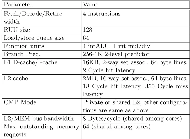
Table 4.1 Architectural configuration. . . 36
Table 4.2 Simulation parameters. . . 36
Table 5.1 Baseline bandwidth utilization. . . 74
LIST OF FIGURES
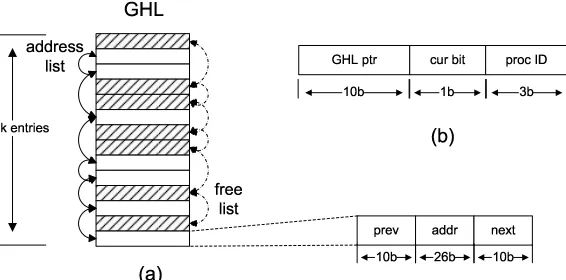
Figure 3.1 Context switch trace collected with SystemTap. . . 20 Figure 3.2 (a) The Global History List, shown here with 1K entries. Blank entries are
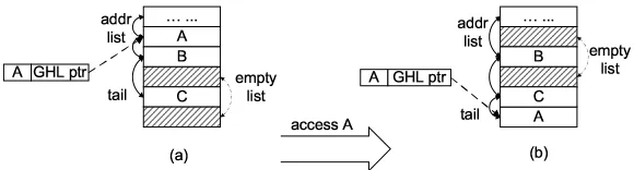
containing valid block address and linked together to form the address list. Shaded entries are unused entries and form the free list. As shown in the bottom, each GHL entry has three fields. Prev and next point to the previous and next entry in its own list respectively. (b) Additional information kept in each cache line. “GHL ptr” is a 10-bit pointer pointing to the corresponding GHL entry. “cur bit” indicates whether the cache is brought in by the current process. “proc ID” indicates by which process the block is brought in. . . 20 Figure 3.3 Removing duplicates in the GHL. (a) The three entries closest to the tail
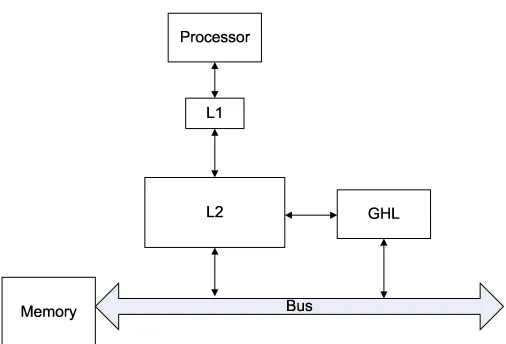
of the address list contain C, B and A respectively. The GHL pointer in the cache line that contains block A is pointing (the dashed line) to the corresponding entry in the address list. (b) After an access to block A, the old entry that contains A is reclaimed (becomes shaded) and a new entry is allocated for A at the tail of the address list. The GHL pointer then points to the new entry. . . 22 Figure 3.4 Location of GHL. Block ‘GHL’ represents all components related to GHL
except those in the L2 cache. . . 23 Figure 3.5 (a) Mapping between the reuse bit array and the address list, e.g. position 0
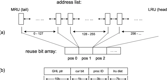
in the reuse bit array corresponds to entry 0 through 127 in the address list. (b) In addition to the fields in Figure 3.2 (b), a “lru dist” field is added to each line, which contains the corresponding position in the reuse bit array. . . 27 Figure 3.6 (a) Phase table. (b) Markov table. (c) Phase prediction. Prediction is made
at the beginning of sample interval yand tables are updated at the end. . . 31
Figure 4.1 The big picture. . . 42 Figure 4.2 Example illustrating how the LRU stack is updated. . . 45 Figure 4.3 Example illustrating how the LRU stack is used to form segments. Basic
are shown in the second row. The third row are the LRU stack hit depth of the basic blocks. Segments have already been generated following the rules above. Two different segments are separated by a space. . . 47 Figure 4.4 Merging segments into intervals using an LRU stack. . . 48 Figure 4.5 Calculating Manhattan Distance between segments/intervals. . . 51 Figure 4.6 Hierarchical clustering example in a two dimensional space. Each point
represents an interval. Each oval indicates a cluster where a pair of intervals are merged in every iteration. The number on an oval is the iteration number in which the clusters were merged. . . 53
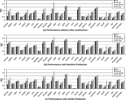
Figure 5.1 Performance with and without GHL-prefetching. Four cases are compared in each graph: context switch is present (sw), context switch with GHL-prefetching ( sw-pf), context switch with GHL-prefetching and feedback (sw-pf-fb), no context switch ( no-sw). . . 58 Figure 5.2 Used and unused GHL-prefetches. Two cases (sw-pf and sw-pf-fb) are
pre-sented for each benchmark. The y-axis shows the percentage relative to the number of GHL-prefetches without feedback (sw-pf), i.e. prefetching with feedback issues fewer prefetches. . . 59 Figure 5.3 (a) Percentage memory traffic increased in the presence of different
prefetch-ing schemes. Results are presented for GHL-prefetchprefetch-ing only (none), with a NLP (nextline) and with a Stride prefetcher (stride). For each of these cases, results with and with-out feedback are shown. (b) Performance with different context switch intervals. (b) Performance with different GHL sizes. . . 60 Figure 5.4 Performance when varying the number of outstanding memory requests
al-lowed. Sw shows the average IPC without any prefetching schemes while sw-pf-fb
shows the any IPC of GHL-prefetching. . . 61 Figure 5.5 Context switch misses remaining with our prefetching scheme using various
size GHLs. . . 63 Figure 5.6 (a) Performance with different interfering benchmarks. (b) Percentage of the
original application’s blocks that survive a context switch under various interfering benchmarks. . . 64 Figure 5.7 GHL-prefetching interacts with non-GHL cores. No context switching on
Figure 5.8 GHL-prefetching interacts with non-GHL cores. There is context switching on all cores. Results for 4 combinations comb 0 - comb 3 are shown. There are 4 configurations for each benchmark: single, where each benchmark is run on a uni-processor;CMP-2Mp, where each group are run on a 4-core CMP with 2M private caches; CMP-2Ms, where each group are run on a 4-core CMP with a 2M shared cache;CMP-512Kp, where each group are run on a 4-core CMP with 512K private caches. . . 67 Figure 5.9 Speedup of 16 benchmarks grouped into 4 groups. 4 configurations are shown
for each benchmark: single, where each benchmark is run on a uni-processor; CMP-2Mp, where each group are run on a 4-core CMP with 2M private caches;CMP-2Ms, where each group are run on a 4-core CMP with a 2M shared cache; CMP-512Kp, where each group are run on a 4-core CMP with 512K private caches. . . 69 Figure 5.10 IPC of 16 benchmarks with GHL-prefetching grouped into 4 groups. 4
configurations are shown for each benchmark: single, where each benchmark is run on a uni-processor;CMP-2Mp, where each group are run on a 4-core CMP with 2M private caches; CMP-2Ms, where each group are run on a 4-core CMP with a 2M shared cache; CMP-512Kp, where each group are run on a 4-core CMP with 512K private caches. . . 70 Figure 5.11 IPC of 16 benchmarks with GHL-prefetching grouped into 4 groups. Number
of max outstanding memory requests is 128. 4 configurations are shown for each benchmark: single, where each benchmark is run on a uni-processor; CMP-2Mp, where each group are run on a 4-core CMP with 2M private caches; CMP-2Ms, where each group are run on a 4-core CMP with a 2M shared cache; CMP-512Kp, where each group are run on a 4-core CMP with 512K private caches. . . 71 Figure 5.12 (a) Speedup of GHL-prefetching (sw-pf-fb), Stride prefetcher (sw-stride) and
NLP (sw-nextline). (b) Memory bandwidth of the three prefetchers. (c) Efficiency of the three prefetchers. . . 73 Figure 5.13 (a) Average speedup when increasing the prefetching degree of a Stride
prefetcher. (b) Average speedup when increasing the table size of a Stride prefetcher. (c) Average speedup when increasing the prefetching degree of NLP. . . 75 Figure 5.14 Average CAMR sizes with 500K instruction intervals. . . 77 Figure 5.15 Percentage of misses that are with in 4 blocks from the end of a CAMR. . . 78 Figure 5.16 Coverage of GHL-prefetching (sw-pf-fb), NLP (sw-nextline) and Stride prefetcher
(sw-stride). Misses are broken down into 4 types: eliminated context switch misses
(cntxmiss), eliminated normal misses (miss), residual context switch misses (
Figure 5.17 Prefetch timeliness of GHL-prefetching (sw-pf-fb), NLP (sw-nextline) and Stride prefetcher (sw-stride). Prefetches are broken down into 4 types: prefetch hits (hit), delayed prefetch hits (delayed-hit), replaced prefetches (replaced), and mis-prefetches (miss). . . 81 Figure 5.18 Comparing GHL-prefetching (sw-pf-fb), NLP (sw-nextline) and the
GHL-NLP hybrid scheme (ghl+nextline): (a) Speedup. (b) Prefetch efficiency. . . 82 Figure 5.19 Average speedup across all benchmarks for GHL-prefetching (sw-pf-fb) and
saving tags (tag*). The blocks show the speedup while the line shows the percentage of memory bandwidth increase. . . 83 Figure 5.20 Compares GHL-prefetching (sw-pf-fb) to Stride prefetcher (sw-stride) and
Stride prefetcher with saving its tables across context switches (sw-stride-save): (a) Increased IPC. (b) Increased bandwidth. (c) Efficiency of the three schemes. 84 Figure 5.21 Performance of our GHL-prefetching mechanism with a 2MB L2 cache
com-pared to the performance of larger caches. . . 85 Figure 5.22 Comparing average (a) IPC and (b) Speedup of GHL-prefetching (sw-pf-fb),
NLP (sw-nextline) and Stride (sw-stride), each with 4 different configurations: uni-processor (single), private 2M L2 caches (CMP-2Mp), shared 2M L2 (CMP-2Ms), and private 512K L2 caches (CMP-512Kp). . . 86 Figure 5.23 Comparing the 3 prefetchers with 2M private L2 caches. (a) Speedup of
GHL-prefetching (sw-pf-fb), NLP (sw-nextline) and Stride (sw-stride). (b) Prefetch efficiency of the 3 prefetchers. . . 87 Figure 5.24 Comparing the 3 prefetchers with 2M shared L2 cache. (a) Speedup of
GHL-prefetching (sw-pf-fb), NLP (sw-nextline) and Stride (sw-stride). (b) Prefetch efficiency of the 3 prefetchers. . . 88 Figure 5.25 Accuracy of phase predictor. . . 91 Figure 5.26 (a) Speedup of GHL-prefetching (sw-pf-fb), GHL-phase hybrid approach
with 50k and 200k sample intervals (sw-hybrid-50k and sw-hybrid-200k), Stride prefetcher (sw-stride) and NLP (sw-nextline). (b) Prefetching efficiency of the two approaches . . . 91 Figure 5.27 (a) Average speedup when increasing prefetching degree of Stride prefetcher.
Chapter 1
Most time-shared operating systems use context switching since it leads to faster response times, higher throughput and fairness as well as higher utilization of system re-sources. However, context switches hurt cache performance as cache state belonging to different programs compete for cache space and replace each other’s lines. Since most of these interfering programs do not share any data or instructions, the cache content built up by the swapped out process is of no use to the new process. The new one would have to bring all its data and instructions into the cache all the way from memory and results in many cold misses. We call these missescontext switch misses. Given the speed gap between memory and on chip caches, this creates a significant bottleneck.
Because context switches are so expensive, various techniques have been proposed to reduce their impact. Most operating systems (OS) are designed to minimize the number of context switches whenever possible. For instance, the minimum quantum for a process is 5 ms in Linux Kernel 2.6 [4], which makes context switches rare enough to have small overhead in many cases. Alternatively, affinity scheduling [34, 55] also helps reduce the number of context switches by giving higher priority to the currently running process. While this gives the current process a better chance of retaining the processor, it hurts the responsiveness and fairness [1] of the system. Cache partitioning is another solution to prevent processes from clobbering each other’s state [53]. However, this reduces the usable cache space for each process. Furthermore, if the number of processes exceed the number of available partitions, even the partitioned cache will suffer from context switches.
next sequential block should be prefetched. A stride prefetcher [7] captures access patterns that have a fixed stride. Markov prefetchers [23] try to discover global correlation between addresses. Solihin et al. [52] proposed using a User-Level Memory Thread (ULMT) for correlation prefetching, which takes advantage of cheap memory and software’s flexibility. However, the prefetchers mentioned above do not specifically target context switch misses. Nesbit et al. [39, 40] use the Global History Buffer (GHB) for holding the most recent miss addresses in FIFO order for subsequent prefetching. Their approach is close to our scheme, but with different goals. They are also different in several aspects, which are discussed in section 2.
In this work, we propose eliminating context switch misses via prefetching to miti-gate the impact of context switches. Prefetching is advantageous over previously mentioned schemes: (1) Prefetching frees the OS to focus on other scheduling criteria (responsiveness, fairness etc.) by removing restrictions such as minimum time quantum limits or increased the priority of the current thread; (2) In cases where frequent context switches are inevitable, e.g. in the presence of network streaming, multimedia processing or inter-process piping, OS based techniques do not perform well; (3) Cache partitioning is fundamentally geared towards a different problem (resolving conflicts among simultaneously running threads in a CMP) and is ineffective when there are more threads than partitions.
which rely on arithmetic patterns in address streams, our technique can capture irregular accesses. And unlike common context-based prefetchers (e.g. Markov [23]) which are limited by predictor table size and are themselves subject to loss of content during context switches, our technique stores the contents of the prefetcher along with the program state so that it can be restored upon being swapped in.
Given the size of caches and program’s working set nowadays, our scheme needs to prefetch a large number of memory blocks following a context switch, which could potentially consume too much memory bandwidth and thus offset its benefits. Based on our design mentioned above, we come up with two schemes that aim at improving accuracy of the prefetcher. The first one is a feedback mechanism that tracks which prefetches are used and make predictions for future prefetch uses accordingly. Only the blocks that are predicted to be used will be prefetched. The second one is a phase-guided prefetching scheme, which captures the unique phase behavior certain benchmarks have. These two schemes effectively eliminate a significant number of useless prefetches, improving performance while preserving precious memory bandwidth.
prefetcher with or without saving tables across context switches, and saving tags of the L2; and (9) attaining 36% average speedup over no prefetching, and 11% and 24% average speedup in the presence of other prefetchers.
Chapter 2
In this chapter, we present research done in context switches and its impact on system performance, which demonstrates the need to cope with L2 cache context switch misses. We discuss various OS studies and scheduling techniques related to the costs associ-ated with context switches. We also compare our design to various relassoci-ated prefetching and cache management schemes. Research done in phase analysis is discussed and compared to our phase-guided prefetching scheme. Furthermore, we discuss potential bandwidth con-sumption of our scheme.
2.1
Context Switches
2.1.1 Studies of Context Switches
Context switching is an indispensable component of modern operating system. However, it also comes at a cost. In this section, we are going to present prior research in the impact of context switches.
To estimate the effect of a context switch on cache performance, Mogul et al. [37] obtained address traces from a multi-tasking system, marked them with context switch information and fed them through a cache simulator. They showed that the overhead of a context switch can be up to hundreds of microseconds or thousands of cycles. On modern processors and OSs, this amounts to hundreds of thousands of cycles.
Liu et al. [31] studied the impact of context switches on cache misses. They characterized previously-unreported cache misses caused by context switches, which they call reordered misses. They are different from the commonly known context switch misses (they call them replaced misses), which are caused by one program’s working set being replaced by another program’s between two context switches. Reordered misses are not caused by displacement of cache blocks, rather, the blocks’ recency was changed by another program’s working set and thus has a higher chance to be replaced by the originally-running program when it is swapped in. In this dissertation, we adopt the commonly known “context switch miss” which is equivalent to their replaced miss. They also proposed an analytical cache model that accurately predicts context switch misses.
Fromm et al. [15] showed that the impact of context switches on L1 caches is insignificant. While they mentioned reducing the impact of context switches via duplicating caches or prefetching, they did not investigate them. In any case, duplicating the caches (or the tag arrays to guide prefetching) only addresses the issue of context switches among two processes. It would not be helpful in a more heavily loaded system.
Tsafrir [56] showed periodic hardware interrupts have a non-negligible overhead. It should also be noticed that interrupt handlers usually do not perform much work, but they may wake up a sleeping process which could preempt the current one. And since hardware interrupts are asynchronous, the operating system or user has no control over the number or frequency of the interrupts. Large numbers of or frequent interrupts could lead to frequent context switches and thus degrade system performance.
on mechanisms to mitigate such impact.
2.1.2 Reducing the Impact of Context Switches
Since context switching has significant impact on lower level cache, various schemes have been proposed to mitigate it.
Suh et al. [53] established an analytical cache model for a time-shared system and proposed cache partitioning to eliminate context switch misses. Compared with partition-ing, our scheme utilizes cache more efficiently because at any moment, the running process always has the entire cache to itself instead of a small partition. Furthermore, partitioning is ineffective when there are more processes than the number of partitions or the size of a partition becomes too small to be useful.
A processor with fast context switches enabled [2, 16, 26, 50, 54] can store the contexts of multiple threads/processes in hardware. It mitigates the impact of long latency operations by context-switching to another thread/process that is ready to execute. Since its context switches happen at instruction granularity, multiple threads are actually competing for the shared caches simultaneously. This is very similar to the threads running on a CMP. In contrast, our research focuses on threads/processes time-sharing the processor, which complements their studies.
the same processor. Temporal affinity scheduling can be applied to context switches in a uniprocessor. However, its effectiveness would be reduced in heavily loaded systems because delaying scheduling other processes in favor of the one with temporal affinity could result in significant performance degradation, for example, due to lost packets. In general, our approach provides the OS the scheduling flexibility to address the needs of the current workload.
2.2
Prefetching Schemes
Our approach is to use prefetching to eliminate context switch misses. There have been many related prefetching schemes in the literature.
An early example of a prefetching architecture is Nextline Prefetching (NLP) by Smith [51], where each cache block was tagged with a bit indicating a prefetch should be issued. Using this bit, when a prefetched block is accessed by the program, a prefetch of the next sequential block is triggered. This scheme is simple yet effective, especially for programs with sequential access patterns.
A stride prefetcher [7] keeps track of the difference between the last address of a load and the address before that, which is called the stride. The prefetcher speculates that the new address seen by the load will be the sum of the last address value and the stride. This type of prefetcher is very effective for programs with regular array accesses, e.g. scientific program that perform matrix manipulations.
by the same set of misses.
Kandiraju et al. [24] proposed distance prefetching by generalizing Markov prefetch-ing. It was originally proposed for TLB prefetching and later on turned out to be also effective for data cache prefetching. It has the same idea as Markov prefetching, which is to capture the global correlation between addresses and use similar tables to store prefetcher states. Different from Markov prefetching, instead of capturing the correlation between actual addresses, it tries to capture the correlation between the distances of successive ad-dresses. The distances, instead of the actual addresses, are stored in the prefetcher tables. If a distance x is predicted, a prefetch is issued with a target computed by adding x to the current address. (or previously issued prefetch if the prefetcher goes further down the correlation chain) Using the distances enables more compact tables and can potentially cover more addresses. However, it could also have more aliasing since the distance space is smaller than the address space by far.
Solihin et al. [52] proposed using a User-Level Memory Thread (ULMT) for corre-lation prefetching. It needs a general purpose processor at the memory side, with minimal changes to the main processor and other architectural components. Since it is closer to the main memory, it can prefetch farther ahead with shorter latency. Since it is using a software thread, it is more customizable than a pure hardware scheme. They also proposed an improved correlation prefetching scheme that exploits that fact that memory is cheap and the prefetcher is closer to the memory.
cooperative software-hardware prefetcher [30]. In this scheme, the compiler inserts prefetch hints for load instructions and the region prefetcher would issue the prefetches in hardware. The above prefetching schemes are usually effective for the type of misses they are targeting. However, none of them specifically target context switch misses. On the other hand, context switch misses are special in that they are not inherent to the program, but they are also significantly affected by hardware, how frequently context switches take place, and what programs are run between context switches. These factors make the mentioned schemes unsuitable to cope with context switch misses. Moreover, none of them save any state in the main memory and thus are subject to meta data loss across context switches.
Nesbit et al. [39, 40] proposed the Global History Buffer (GHB) for holding the most recent miss addresses in FIFO order for subsequent prefetching. The GHB has two advantages over traditional predictor tables: it eliminates stale prediction data, and it maintains a complete picture of cache miss history. The GHB is similar to our approach in that both are trying to record the global history. However, they have three fundamental distinctions: (1) The GHB only records misses while our scheme records all read accesses; (2) Our scheme tries to remove duplicates and compact the history while the GHB does not because doing so would break how it operates; (3) We save the access history along with the state of the process while it is being swapped out so that it can later be restored. As a result, our scheme is more suited to warming up cache state after a context switch.
2.3
Shared Cache Management
happen if the number of processes is more than the number of physical cores, which make the two schemes complementary.
Qureshi and Patt [43] proposed utility-based cache partitioning (UCP), which partitions a shared cache among multiple applications depending on how many misses could potentially be reduced for a given amount of cache resources. It achieves higher throughput than LRU replacement policy because it partitions resources based on whether the resource is going to bring the highest return, not whether the requesting application has the highest demand. They also design an efficient mechanism that monitors all running applications and make partition decisions.
Kim [25] et al. studied the fairness in cache sharing among multiple threads in a CMP environment in detail. Their work complements prior research on cache sharing, which only focuses on characterization and optimization techniques on throughput. They proposed several metrics that measure fairness and cache partitioning algorithms that improves fair-ness. They also studied the relation between fairness and throughput and indicate that increasing fairness usually result in improved throughput while the opposite is not always true.
alternating the biggest partition among multiple threads, every thread has the chance to progress as fast as possible instead of being slowed down constantly by a small partition.
Guo [17] et al. proposed a frame work to provide quality of service (QoS) to applications on CMPs based on shared cache management. They proposed a way to specify QoS targets, as well as an admission policy that accepts jobs according to their QoS targets. They found that enforcing a strict QoS target has significant impact on system performance because of resource fragmentation and proposed a mechanism that solves this problem by “stealing” excess resources from some applications.
All of the above schemes only focus on sharing caches among threads that are executing simultaneously but none of them studied threads time-sharing the processor(s). Our research complements them by studying threads/processes time-sharing the processor, and by using prefetching instead of partitioning the shared cache.
2.4
Memory Bandwidth
There has been extensive research on techniques and architectures that enhance performance of the memory bus and DRAM memory in the literature [19, 35, 36, 45, 57]. Since our scheme needs to prefetch a large number of memory blocks into the processor, high speed bus and memory architectures can boost its performance in some cases.
bank. They proposed several scheduling policies and attained close to peak bandwidth via aggressive reordering. Since our scheme needs to prefetch many blocks right after a process is swapped in, it would be advantageous to implement our scheme on a system with memory scheduling. By scheduling prefetches issued by GHL according to the memory architecture, higher bandwidth and smaller delay can be expected. Our design simply give higher priority to demand misses but does not perform any memory scheduling. This could be one of our future directions.
2.5
Phase Analysis
In this section, we are going to discuss prior research in phase analysis, which is related to our phase-guided prefetching scheme in section 3.8.
In order to guide dynamic cache reconfiguration for energy conservation, Bala-subramonian et al. [3] proposed collecting hardware counters to observe miss rate, CPI and branch frequency information for every 100K instructions. Their algorithm used these hardware counter values to determine if a reconfiguration needs to be triggered because of a drastic change in program behavior. Similarly, Isci and Martonosi [21, 22] observed that a program’s power consumption can exhibit phase behavior. They proposed using power vectors to identify this behavior. Duesterwald et al. also observed periodic phase behavior across multiple metrics measured with hardware performance counters [14]. They introduced cross-metric predictors that use one metric to predict another, thus enabling an efficient coupling of multiple predictors.
instruction the working set. They then employ these changes in program working sets for initiating instruction cache, data cache and branch predictor reconfiguration [9, 10].
Sherwood et al. [47, 48] showed that periodic phase behavior in programs can be automatically identified by profiling the code executed. For this purpose, they proposed associating a Basic Block Vector (BBV) to each fixed length execution interval. BBVs are one dimensional arrays where each element in the array corresponds to one static basic block in the program. The execution starts with a BBV containing all zeroes at the beginning of each interval. During each interval, for each basic block that is executed, they increment the corresponding vector element by the number of instructions in the basic block. This ensures that blocks containing more instructions will have more weight in the BBV. In a nutshell, a BBV can be considered as the fingerprint for the interval it was collected for. Subsequently, thek-means clustering algorithm [33] is used over all the BBVs to group intervals of execution that were alike into the same phase. The authors observed that phases formed in this manner exhibited similar behavior across a variety of architectural metrics. Based on this analysis, they presented the SimPoint toolset that identifies a small set of representative simulation points for detailed architectural simulation. They also extended this approach to perform hardware phase classification and prediction [49].
Another means of extracting phase behavior was proposed by Huang et al. [20]. They examined tracking procedure calls via a call stack, which can be used to dynamically identify phase changes. More recently they proposed using procedure call boundaries for creating samples to guide statistical simulation [32].
They analyze the data reuse distance trace. They analyze the data reuse distance trace, which is analogous to our LRU-stack based technique described in Section 4.4.3.2.
Lau et al. analyze the program behavior over a hierarchy of interval lengths [27]. This framework is built on top of the SimPoint toolset and uses the same basic block vectors. Two changes to SimPoint were needed to support their work. The first was the explosion in the number of intervals that needed to be analyzed due to the need to experiment with a hierarchy of interval lengths. They addressed this issue by randomly sampling intervals and performing clustering on those. The second change was supporting non-uniform weights in theirk-means clustering algorithm. They also presented initial results using SimPoint and Sequitur with variable length intervals for creating a hierarchy of variable length intervals. Both of these techniques use the Sequitur string matching algorithm to identify hierarchical phase behavior.
We extend Sherwood et al. [49]’s work to capture data access phases by calculating signatures with a new algorithm from data accesses and tuning all parameters accordingly. By utilizing phase analysis and prediction, prefetching is more accurate. Combing phase-guided prefetching with GHL-prefetching yields higher speedup.
Chapter 3
In this chapter, we present the details of ourGHL-prefetchingarchitecture and the motivating forces behind its design.
3.1
Case Study
As mentioned in Section 1, frequent context switches are inevitable in certain cases. We used SystemTap [44] to collect the context switch trace from a real machine. The machine is a single core Pentium 4 3.0 GHz machine running Linux Kernel 2.6.17. Part of the collected trace is shown in Figure 3.1. Each entry of the trace has three fields: a sequence number, process ID with the name of the executable, and the duration (in µs) a process runs before being swapped out.
The case shown here is typical. The user is running two tasks. One application is scp copying a large file to another computer. The other is cc1, which is invoked by gcc to compile some code. We can see that it is actually sshd that does the actual work while copying files over an ssh tunnel. The trace shows that sshd and cc1 interrupt each other frequently. Most of the time, they can run no more than 600 µs before a context switch occurs. The average runtime without context switches forcc1 is approximately 300
µs and 100 µs for sshd, which translate into 900K and 300K cycles for a 3GHz machine respectively. Our experiments show that such frequent context switches have a significant impact on the performance of the L2 cache and the entire system.
3.2
Architecture Overview
01 3071(scp): 6(us) | 17 3096(cc1): 2192(us) 02 2440(upsd): 17(us) | 18 2440(upsd): 19(us) 03 3096(cc1): 509(us) | 19 3096(cc1): 133(us) 04 3069(sshd): 23(us) | 20 3069(sshd): 23(us) 05 3096(cc1): 103(us) | 21 3096(cc1): 73(us) 06 3069(sshd): 18(us) | 22 3069(sshd): 17(us) 07 3096(cc1): 98(us) | 23 3096(cc1): 128(us) 08 3069(sshd): 18(us) | 24 3069(sshd): 16(us) 09 3096(cc1): 112(us) | 25 3096(cc1): 102(us) 10 3069(sshd): 17(us) | 26 3069(sshd): 16(us) 11 3096(cc1): 100(us) | 27 3096(cc1): 113(us) 12 3069(sshd): 18(us) | 28 3069(sshd): 17(us) 13 3096(cc1): 138(us) | 29 3096(cc1): 123(us) 14 3069(sshd): 550(us) | 30 3069(sshd): 559(us) 15 3071(scp): 75(us) | 31 3071(scp): 77(us) 16 3069(sshd): 6(us) |
Figure 3.1: Context switch trace collected with SystemTap.
! "#" $%
"#&
'
! $%
"(&
)* +-,* )* ./ 02143
56-*
7598:
)* * ;*
information kept in each cache line. The prefetch buffer is just a FIFO that stores the addresses to be prefetched and the rest of the components will be explained in detail.
The GHL is a buffer organized into two doubly-linked lists: the Address List and
the Free List, which are shown in Figure 3.2 (a). Each GHL entry has three fields: an L2
cache physical block address and two pointers. The pointers point to the previous entry and next entry respectively, either in the address list or the free list. The address list records all L2 read accesses, while the free list holds the unused entries. To record an L2 access, one entry is taken from the free list and inserted at the tail of the address list. To reclaim an entry, we remove it from the address list and insert it back into the free list. The pointers in the affected entries are changed accordingly in these operations.
The address list is maintained in LRU order meaning new block addresses are inserted at the tail. We record the accesses on a per-process basis. When the process is swapped out, the block addresses in the address list are saved in a dedicated region in main memory. The next time this process is swapped in, the block addresses (physical) will be loaded into the GHL and the prefetch buffer to guide prefetching. Prefetches are issued starting from the MRU entry to bring in the most recently used data items into the L2 cache first.
!
"
#
!
"
#
Figure 3.3: Removing duplicates in the GHL. (a) The three entries closest to the tail of the address list contain C, B and A respectively. The GHL pointer in the cache line that contains block A is pointing (the dashed line) to the corresponding entry in the address list. (b) After an access to block A, the old entry that contains A is reclaimed (becomes shaded) and a new entry is allocated for A at the tail of the address list. The GHL pointer then points to the new entry.
To reduce the on-chip area overhead, we adopt a two-level GHL scheme with a small on-chip component and a larger off-chip part. The GHL described above will be the
on-chip GHL, which caches the most recently accessed addresses. The off-chip part, referred
Figure 3.4: Location of GHL. Block ‘GHL’ represents all components related to GHL except those in the L2 cache.
3.3
Prefetch Placement Policy
Since thousands of blocks are being prefetched, it is very important to not replace useful blocks, which include two categories: (a) blocks brought during the current interval, including demand and prefetched blocks; (b) blocks brought in previously by the current process. The first category is referred to ascurrent blocksand the second category is referred to assurvivor blocks. Identifying survivor blocks from prior intervals requires distinguishing blocks brought in by all interfering processes. Since this requires tagging each cache line with a large process ID field but does not bring enough benefit, we chose not to implement survivor block identification.
The GHL and related components are not on the critical path. They only com-municate with the L2 cache and the main memory bus, as shown in Figure 3.4. Since most operations (in Section 3.4) related to GHL are only for performance and does not affect correctness, they can be delayed if necessary.
3.4
Operations
GHL-prefetching includes maintaining the access history during execution, saving the address list upon a context switch, and after being swapped in, loading the address list and issuing prefetches.
Recording accesses: Whenever there is an L2 read access, an entry is allocated
in the on-chip GHL and inserted at the tail of the address list. If this insertion results in duplication, the older entry will be removed as described in Section 3.2. Note that when a cache line is replaced, we do not reclaim the address list entry corresponding to the replaced line. Therefore, it is possible that an address is still in the on-chip GHL but the corresponding block has been replaced in the cache. In this case, the pointer to the on-chip GHL entry is lost and there is no way to reclaim that entry even if it is a duplicate. Our experiments show that this does not result in a noticeable waste of entries. When there is an L2 access but no entries in the free list, we move the oldest entry in the address list to the off-chip GHL. As we described in Section 3.2, the oldest entry in the off-chip GHL will be overwritten when it becomes full.
Saving the address list: When a process is swapped out, besides saving its context,
installed when the list is repopulated upon swapping the process in.
Loading the address list and issuing prefetches: When a process is swapped in
later, the addresses saved in the off-chip GHL will be loaded into the prefetch buffer to guide prefetching. Since the buffer has only 1K entries, prefetching will begin after it has been filled or all saved addresses have been loaded. A single prefetch is issued every cycle from the prefetch buffer. The next 1K will be loaded after prefetches have been issued for the current ones. The first 1K addresses will also be inserted at the head (LRU entry) of the address list of the on-chip GHL, until it becomes full. When a prefetch is issued for any of these 1K entries, the “GHL ptr” in the destination cache line is changed to point to this entry. This enables duplicate removal for the 1K MRU addresses. Unlike a demand access, issuing a prefetch does not move the entry to the tail of the address list. We consider the time it takes to save and repopulate the first 1K entries of the address list to be part of the context switch overhead. The latter parts of the off-chip GHL are brought in as bandwidth permits while the process is running.
prefetches physical memory blocks into the L2 cache. However, some types of memory pages are uncacheable and cannot be placed in the L2 cache. To make sure blocks in these pages are not prefetched, GHL records an access only if the accessed block can be placed in the L2 cache. This can be easily known at the time of the access. Another problem caused by uncacheable pages is that this attribute can be changed dynamically and blocks already in the caches and GHLs could become uncacheable. When this happens, the OS needs to flush the caches and the on-chip/off-chip GHLs. Since such changes are rare in real systems except in system initialization stage, they do not cause any noticeable performance degradation to GHL-prefetching.
3.5
Feedback Mechanism
We found that depending on the behavior of the program, the percentage of useful prefetches varies and sometimes is low enough to cause significant waste of memory band-width. Our experiments reveal that a certain cluster of prefetches would be used, followed by a series of wasteful prefetches. Furthermore, this pattern exhibits temporal locality across different executions of the same process. Hence, we use a reuse bit array to record which prefetched blocks are used by the program. Each position in this reuse bit array corresponds to a GHL entry allocated a certain number accesses ago (e.g. the LRU order). Since the address list is also in LRU order, the reuse bit array can be mapped to the entries in the address list and used to track which addresses in the address list are used by the program. If the access pattern of a program remains fairly stable across context switches, prefetching only the addresses that are used eliminates most of the useless prefetches. Our experiments show that this assumption holds for most of the benchmarks we studied.
"! #%$'&)()$+*-,.-/0##1/2'3
/-440#%$(5(76,(8.93
:
;
<
=
>
?
@
A
B
:
C
D
<
E
?
@
A
F
G
/'H
IJK-LMN OQPNRSM LNTOUV
R R WR
G
*H X
NPYZS[M
R
Figure 3.5: (a) Mapping between the reuse bit array and the address list, e.g. position 0 in the reuse bit array corresponds to entry 0 through 127 in the address list. (b) In addition to the fields in Figure 3.2 (b), a “lru dist” field is added to each line, which contains the corresponding position in the reuse bit array.
One issue with the feedback mechanism is that once we stop prefetching blocks in a certain address list region, we cannot detect whether they become useful in the future. Thus, we issue a prefetch for the first block in each region regardless of its reuse bit value. As a result, if the prefetched block is reused, the corresponding bit in the reuse bit array would be set and cause the entire region to be prefetched. This would result in a minor waste of memory bandwidth, but ensures that we do not ban a certain range in the address list forever.
3.6
CMP Extension
Our original scheme is designed for a uni-processor. In this section, we discuss how it can be applied on CMPs. GHL-related components can be duplicated with each core. Prefetch requests from multiple GHLs are treated on a First Come First Serve (FCFS) basis. No extra communication hardware is needed for GHLs on different cores.
the GHL and thus does not introduce extra delay. Further design of the circuity is out of the scope of this dissertation and will not be further discussed.
3.7
GHL-NLP Hybrid Scheme
Recognizing that GHL-prefetching and NLP are complementary, we designed a hybrid scheme that tries to take advantage of the strengths of both schemes by adaptively alternating between the two prefetchers. Since GHL-prefetching already has a feedback mechanism in place, we will use this feedback information to choose which scheme we will use after a context switch. When more than 50% of the bits of the reuse bit array are set (defined in Section 3.5), only GHL will be used for prefetching. When fewer than 50% of the bits are set, this is a good indication that GHL is not being effectively utilized. In this case, we activate NLP and not use GHL-prefetching. However, GHL-prefetching will continue to record accesses and one prefetch will still be issued for each region indicated by the reuse bit array, as mentioned in Section 3.5. Experiment results show that by taking advantage of the reuse bit array, the better prefetcher can be selected in most cases.
3.8
Phase-Guided Prefetching
change. Combining the two schemes will lead to higher performance.
The phase-detection techniques we adopt are based on those of Sherwood et al. [49]. A program’s execution is divided into intervals, referred to as the sample intervals. Two intervals sharing a large number of addresses are considered in the same phase. Signatures are computed from the accessed addresses in each interval. Signatures need to be compact and tell how many addresses two sample intervals share. We found that signatures that can accurately identify different phases require at least 512 bits. Different from Sherwood’s scheme [49], it is calculated through a combination of bitwise and modulus operations on load addresses. For each block addressX and a prime numberY close to 512, Xmodulo Y
locates a bit in the signature and this bit is set.
The signatures of all phases are saved in the phase-table in Figure 3.6 (a) and its position in the table is its phase ID. TheMarkov table in Figure 3.6 (b) saves possible phase transitions. Each entry has one phase ID and a “Next Phase” field, where the phase ID of possible transitions are saved, together with their confidence counters. The confidence counters are 2-bit saturating counters. Our simulations show saving 4 transitions are sufficient for each phase.
! "# %$'&( ) ( +* ,-". & ,/ " &/ * ,10 $
23/ 5476 89
: # *
; ; <>=?+@?
? <A@?
< B:;
B ?CD?>=<AE< F )
(1 G%HI J G H J < < J *I B H J <% H KL1
I I1K
Figure 3.6: (a) Phase table. (b) Markov table. (c) Phase prediction. Prediction is made at the beginning of sample interval yand tables are updated at the end.
table will be invalidated.
Phase classification is a time-consuming operation since a significant number of phase-table entries need to be searched before a phase can be determined. To speed up the operation, the signature of the predicted phase x will be compared first. If it is a hit (Manhattan distance below a certain threshold), no more entries need to be searched. If it is a miss, the remaining entries will be compared against the signature of interval x. However, it does not delay prefetching since prefetches are not issued in this case anyway (explained in the next paragraph). This is also how the previous prediction is verified. The corresponding confidence counter in the Markov table will be incremented if the previous phase was predicted correctly and reset if predicted incorrectly. Transitions with non-zero confidence counter values are deemedconfident transitions.
Prefetches are issued based on the prediction. Though a prediction is made at the beginning of each interval, not every prediction triggers prefetches. Only when (1) there have been at least three consecutive correct predictions and (2) the current prediction is a confident transition would prefetches be triggered. As a result, searching the phase-table does not delay prefetching because it only takes place when the last prediction is incorrect and no prefetches are issued in this case.
In order to obtain the L2 accesses for a certain phase, we take advantage of the on-chip GHL. Whenever the end of a sample interval has been reached, a special entry is inserted into the GHL to separate accesses between different phases. The accesses of the current phase will be saved to the a dedicated region in main memory if the transition is deemed confident. In our design, we allow at most 100K addresses to be saved in the main memory. Since memory is cheap, this is not too expensive.
GHL-prefetching and phase-guided prefetching work together to form a hybrid scheme. If phase-guided prefetching is triggered, GHL-prefetching will be delayed until it finishes. If a certain number of confident phase transitions have been predicted, no GHL-prefetches will be issued except for one per region indicated by the reuse bit array, which is mentioned in Section 3.5.
Chapter 4
4.1
Overview
Our simulator is based on the timing simulator in SimpleScalar 3.0 toolset [5] for the Alpha AXP ISA. Its configuration is shown in Table 4.1. We extended the baseline simulator to model queuing at the various levels of the memory hierarchy. However the detailed structure inside the main memory is not modeled. It is viewed as a whole and accesses to different rows or columns are not distinguished.
We evaluate our scheme on all benchmarks in the SPEC’2K benchmark suite. For each benchmark we use the reference input set and simulate a single simulation point ob-tained with SimPoint [18]. Each simulation alternates between the simulated benchmark and an interfering benchmark until the main application is executed for 500 million instruc-tions. Unless noted otherwise, the results presented in the next section are the average across all benchmarks and are collected with the parameters shown in Table 4.2.
4.2
CMP Extension
Table 4.1: Architectural configuration.
Parameter Value
Fetch/Decode/Retire width
4 instructions
RUU size 128
Load/store queue size 64
Function units 4 intALU, 1 int mul/div Branch Pred. 256-1K 2-level predictor
L1 D-cache/I-cache 16KB, 2-way set assoc., 64 byte lines, 2 Cycle hit latency
L2 cache 2MB, 16-way set assoc., 64 byte lines, 18 Cycle hit latency, 350 Cycle miss latency
CMP Mode Private or shared L2, other configura-tions are same as above
L2/MEM bus bandwidth 8 Bytes/cycle (shared among cores) Max outstanding memory
requests
64 (shared among cores)
Table 4.2: Simulation parameters.
Parameter Value
GHL size 16K entries, 1K on-chip, max 15K off-chip
Reuse bit array 128 entries Interfering benchmark art
Context switch period 1M cycles Interfering benchmark
du-ration
1M instructions
Nextline Prefetcher Prefetch degree is 4
on how they are used. For instance, a shared L2 cache needs to be protected by a mutex, which guarantees exclusive accesses. To ensure correct timing, there is a barrier at the end of each cycle that synchronizes all threads.
We examine both private and shared L2 cache schemes. The private L2 scheme manifests the bandwidth problem for a CMP machine but does not involve managing the shared caches, which was already studied extensively in literature [6, 25, 53]. The shared L2 scheme is more common in modern CMPs and shows interesting interaction among the cores. With either scheme, we focus on prefetching and no cache management mechanism is applied.
4.3
Context Switch Emulation
We used the SimpleScalar cache simulator with similar configuration to our timing simulator to collect L2 read access traces for several of the SPEC’2K benchmarks. We use these traces to emulate the effects of a context switch on the cache hierarchy. At each context switch, for each address in the trace, we clear the valid bit of the corresponding L2 cache line. Following a context switch, we assume the interfering benchmark runs for 1M instructions (only part of which are loads). After this, the main application resumes execution. Since we do not have a scheduler, we trigger context switches at a fixed period. We also tried random context switch intervals and found that there was not a noticeable difference as long as the mean of the random intervals was the same as the fixed period. This scheme consumes less simulation time than real execution and is accurate enough.
give similar results. However, they are different when applied on a CMP. This is because context switches could happen at different times on different cores. As a result, the inter-fering benchmark on one core could compete for resources with the interfered benchmarks on other cores. Using only traces is not able to simulate the correct timing and resource consumption. In both schemes, the triggering of context switches is the same.
4.4
Selecting Simulation Point
4.4.1 Introduction
Since architectural timing simulation takes a long time, researchers usually choose to simulate a small portion of the entire execution of a benchmark. They typically skip the initialization stage of the program and run timing simulation for a certain number of instructions. However, there is no guarantee that the selected portion would give the same, or even similar results as the full run. We need a more systematic methodology to approach this problem instead of blindly selecting the portions right after the initialization stage.
On the other hand, the large scale behavior of programs has been shown to be cyclic. As loops and function calls dominate program execution, the inherent repetition in these constructs culminate in this phase behavior. Recent research [3, 9, 10, 47, 48, 49, 42, 14, 28], has shown that it is possible to accurately identify and predict these phases in program execution. In addition, they have found that a few phases account for the majority of program execution. The top 20 phases account for 99% of execution for most SPEC programs [49].
tim-ing simulation [47, 48] without runntim-ing to the end. One or more portions of the full run, which belong to several major phases, could be selected to simulate. Since they belong to several major phases (phases that account for most of the execution), they are representative of the full run and can yield similar results.
4.4.2 SimPoint
SimPoint [18, 48] is a tool that can automatically classify analyze a program’s profile off-line and choose one or a few simulation points that can be representative of of the full run.
The entire execution of a program is divided into fixed length intervals. The length of the intervals could be from several million to hundreds of millions of dynamic instructions. It is a fixed-length approach because the length will be the same for all intervals once it has been chosen. SimPoint will try to classify these intervals into phases, and select on interval from each phase, which is the most representative of that phase.
After reading the input file, SimPoint performs k-means [33] clustering on the BBVs and similar BBVs will be grouped together and form a phase. Finally, one interval will be selected from each phase as a simulation point. This interval is the one with a BBV that is at the centroid of all BBVs in the phase (consider an n-element BBV is a point in an n dimension space). SimPoint also supports selecting a single simulation point, which greatly facilitates simulation, and keeps the error rate almost the same in most cases.
4.4.3 Variable-Length Phases
Most techniques that identify program phases, including SimPoint, first divide the execution into fixed-size contiguous intervals. In the next step, a footprint or signature of each interval is generated. Then they compare the signature of an interval to those of other intervals and group “similar” ones into a phase. Thus, intervals in the same phase can belong to different sections of execution (i.e. they are not necessarily temporally adjacent). One shortcoming of this approach is its reliance on fixed-sized intervals. If the beginning of an interval does not overlap with the actual phase change, we cannot identify the phase transition point accurately. Even worse, we create a slew of transitionary phases, whose intervals do not exhibit homogeneous behavior. That means optimizations such as resizing the cache for this phase can produce suboptimal results because theoretically this transitionary phase includes intervals of two different natural program phases.
phase behavior. We first start by profiling program basic blocks in terms of the instruction mix (e.g. number of integer ALU ops, number of branches etc.). Based on this profile, we group basic blocks that are similar in their composition into a single basic block type. We believe grouping in terms of instruction types is a more accurate approach in reducing the dimensionality of the basic block search space when compared to random projection as is customary in prior work. In addition, instead of using basic block vectors and string matching (described in more detail in Section 2), our approach relies on the reuse distance between program basic blocks to determine natural phase boundaries. And finally, rather than using thek-means clustering algorithm, we employ a hierarchical clustering algorithm that is more adept at finding similarities among intervals.
Variable-length interval generation is challenging. Relatively long intervals are required to make them representative of whole program execution and manageable for the clustering algorithms. However, even if the same section of code is executing, there are minor differences in the instruction stream due to control flow changes. And at the intersection of two repeated sections, there is usually “noise” which exhibits rather random behavior.
Basic Blocks Segments
Intervals Intervals Phases
…
Figure 4.1: The big picture.
Figure 4.1 shows all the steps we take to generate phases. We form segments from basic block. From segments, we form multiple levels of intervals. An interval in the higher level consists of one or more from the lower level. Finally, we perform hierarchical clustering on the highes level intervals to genearte phases.
4.4.3.1 Classifying Basic Blocks
proportional to the complexity of a phase classification mechanism, it is critical to reduce the number of dimensions. To efficiently track basic block execution and extract useful information from it, we need to reduce the dimensions to a manageable size (e.g. less than 16). Sherwood et al. perform random projection on the beginning PCs of basic blocks to reduce the dimensionality of the basic block space [47]. This approach has some shortcomings however. First, the PC of a basic block does not reveal any information other than its location in the memory. Secondly, random projection maps PCs randomly to a much smaller range without taking advantage of any information about the basic blocks. As a result, two basic blocks with completely different behavior could be mapped into the same dimension.
We address these issues by performingk-means clustering [33] on the basic blocks to classify them into the desired number of classes (16 in our case). We categorize the instruction stream into several classes (e.g. floating point, integer, load, branch, etc.). Then, we count the number of each different instruction class in every single basic block and form this into a vector where each dimension is an instruction class. Finally, we perform
k-means on the vectors to combine basic blocks with a similar composition into the same basic block type.
4.4.3.2 Tracking Basic Block Reuse with an LRU Stack
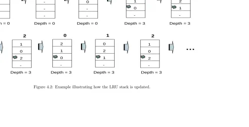
elements. When scanning the stream, we search every stack entry to find out whether the current element is in the stack. If not, it is a miss and the element is pushed onto the top of the stack. If the current element is found at the top, the stack hit distance is 1; if it is the second one from the top, the stack hit depth would be two, and so on. On a stack hit, the current element is moved to the top of the stack. As a result, a smaller stack hit depth indicates that an element reappears soon after its previous occurrence. An example is shown in Figure 4.2. The sequence is shown on the top and how the LRU stack generates hit depth is shown below it. We can see that, after the ”warm up” stage, the hit depth keeps to be 3, which means we have a loop consisting of three basic blocks.
To capture repeated execution of basic blocks, we use an LRU stack that is accessed with the type IDs of executed basic blocks. Each time a basic block is executed, we update the LRU stack with its basic block type ID. It’s the same thing we did in Figure 4.2 except that the original sequence is replaced by the sequence of type IDs. We follow the two rules below to merge basic blocks into segments:
1. Consecutive basic blocks with the same hit depth will be merged into a single segment.
-0
Depth = 0
0
-1
1 0
-2
2 1 0
-0
0 2 1
-1
1 0 2
-2
Sequence: 0 1 2 0 1 2 0 1 2 …
2 1 0
-0
0 2 1
-1
1 0 2
-2
Depth = 0 Depth = 0 Depth = 3 Depth = 3
Depth = 3 Depth = 3 Depth = 3 Depth = 3
…
following the rules above. Two different segments are separated by a space.
We use segment composition vectors to represent the resulting segments. The number of dimensions in a segment composition vector is the number of basic block types. Each dimension stores how many times the corresponding basic block executed, weighted with the basic block’s instruction count. The resulting segment vectors are shown in the lower right portion, which will be explained and used in next section.
We have two observations from the segments generated:
1. Our technique inevitably involves a “warm-up” problem. At the beginning of a new loop, there are always several misses when the stack is cold and thus the first iteration of a loop will always be separated the rest. This will generate more short segments than necessary. We tried to combine it with the rest but found that would result in a lot of false hit and involved tedious and complex algorithms. According to our experiment results, this ”warm-up” problem didn’t have a noticable impact on the number of intervals generated.
2. The two loops result in quite different segment patterns. The first loop only results in two segments, the first iteration of which is the result of a ”cold” LRU stack. The second loop results in a lot of short segments, which is caused by the alternating stack hit depth. However, by applying LRU stack recursively, which is shown later, most of these short segments will be merged together due to their repeated pattern.
4.4.3.3 Interval Generation
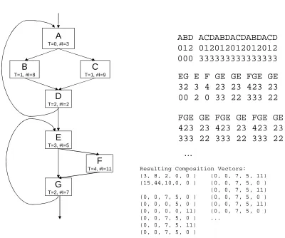
A
T=0, #I=3
B
T=1, #I=8
C
T=1, #I=9
D
T=2, #I=2
E
T=3, #I=5
G
T=2, #I=7
F
T=4, #I=11
ABD ACDABDACDABDACD
012 012012012012012
000 333333333333333
EG E F GE GE FGE GE
32 3 4 23 23 423 23
00 2 0 33 22 333 22
FGE GE FGE GE FGE GE
423 23 423 23 423 23
333 22 333 22 333 22
…
Resulting Composition Vectors: (3, 8, 2, 0, 0 ) (0, 0, 7, 5, 11) (15,44,10,0, 0 ) (0, 0, 7, 5, 0 ) (0, 0, 7, 5, 11) (0, 0, 7, 5, 0 ) (0, 0, 7, 5, 0 ) (0, 0, 0, 5, 0 ) (0, 0, 7, 5, 11) (0, 0, 0, 0, 11) (0, 0, 7, 5, 0 ) (0, 0, 7, 5, 0 ) ...
(0, 0, 7, 5, 11) (0, 0, 7, 5, 0 )
We use an LRU stack to track the segments.
Suppose the window size is 3
(0, 0, 7, 5, 0 )
(0, 0, 7, 5, 0 ) (0, 0, 0, 5, 0 )
(0, 0, 7, 5, 0 ) (0, 0, 0, 5, 0 ) (0, 0, 0, 0, 11)
(0, 0, 0, 5, 0 ) (0, 0, 0, 0, 11) (0, 0, 7, 5, 0 ) (0, 0, 0, 5, 0 ) (0, 0, 0, 0, 11) (0, 0, 7, 5, 0 ) (0, 0, 7, 5, 11)
(0, 0, 7, 5, 0 )
(0, 0, 0, 0, 11) (0, 0, 7, 5, 11)
(0, 0, 0, 0, 11) (0, 0, 0, 0, 11) (0, 0, 7, 5, 11) (0, 0, 7, 5, 11) (0, 0, 7, 5, 0 )
(0, 0, 7, 5, 0 ) (0, 0, 7, 5, 11)
(0, 0, 7, 5, 0 ) (0, 0, 7, 5, 11) (0, 0, 7, 5, 0 ) (0, 0, 7, 5, 11)
(0, 0, 0, 0, 11) (0, 0, 7, 5, 11) (0, 0, 7, 5, 0 )
(0, 0, 0, 0, 11) (0, 0, 0, 0, 11)
(0, 0, 7, 5, 0 )
(0, 0, 0, 0, 11) (0, 0, 7, 5, 11) (0, 0, 7, 5, 0 ) (0, 0, 7, 5, 0 ) (0, 0, 7, 5, 11)
(0, 0, 0, 0, 11) (0, 0, 7, 5, 0 )
(0, 0, 7, 5, 0 ) (0, 0, 7, 5, 0 )
(3, 8, 2, 0, 0 ) (15,44,10,0,0 )
(15,44,10,0,0 )
(3, 8, 2, 0, 0 )
(0, 0, 0, 0, 11) (0, 0, 7, 5, 11)
(0, 0, 0, 0, 11) (0, 0, 0, 0, 11) (0, 0, 7, 5, 11) (0, 0, 7, 5, 0 )
(0, 0, 7, 5, 11) (0, 0, 7, 5, 0 ) (0, 0, 7, 5, 11)
(0, 0, 0, 0, 11) (0, 0, 7, 5, 11) (0, 0, 7, 5, 0 )
(0, 0, 0, 0, 11) (0, 0, 7, 5, 0 )
(0, 0, 0, 0, 11) (0, 0, 7, 5, 11) (0, 0, 7, 5, 0 ) (0, 0, 7, 5, 0 ) (0, 0, 7, 5, 11)
(0, 0, 0, 0, 11) (0, 0, 7, 5, 0 )
(0, 0, 7, 5, 0 )
Resulting Intervals:
ABD ACDABDACDABDACD EG E FGE
GEFGEGEFGEGEFGEGEFGEGE
Since the patterns we are looking for are inherently similar to those of basic blocks but at a larger granularity, we create a new LRU stack and update it with segment composition vectors to facilitate combining segments. We enforce a maximum size for the LRU stack and the oldest entry will be discarded when the stack size exceeds this limit. Hence, vectors that recur with a stack hit depth larger than the maximum stack depth (referred to as window size) will be treated as if this is the first time they are observed. If a composition vector hits in the stack, this implies it is one of the small group of segments that is currently being executed. If a composition vector misses in the LRU stack, this is an indication of a possible phase boundary and we mark it as the beginning of a new interval. An interval is a set of several consecutive segments. When formed this way, the resulting intervals are unlikely to cross any natural phase boundaries. Figure 4.4 shows how the LRU stack is updated and segments are merged. The first stack shows the state when the first two segments have been pushed onto the stack and the third one is being accessed.
studied in order to generate intervals longer than 1 million instructions. When combined, these intervals account for over 99% of the entire program execution. gcc is the only ex-ception, where we needed 60 iterations and the resulting intervals longer than 0.1 million instructions only accounts for 96.4% of its execution. Our experiments show that ignoring such a small part of the program does not introduce any appreciable error.
Note that while we were seeking exact basic block type ID matches in the first level of our pattern searching algorithm, this requirement needs to be relaxed when we are searching for composition vector matches. To allow for some tolerance in our LRU stack based algorithm, we normalize the composition vectors with the sum of all dimensions before comparing them. In this way, if two different segments is just the same section of code that have different trip counts, they can be considered as part of the same segment. When comparing two normalized compositions, they are considered to be “similar” if their Manhattan distance [48] is less than 5% of the maximum possible value. The Manhattan distance between two composition vectors is the sum of the differences of their corresponding components. In Figure 4.5, the upper portion shows how composition vectors before and after normalization and the lower portion shows we calcuate their Manhattan distance. Notice that the first and second segments, which wouldn’t have been merged using exact match, will be merged into a single interval since their Manhattan distance is 0.04 (within 2%).
4.4.3.4 Hierarchical Clustering
1. ABD
2. ACDABDACDABDACD 3. EG
4. E 5. F 6. GE 7. FGE
: (3, 8, 2, 0, 0 ) -> (0.23,0.62,0.15,0, 0 ) : (15,44,10,0, 0 ) -> (0.22,0.64,0.14,0, 0 ) : (0, 0, 7, 5, 0 ) -> (0, 0, 0.58,0.42,0 ) : (0, 0, 0, 5, 0 ) -> (0, 0, 0, 1, 0 ) : (0, 0, 0, 0, 11) -> (0, 0, 0, 0, 1 ) : (0, 0, 7, 5, 0 ) -> (0, 0, 0.58,0.42,0 ) : (0, 0, 56,50,44) -> (0, 0, 0.37,0.33,0.29) For example, we list some of the Manhattan distances between two
segments/intervals:
1. And 2.: diff vec: (0.01,0.02,0.01,0, 0 ), Manhattan Dist=0.04; 1. And 3.: diff vec: (0.23,0.62,0.43,0.42,0 ), Manhattan Dist=1.80; 1. And 4.: diff vec: (0.23,0.62,0.15,1 ,0 ), Manhattan Dist=2;
Figure 4.5: Calculating Manhattan Distance between segments/intervals.
of the execution. In the final step of our phase analysis framework, we perform clustering on the intervals we generated from LRU stack hit patterns to form phases.