Abstract
PATI, SWAMY. Effects of Subsurface Flows on Wetland Restoration at Juniper Bay and Surrounding Area. (Under the direction of Rodney L. Huffman.)
The North Carolina Department of Transportation purchased a 270-hectare,
roughly elliptical tract of agricultural land, known as Juniper Bay (a Carolina Bay), to
convert to wetlands as part of their wetlands mitigation program. Preliminary water
balance work suggested that there are significant flows of groundwater entering and
leaving the tract. This study was initiated to examine the subsurface potentials and
determine the degree to which a ditch around the perimeter of the tract controls the lateral
fluxes of groundwater in the surficial aquifer. Five nests of piezometers were installed
along each of four 150-m transects crossing the perimeter ditch at approximately the
major and minor axes of the tract, which correspond to the suspected maxima of influx
and efflux. Deep soil cores (up to 13 m) were collected along each transect to guide
placement of piezometers for monitoring hydraulic heads. Piezometer water levels were
recorded at 15-minute intervals. Meteorological data were collected with an on-site
weather station.
Models were developed for the four transects using Visual MODFLOW. Models
were calibrated with observed groundwater pressure heads. Maximum absolute error in
the calibration process was 0.5 m. The modeling results suggested that the ditch drained
water from the surficial system from both sides. In the deeper sand layers, there was an
indication of groundwater flowing into the bay at NW and NE transects. Groundwater
flows in the SW transect indicated outflows. The SE transects showed water draining into
conditions after the interior ditch system was blocked. Simulation results showed
groundwater inflows through the NW, NE, and SE transect, and groundwater outflows
through SW transect. The lateral influence of the perimeter ditch had a maximum of
approximately of 100 m, observed at the SW transect, and a minimum of 30 m, observed
at the SE transect. The extent of influence of the perimeter ditch was also dependent on
the weather conditions, showing more influence in summer months compared to winter
months. Influence of the perimeter ditch was entirely in the upper sands at the NE and SE
transects, but some influence was seen in the middle sand layers at the NW and SW
transects. Groundwater flow estimates from the transects were extrapolated over the
whole perimeter of Juniper Bay to obtain net groundwater inflow. Net groundwater
inflow was approximately 125 mm for the time period of 1 January 2004 to 30 June
2004.
To develop recommendations for maintaining the perimeter ditch, the models
were run for various scenarios focused on water levels in the perimeter ditch. Control
levels were imposed on the ditch and options were investigated. A water level of 35.9 m
MSL was identified as a critical point of control of the perimeter ditch. Controlling the
water level in the perimeter ditch at 35.9 m will minimize offsite impacts and result in
Effects of Subsurface Flows on Wetland
Restoration at Juniper Bay and Surrounding Area
by
SWAMY PATI
A dissertation submitted to the Graduate Faculty of North Carolina State University
in partial fulfillment of the requirements for the Degree of
Doctor of Philosophy
BIOLOGICAL AND AGRICULTURAL ENGINEERING
Raleigh
2006
APPROVED BY:
__________________________ _________________________ Rodney L. Huffman R. Wayne Skaggs Chair of Advisory Committee Member of Advisory Committee
__________________________ _________________________ Michael J. Vepraskas Michael R. Burchell II Member of Advisory Committee Member of Advisory Committee
__________________________
Dedication
Biography
Swamy Pati was born in 1977 in Pitapuram, Andhra Pradesh in India. His father
works with Indian Railways as Junior Engineer – Electrical, and mother is a house wife.
His only brother was graduated with Masters of Computer Applications and working a
software engineer in New Jersey, USA. Parents live in Kakinada, India.
He was bought up in Vijayawada, Andhra Pradesh in India where he did
schooling in Railway Mixed High School and Nalanda Junior College. He graduated
from High school in 1994. He graduated with a Bachelor of Technology in Agricultural
Engineering in August 1999 from Acharya NG Ranga Agricultural University.
He started MS at Utah State University in Jan 2001 in Biological and Irrigation
Engineering and graduated in August 2002. He worked with Dr. Wynn Walker in the
project called IRRINET developing web-based course on Principles of Irrigation
Engineer. After completing MS, with the quest for knowledge and interest he joined for
PhD program in Biological and Agricultural Engineering at North Carolina State
University. His concentration was in Environmental Engineering, he worked with Dr.
Rodney L. Huffman in a project dealing with groundwater aspects at a wetland
restoration site.
During his stay at NC State, he was awarded International Student Scholarship for
2004 by Rotary Club. He was initiated in Honor Society of Agriculture – Gamma Sigma
Delta in 2006. He is a student member of professional societies American Society of
Agricultural and Biological Engineers (ASABE) and National Groundwater Association
Apart from academics, he was active in social activities and served as
Vice-President of MAITRI – Indian Graduate Student Association at NC State University for
year 2004. He is also a member of charity organization – Two Cents of Hope, helps for
educational needs of under privileged children in India. He likes playing cricket and
volley ball. His other hobbies include spending time with friends, movies, music, and
dance. He likes traveling and visited many parts of US in just 4 years. His mother tongue
Acknowledgements
I sincerely thank my adviser Dr. Rod Huffman, for giving me the opportunity to
work with him for my PhD program. Thanks to him for his immense support, patience,
understanding, and help throughout my Doctoral program.
There are so many people to whom I have to express my gratitude for successful
completion of my PhD. I would like to thank my committee members, Dr. Wayne
Skaggs, Dr. Mike Vepraskas, Dr. John Parsons, Dr. Mike Burchell, and Dr. Gary
Roberson. Thanks to Dr. Skaggs for his support and help to pass through my difficult
times when I had to repeat my Preliminary Exams. Sincere thanks to Dr. Vepraskas for
his constant encouragement. Special thanks to Dr. Parsons, who provided me with useful
suggestions during my initial stages of groundwater modeling efforts. Dr. Burchell,
thanks for joining the graduate committee, though it was tail end of my program. Thanks
to Dr. Gary Roberson for being Minor Representative of the graduate committee.
I would like to thank research technician, Alex Adams, for his help in field work
and lab experiments. I would like to thank Pete, Alex, and Andrew, who helped me in
different stages of my field and lab work. I also would like to thank colleagues in Juniper
Bay Research group. Thanks to Mark Wilsnack for his timely suggestions in modeling
part of my research.
I thank Dr. Dan Willits (DGP of BAE), Kathy Logan and Heather Gordon
(graduate secretaries of BAE) during my stay at NC State, for their help in administrative
front. Also I would like to thank Graduate Student community in the Dept of BAE.
Thanks to all my roomies and friends during my stay at NC State, especially
Srinivas, Amit Acharya, Kannan AJ, and Vikrant Mathur for their help and support
Table of Contents
List of Tables ... ix
List of Figures ... xi
Chapters 1. Introduction ...1
2. Literature Review ...6
2.1. Carolina Bays ...6
2.2. Juniper Bay ...9
2.3. Groundwater Modeling...10
3. Characterizing Subsurface flows ...13
3.1. Establishing Transects ...13
3.2. Soil Coring ...14
3.3. Soil Profiling...16
3.4. Saturated Hydraulic Conductivity Tests ...20
3.5. Installation of Piezometers...22
3.6. Water Level Monitoring System...24
3.7. In-situ Hydraulic Conductivity Tests...27
3.8. Data Collection ...30
3.9. Summary ...35
4. Modeling and Analysis of Subsurface flows at the four transects...37
4.1. Model Development...37
4.2. Analysis of Modeling Results...45
4.3. Extended Model ...51
4.4. Summary ...72
5. Recommendations for Perimeter Ditch Management...75
5.1. Control Levels on the Perimeter Ditch ...75
5.3. Analysis of Control Levels at the NE Transect ...83
5.4. Analysis of Control Levels at the SE Transect ...89
5.5. Analysis of Control Levels at the SW Transect...95
5.6. Net Groundwater Flow in Juniper Bay ...101
5.7. Summary ...102
6. Conclusion and Recommendations for Future Research ...104
References...108
List of Tables
Chapter 3
Table 3.1 Example of Ksat table describing soil color, texture and saturated
hydraulic conductivity at NW-EX-75 core location ...22
Table 3.2 Screened depths of piezometers...24
Table 3.3 Ksat values from slug tests...29
Table 3.4.1 NW transect water level data on 4 April 2004...32
Table 3.4.2 NE transect water level data on 4 April 2004...33
Table 3.4.3 SE transect water level data on 4 April 2004...34
Table 3.4.4 SW transect water level data on 4 April 2004 ...35
Chapter 4 Table 4.1 Elevations for five layers for the four transect models ...40
Table 4.2 Effective Saturated Hydraulic Conductivity (m/sec) of different layers ...43
Table 4.3 Summary of Groundwater flows...71
Table 4.4 Influence of the perimeter ditch...74
Chapter 5 Table 5.1 Net flow at the NW transect for different control levels ...81
Table 5.2 Net flow at the NE transect for different control levels...87
Table 5.3 Net flow at the SE transect for different control levels ...93
Table 5.4 Net flow at the SW transect for different control levels ...99
Table 5.5 Net groundwater flows for 01 January 2004 to 30 June of 2004...101
Table 5.6 Summary of Critical Ditch Control Levels...102
Appendix A Table A.1 Ksat table for the Northwest (NW) transect ...110
Table A.2 Ksat table for the Northeast (NE) transect ...114
Table A.3 Ksat table for the Southeast (SE) transect ...119
Table A.4 Ksat table for the Southwest (SW) transect...122
Appendix B Table B.1 Example for estimating effective conductivity for NW-EX-75 in layer 1...131
Appendix C
List of Figures
Chapter 1
Figure 1.1 Aerial image of Juniper Bay from 1993 (USDA-FSA) ...3
Figure 1.2 Conceptualization of stratigraphy at Juniper Bay ...4
Chapter 2 Figure 2.1.1 Arial Photo of Carolina Bays covering around five hundred middle near Myrtle Beach in Horry County, South Carolina ...7
Chapter 3 Figure 3.1.1 Elevation Map of Juniper Bay...14
Figure 3.2.1 Schematic locations of each transect...15
Figure 3.2.2 Core locations on each transect ...16
Figure 3.3.1 Soil Profiles at the NW transect ...17
Figure 3.3.2 Soil Profiles at the NE transect...18
Figure 3.3.3 Soil Profiles at the SE transect ...18
Figure 3.3.4 Soil Profiles at the SW transect ...19
Figure 3.3.5 Legend ...19
Figure 3.4.1 Schematic for Ksat apparatus ...21
Figure 3.6.1 Water level monitoring system...24
Figure 3.6.2 Schematic diagram of a monitoring unit assembly ...26
Figure 3.6.3 Monitoring unit in its enclosure ...27
Figure 3.8.1 Hydraulic heads from the NW transect, 4 April 2004...31
Figure 3.8.2 Hydraulic heads from the NE transect, 4 April 2004 ...32
Figure 3.8.3 Hydraulic heads from the SE transect, 4 April 2004...33
Figure 3.8.4 Hydraulic heads from the SW transect, 4 April 2004 ...34
Figure 3.8.5 Legend ...35
Chapter 4 Figure 4.1.1 Model setup for the NW transect...41
Figure 4.1.2 Correlation Coefficient between the observed and calculated heads ...43
Figure 4.1.3 Comparison plot between observed and calculated ...44
Figure 4.2.2 Equipotential Lines for 13 May 2004 at the NW transect...46
Figure 4.2.3 Equipotential Lines for 15 February 2004 at the NE transect ...48
Figure 4.2.4 Equipotential Lines for 13 May 2004 at the NE transect ...48
Figure 4.2.5 Equipotential Lines for 15 February 2004 at the SE transect...49
Figure 4.2.6 Equipotential Lines for 13 May 2004 at the SE transect...49
Figure 4.2.7 Equipotential Lines for 15 February 2004 at the SW transect ...50
Figure 4.2.8 Equipotential Lines for 13 May 2004 at the SW transect ...50
Figure 4.3.1 Extended Model shown for the NW transect ...52
Figure 4.3.2 Calibration plot example at the NW transect ...54
Figure 4.3.3 Equipotential Lines on 15 February 2004 at the NW Transect extended model ...55
Figure 4.3.4 Heads in the three conducting layers at the NW transect on 15 February 2004 ...55
Figure 4.3.5 Equipotential Lines on 13 May 2004 at the NW Transect extended model ...56
Figure 4.3.6 Heads in the three conducing layers at the NW on 13 May 2004 ...56
Figure 4.3.7 Inflow rates at the NW transect ...57
Figure 4.3.8 Calibration plot example at the NE transect...58
Figure 4.3.9 Equipotential Lines on 15 February 2004 at the NE Transect extended model ...59
Figure 4.3.10 Heads in the three conducting layers at the NE transect on 15 February 2004 ...60
Figure 4.3.11 Equipotential Lines on 13 May 2004 at the NE Transect extended model ...60
Figure 4.3.12 Heads in the three conducing layers at the NE on 13 May 2004 ...61
Figure 4.3.16 Heads in the three conducting layers at the SE transect on
15 February 2004 ...64
Figure 4.3.17 Equipotential Lines on 13 May 2004 at the SE Transect extended model ...65
Figure 4.3.18 Heads in the three conducing layers at the SE on 13 May 2004 ...65
Figure 4.3.19 Inflow rates at the SE transect ...66
Figure 4.3.20 Calibration plot example at the SW transect ...67
Figure 4.3.21 Equipotential Lines on 15 February 2004 at the SW Transect extended model ...67
Figure 4.3.22 Heads in the three conducting layers at the SW transect on 15 February 2004 ...68
Figure 4.3.23 Equipotential Lines on 13 May 2004 at the SW Transect extended model ...68
Figure 4.3.24 Heads in the three conducing layers at the SW on 13 May 2004 ...69
Figure 4.3.25 Outflow rates at the SW transect ...70
Figure 4.3.26 Comparison of Monthly Flows at the four transects ...71
Figure 4.4.1 Summary of flow direction in significant sand layers...74
Chapter 5 Figure 5.2.1 Spatial distribution of heads in surficial sand layer at the NW transect for different ditch control levels on 15 February 2004...77
Figure 5.2.2 Spatial distribution of heads in surficial sand layer at the NW transect for different ditch control levels on 13 May 2004...77
Figure 5.2.3 Spatial distribution of heads in middle sand layer at the NW transect for different ditch control levels on 15 February 2004...78
Figure 5.2.4 Spatial distribution of heads in middle sand layer at the NW transect for different ditch control levels on 13 May 2004...79
transect for different ditch control levels on 13 May 2004...80 Figure 5.2.7 Net inflows at the NW transect from different control levels ...81 Figure 5.3.1 Spatial distribution of heads in surficial sand layer at the NE
transect for different ditch control levels on 15 February 2004...83 Figure 5.3.2 Spatial distribution of heads in surficial sand layer at the NE
transect for different ditch control levels on 13 May 2004...84 Figure 5.3.3 Spatial distribution of heads in middle sand layer at the NE
transect for different ditch control levels on 15 February 2004...85 Figure 5.3.4 Spatial distribution of heads in middle sand layer at the NE
transect for different ditch control levels on 13 May 2004...85 Figure 5.3.5 Spatial distribution of heads in deep sand layer at the NE
transect for different ditch control levels on 15 February 2004...86 Figure 5.3.6 Spatial distribution of heads in deep sand layer at the NE
transect for different ditch control levels on 13 May 2004...86 Figure 5.3.7 Net inflows at the NW transect from different control levels ...87 Figure 5.4.1 Spatial distribution of heads in surficial sand layer at the SE
transect for different ditch control levels on 15 February 2004...89 Figure 5.4.2 Spatial distribution of heads in surficial sand layer at the SE
transect for different ditch control levels on 13 May 2004...90 Figure 5.4.3 Spatial distribution of heads in middle sand layer at the SE
transect for different ditch control levels on 15 February 2004...91 Figure 5.4.4 Spatial distribution of heads in middle sand layer at the SE
transect for different ditch control levels on 13 May 2004...91 Figure 5.4.5 Spatial distribution of heads in deep sand layer at the SE
transect for different ditch control levels on 15 February 2004...92 Figure 5.4.6 Spatial distribution of heads in deep sand layer at the SE
transect for different ditch control levels on 13 May 2004...96 Figure 5.5.3 Spatial distribution of heads in middle sand layer at the SW
transect for different ditch control levels on 15 February 2004...97 Figure 5.5.4 Spatial distribution of heads in middle sand layer at the SW
transect for different ditch control levels on 13 May 2004...97 Figure 5.5.5 Spatial distribution of heads in deep sand layer at the SW
transect for different ditch control levels on 15 February 2004...98 Figure 5.5.6 Spatial distribution of heads in deep sand layer at the SW
transect for different ditch control levels on 13 May 2004...98 Figure 5.5.7 Net inflows at the NW transect from different control levels ...99 Figure 5.6.1 Net groundwater flows for 01 January 2004 to 30 June of 2004 ...102
Appendix B
Chapter 1
Introduction
The North Carolina Department of Transportation purchased a 270-hectare parcel
of agricultural land, Juniper Bay (a drained Carolina Bay), to convert into wetland as part
of their wetland mitigation program. The success rate for wetland conversion has been
relatively low due to shortcomings in site assessment, identification of potential
functions, methodologies to restore wetland functions, and effective assessment of
progress of functional restoration, which are the factors that are set by the US Army
Corps of Engineers. The Department of Soil Science at North Carolina State University,
in collaboration with several other departments (Biological and Agricultural Engineering,
Forestry, and Botany), started a research project to address those shortcomings in the
study of restoration success in Juniper Bay. This research will help to define the
characteristics of a site that affect the success of a project. The preliminary water balance
work (Kreiser et al., 2003) on this project suggested that there is a significant amount of
groundwater entering and leaving the bay. Water budget work showed a wide variation in
estimates of groundwater inflows, which was mainly attributed to uncertainty in the
estimation of evapotranspiration. When groundwater potentials were examined around
the site and data suggested the possibility of significant lateral subsurface fluxes, it was
decided to look into the groundwater situation in more detail. Due to the sparseness of the
research project was initiated to examine the subsurface potentials and determine the
degree to which a ditch around the perimeter of the tract controls the lateral fluxes of
groundwater in the surficial aquifer.
Objectives:
1. Characterize the subsurface flows at the perimeter of the Bay.
2. Determine the degree and modes of interaction of the perimeter ditch of
the Bay with the partially confined sand strata.
3. Model the subsurface flows in the Bay area and assess the impacts of these
flows on the surrounding area.
4. Develop management recommendations for the perimeter ditch
Background
Carolina Bays are oval-shaped wet depressions with a northwest-southeast
orientation (Howard, 1977). They are spread throughout the eastern coastal plain of the
United States from Delaware to Florida. Some are filled with water and named as lakes.
Many of them are in a vegetative wetland state. According to the theories of different
hydrologists, the hydrology of Carolina Bays is influenced by the inputs from the
subsurface flows and by the underlying fine-textured sediments that restrict vertical
movement of water. Knight et al. (1989), Newman and Schalles (1990), Lide et al.
(1995), and O’ney et al. (1999) have studied the complex hydrology of Carolina Bays and
have shown the complex subsurface interactions with the surrounding area. Their studies
also indicated there was local depressional hydrology superimposed on the regional
Juniper Bay is located in Robeson County, North Carolina. Figure 1 shows the
location and elliptical shape of Juniper Bay, a common characteristic of Carolina Bays.
Initially a wetland, Juniper Bay was drained for industrial purposes in the early 1960s and
it was intensively drained for agriculture in the late 1970s. As of 2000, it had about 270
ha of drained and intensively managed agricultural land that was not jurisdictional
wetland due to its status as prior converted agricultural land. Prior to ditching, surface
runoff apparently left the bay through an area in the southern portion where the rim is
very low or missing. The ditch system now conveys both surface and subsurface drainage
to the outlet shown in Figure 1.1.
Main canals
Laterals Outlet
Perimeter Ditch
A conceptual profile at Juniper Bay is shown in figure 2. This illustrates the
expected types of formations at Juniper Bay. The stratigraphic work done to date
identified the Black Creek Confining Unit (BCCU) at a depth of 6–10 m throughout the
bay area. The BCCU is the fine-textured material underlying Juniper Bay. It restricts the
water movement and can be considered an effective bottom of the system of interest. The
overlying strata consist of discontinuous clay layers with unconfined and partially
confined sands. Core work done to date suggests that there are typically one or two
confined sand layers above the Black Creek Confining Unit. The property boundary was
approximated by the perimeter ditch. The study area extends some distance outside the
ditch, which was needed to assess interactions across the property/ditch boundary.
Figure 1.2: Conceptualization of stratigraphy at Juniper Bay
The perimeter ditch encircles the entire bay. It may have a significant influence on
the hydrology of the bay. It could influence the flows in the surficial aquifer and intercept
shallow flows between the interior and exterior of the bay. It can effectively drain
sands may or may not be affected by the perimeter ditch. Determining its depth of
influence is one of the main objectives of the project. This study will investigate whether
the ditch could be eliminated, which could increase the converted wetland area by about
20 hectares.
To estimate the lateral ground water flows entering and leaving the bay, a
groundwater potential monitoring system with good resolution was needed. Knowledge
of the hydraulic heads across the perimeter section, along with hydraulic conductivities of
the strata, would permit assessment of the impacts of the bay’s drainage system on the
surrounding area. Knowledge of the function of the perimeter ditch would provide a basis
for recommendations on ditch management.
Groundwater modeling will be used in analyzing the subsurface flows for the
collected data, and also applying extreme conditions for suggesting recommendations for
future perimeter ditch management. The following chapters will discuss how these
objectives are achieved, including data collection, modeling efforts and presentation of
Chapter 2
Literature Review
2.1 Carolina Bays
Juniper Bay is one of the typical isolated wetlands called Carolina Bays. Carolina
Bays are oval shaped wet depressions with a northwest-southeast orientation (Howard,
1997). They are spread throughout the eastern Coastal Plain of the United States from
Delaware to Florida. Figure 2.1.1 shows an Aerial photo, from 1903, of cluster of
Carolina Bays near Myrtle Beach, South Carolina. Some are filled with water and named
as lakes. These Bays are estimated to be at least 40,000 years old at deeper soils (2.3m)
and atleast 5,750 years at shallow depths (1.05m). They have northwest to southeast
orientation and they vary in size from few hundred feet to three of four miles in longest
diameter. Many are bordered by rim of sands. Many of them are in a vegetative wetland
state. There are several theories explaining their origin. Most important of them are
which explain the origin from meteorites and wind action.
Origination of Carolina Bays
Johnson (1936) suggested that shape and orientation, as well as presence of sandy
rims can be attributed to wind and wave action and depressions are attributed to the
artesian process. Prouty (1952) attributed the origin of the Bays to the influence of comet
or asteroidal body entering the earth atmosphere at an oblique angle from a relatively
northwesterly direction. Thom (1970) explained the origin with the Humate that allows
depressions, orientated later by wind and wave action. Eyton & Parkhurst (1975)
considered the theory stated by Prouty (1952) and then they stated finally that comets are
the cause for the creation of Carolina Bays. Kaczorowski (1977) ruled out the
extraterrestrial theory as a cause for Bay formation and supported Thom water table
perching theory. He suggested that the only requirement for Bay existence is poor
drainage leading to ponding mechanisms.
Figure 2.1.1: Arial Photo of Carolina Bays covering around five hundred middle near Myrtle
Beach in Horry County, South Carolina.
Hydrology of Carolina bays
very poorly drained in the lowest elevation portions. Most of the bays are jurisdictional
wetlands. Some bays have surface runoff outlets, but the majority likely does not, some
have dispersed overland flows as outlets and the others have stream channels.
According to the theories of different hydrologists, the hydrology of Carolina
Bays is influenced by the inputs from the subsurface flows and by the underlying
fine-textured sediments, which restrict the vertical movement of water. Sharitz and Gibbons
(1982) showed that the hydroperiods were dominated by rainfall inputs and evaporation
outputs. Knight et al. (1989), Newman and Schalles (1990), Lide et al. (1995), and O’ney
et al. (1999) have studied the complex hydrology of Carolina Bays and have shown the
complex subsurface interactions with the surrounding area. Their studies also indicated
there was local depressional hydrology superimposed on the regional subsurface
hydraulic gradients of the landscape in which the bay occurred. There was local
depressional hydrology superimposed on the regional subsurface hydraulic gradients of
the landscape in which the bay occurred. Lide etal. (1995) and O’ney et al. (1999) found
that the topography of the subsurface was similar to the surface topography. Hydraulic
gradient into the bay resulted in subsurface flows along sandy layers overlying
fine-textured layers. Gradients are into the bay in the wet season. Lide et al. (1995) concluded
that there is significant groundwater recharge in the dry periods of late spring/early
summer at Thunder Bay, SC. Chapel bay was studied by O’ney et al. (1991), which
provided some recharge, but drying was dominated by ET losses. Schalles et al. (1989)
suggested that chemistry of water and soils in clay-based Carolina bays indicate a
rainwater-dominated system characteristic of perched water settings. Landscape position,
individual bay hydrology and response to rainwater. Bays are likely both recharge and
discharge depending on bay water levels in relation to the regional water table (Schalles,
1979).
2.2 Juniper Bay
Juniper Bay is located in Robeson County, North Carolina. As a typical
characteristic of Carolina bay, Juniper bay is elliptical in shape. Initially a wetland,
Juniper Bay was drained for industrial purposes in the early 1960s and it was intensively
drained for agricultural purposes in the late 1970s. As of 2000, it had about 270 ha of
drained and intensively managed agricultural land that is not jurisdictional wetland due to
its status as prior converted agricultural land.
Zanner (2003) concluded that Juniper Bay is formed in 5-8 m of Pliocene aged
Duplin-Yorktown Formation sediments that are underlain by Cretaceous aged Donoho
Creek and Bladen Formation of the Black Creek Group. Subsurface sediment topography
is observed to be irregular with the newer sediment filling in erosional channels as it was
deposited. Luginbuhl (2003) studied the groundwater hydrology at Juniper bay prior to
restoration and her study suggested that groundwater flows may be entering from the
northwest and southeast boundaries and leaving from the northeast and southwest
boundaries. Kreiser (2003) studied water budget at Juniper bay and reported that there are
significant amount of groundwater flows coming into the site. He estimated groundwater
flows were in the range of 171 mm to 563 mm, though the estimates are very uncertain
there were significant groundwater flows entering into the site. If the subsidence is taken
into account with these groundwater inflows there is a possibility of formation of lake
instead of a wetland.
2.3 Modeling
Groundwater models were approached typically for two main reasons (Fetter,
2001), 1) to understand why a flow system is behaving in a particular observed manner,
and 2) to predict how a flow system will behave in the future. Initially analytical models
were used for groundwater modeling and then numerical models were introduced.
MODFLOW (McDonald and Harbaraugh, 1984) is one of the numerical models that use
finite difference technique to solve the governing flow equation.
It was developed by USGS in 1998 and then updated with a new version in 2000.
It was integrated with surface unsaturated flow models and developed
MODFLOW-SURFACT by HydrGeoLogic Inc., in 2002. MODFLOW is widely used software for
groundwater fate and transport modeling. It can be used for both two dimensional and
three dimensional groundwater flow modeling.
McDonald and Harbaraugh (2000) explained concepts of groundwater flow
concepts in MODFLOW. The partial-differential equation of groundwater flow used in
MODFLOW is given in Equation 2.3.1. MODFLOW uses finite-difference method to
Kxx h Kyy h Kzz h W Ss h
x x y y z z t
⎛ ⎞
∂ ⎛ ∂ ⎞+ ∂ ∂ + ∂ ⎛ ∂ ⎞+ = ∂
⎜ ⎟
⎜ ⎟ ⎜ ⎟
∂ ⎝ ∂ ⎠ ∂ ⎝ ∂ ⎠ ∂ ⎝ ∂ ⎠ ∂ (2.3.1)
Kxx, Kyy, and Kzz - Values of hydraulic conductivities along the x, y, and z coordinate axes (L/T)
h - Potentiometric head (L)
W - Volumetric flux per unit volume representing sources and/or sinks of water, with W<0.0 for flow out of the groundwater system, and W>0.0 for flow in (T-1)
Ss - Specific storage of the porous media material (L-1) t - Time (T)
Sonenshein (2001) studied methods to quantify seepage beneath Levee 30,
Miami-Dade County, Florida. His study used a 2-D finite difference groundwater model
and simple application of Darcy’s Law to quantify these flows. Accuracy in estimating
groundwater flows was less due to uncertainty in the horizontal conductivity in the main
flow zone of the Biscayne aquifer. Simulated lateral groundwater flows were highest in
the wet seasons.
Moreno et. al., (2003) compared the decision tree approach and automated
parameter estimation approach to calibrate groundwater flow model. Their study
concluded that the combination approach of trial and error calibration and automated
parameter estimation would be ideal approach for calibration groundwater flow models.
Andre (2005) researched on using geochemical data and modeling to enhance
understanding the groundwater flow in a regional deep aquifer, aquifer basin, south-west
of France. They concluded that geochemical data can be used to identify deep
groundwater flow patterns when geology and hydrogeology data is scarce to provide
Karahan (2005) proposed a transient groundwater modeling using spreadsheet.
His study suggested that spreadsheet modeling for simple groundwater scenarios is in
Chapter 3
Characterizing Subsurface flows
This chapter discusses methodology to accomplish the first objective,
characterizing subsurface flows at the perimeter of Juniper Bay. It details the procedure
followed in establishing transects, collecting cores and analyzing them for determining
depths for the installation of piezometers. This chapter also explains development and
deployment of water level monitoring systems at each piezometer nest. Furthermore, it
presents preliminary analyses of water level data collected at each transect, focused on
lateral and vertical fluxes along with influence of perimeter ditch.
3.1 Establishing Transects
From the topographic information shown in Figure 3.1.1, one can observe that the
elevations to the northwest (NW) and southeast (SE) are higher than the elevations to the
southwest (SW) and northeast (NE). A study of groundwater flows by Luginbuhl (2003)
also suggests higher elevations on the SW and NE. The variation in the surface elevations
at the interior of the bay is small, approximately 0.6 m over 2400 m, in comparison to the
exterior of the bay which is approximately 1 m from NE transect to SE transect. At NW
and SE transects the differences in surface elevation from interior 75 m to exterior 75 m
of the bay are approximately 1m, exterior being on the higher elevation. Going further
out to the NW and SE, the land surface rises even more, which suggests that subsurface
four transects are designated as Northwest (NW), Southwest (SW), Southeast (SE), and
Northeast (NE), as shown in Figure 3.2.1.
Transect Locations
Figure 3.1.1: Elevation map of Juniper Bay (8x vertical exaggeration). Arrows indicate the
proposed direction of subsurface flux.
3.2 Soil Coring
At each transect, sediment cores were collected at five different points on each
transect as shown in Figure 4b. Three sediment cores were collected at the interior of the
bay at 5, 25, and 75 m from the center of the ditch. Similarly, two sediment cores were
collected at the exterior of the bay at 25 and 75 m from the center of the ditch. The drill
rig from the Department of Biological & Agricultural Engineering, North Carolina State
University, was used for the coring. Cores were collected using a 102-mm OD, 1.52-m
long core barrel inside 108-mm ID hollow stem auger. Plastic (cellulose acetate butyrate)
liners, 1.52 m x 87.8 mm OD x 0.79 mm wall thickness, facilitated handling and storage
of the cores. Cores were collected at each location to depths of approximately 8 to 11 m,
usually down to and penetrating the top of the Black Creek Confining Unit as shown in
the Figure 3.2.2. Coring through the Black Creek Confining Unit was very difficult at
most of the core locations.
Figure 3.2.1: Schematic locations of each transect. Purple dots represent the location of
piezometer nests. Brown squares represent location of preliminary cores collected for
25 m
75 m 5 m
Figure 3.2.2: Core Locations on each transect
3.3 Soil Profiling
Soil cores were characterized in the laboratory. Figures 3.3.1, 3.3.2, 3.3.3, and
3.3.4 show the stratigraphy at the NW, NE, SE, and SW transects, respectively. Figure
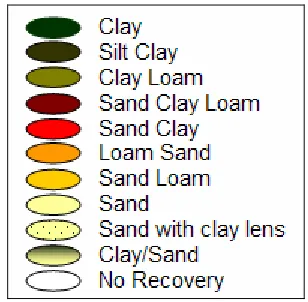
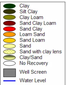
3.3.5 gives the legend for description of soil profiles. Colors represent the texture of the
sediments at each depth. Darker colors represent fine-textured sediments, like clayey
material, and light colors represent coarse-textured sediments, like sandy material. The
white sections indicate no recovery of sample. Those sections are assumed to be
non-cohesive sands. Significant difference in layers could be observed which helped in the
identifying sand layers that are the main water conducting layers. Horizontal distances in
the Figures (3.3.1, 3.3.2, 3.3.3, and 3.3.4) are not to scale, but vertical distances are to
scale. For the labels, EX represents exterior of the bay and IN represents interior of the
bay, while 05, 25, 50, and 75 are the corresponding distances (in meters) of the core
elevation at each of the core locations and perimeter ditch elevation and dimensions.
Ground surface elevations in meters, obtained from survey, are presented in the Figures
3.3.1 to 3.3.4.
Figure 3.3.2: Soil profiles at NE transect, legend is given in Figure 3.3.5
Figure 3.3.4: Soil Profiles at SW Transect, legend is given in Figure 3.3.5
Figure 3.3.5: Legend for Figures 3.3.1-4
The NW transect (Figure 3.3.1) had three distinguishable sand and coarse textured
layers. The top layer is considered to be surface layer to the depth of 2-4 m, and the
the deeper sands were found at the depths of 6-7 m and 8-10 m. The SW transect showed
the surface layer to the depth of 3-4 m. Deeper sand layers were found at the depths of
6-7 m and 8-9 m. The clay layers were discontinuous at all transects. This stratigraphy
agrees with the conceptual model of the subsurface.
3.4 Saturated Hydraulic Conductivity Tests
Samples from each significant stratum of the cores were inserted into 76 mm x
76 mm sleeves. Saturated hydraulic conductivity tests were conducted in the laboratory
using a constant-head apparatus. To prepare the cores to run for saturated hydraulic
conductivity (Ksat) tests, cores were saturated in water for 24 hours before setting up for
test. The saturated soil core was placed on a permeable base, wire mesh, inside a Buchner
funnel. Water from the constant head reservoir was allowed to flow through the sample
and the outflow from the bottom of the core was collected and measured using a
graduated cylinder, which has a measurement resolution of 1mL. Flow measurements
were taken at intervals of 4 hours. Measurements were taken until constant flow was
reached in two consecutive measurements. A schematic of the apparatus is shown in
Figure 3.4.1. This flow rate was used to estimate Ksat of each core sample. Ksat was
estimate using Darcy’s Law (Equation 3.4.1).
sat
QL K
At H
=
Δ (3.4.1)
Ksat – Saturated Hydraulic Conductivity
Q – Volume of the outflow during the time period t A – Cross-sectional area of core
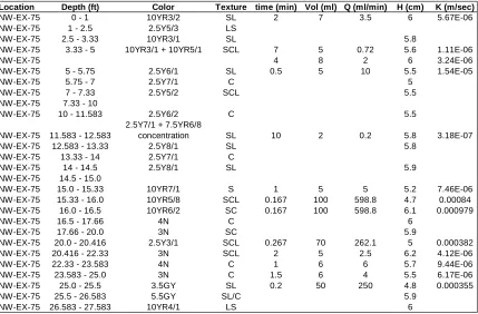
Table 3.4.1 gives the saturated conductivity values at different depths for the
NW-EX-75 core location. Appendix A gives all other tables corresponding to the different
core locations.
Figure 3.4.1: Schematic of Ksat Apparatus
Constant head
Graduated cylinder Soil Core
L = 76 mm H
Table 3.4.1: Example of Ksat table describing soil core color, texture and saturated sydraulic
conductivity at NW-EX-75 core location
Location Depth (ft) Color Texture time (min) Vol (ml) Q (ml/min) H (cm) K (m/sec)
NW-EX-75 0 - 1 10YR3/2 SL 2 7 3.5 6 5.67E-06 NW-EX-75 1 - 2.5 2.5Y5/3 LS
NW-EX-75 2.5 - 3.33 10YR3/1 SL 5.8
NW-EX-75 3.33 - 5 10YR3/1 + 10YR5/1 SCL 7 5 0.72 5.6 1.11E-06
NW-EX-75 4 8 2 6 3.24E-06
NW-EX-75 5 - 5.75 2.5Y6/1 SL 0.5 5 10 5.5 1.54E-05 NW-EX-75 5.75 - 7 2.5Y7/1 C 5
NW-EX-75 7 - 7.33 2.5Y5/2 SCL 5.5 NW-EX-75 7.33 - 10
NW-EX-75 10 - 11.583 2.5Y6/2 C 5.5 NW-EX-75 11.583 - 12.583
2.5Y7/1 + 7.5YR6/8
concentration SL 10 2 0.2 5.8 3.18E-07 NW-EX-75 12.583 - 13.33 2.5Y8/1 SL 5.8
NW-EX-75 13.33 - 14 2.5Y7/1 C
NW-EX-75 14 - 14.5 2.5Y8/1 SL 5.9 NW-EX-75 14.5 - 15.0
NW-EX-75 15.0 - 15.33 10YR7/1 S 1 5 5 5.2 7.46E-06 NW-EX-75 15.33 - 16.0 10YR5/8 SCL 0.167 100 598.8 4.7 0.00084 NW-EX-75 16.0 - 16.5 10YR6/2 SC 0.167 100 598.8 6.1 0.000979 NW-EX-75 16.5 - 17.66 4N C 6
NW-EX-75 17.66 - 20.0 3N SC 5.9
NW-EX-75 20.0 - 20.416 2.5Y3/1 SCL 0.267 70 262.1 5 0.000382 NW-EX-75 20.416 - 22.33 3N SCL 2 5 2.5 6.2 4.12E-06 NW-EX-75 22.33 - 23.583 4N C 1 6 6 5.7 9.44E-06 NW-EX-75 23.583 - 25.0 3N C 1.5 6 4 5.5 6.17E-06 NW-EX-75 25.0 - 25.5 3.5GY SL 0.2 50 250 4.8 0.000355 NW-EX-75 25.5 - 26.583 5.5GY SL/C 5.9
NW-EX-75 26.583 - 27.583 10YR4/1 LS 6
3.5 Installation of Piezometers
Significant sand strata were identified at each location from the core descriptions
and respective Ksat values. Piezometers were installed to the depths of significant sand
layers at each location. Depending on the number of sand layers, two to four piezometers
were installed in each piezometer nest to monitor hydraulic heads in the main sand strata.
Table 3.5.1 gives the depths of significant sand layers at each core location, which
corresponds to the depths of the piezometers installed at that location.
Piezometers were installed using 108-mm ID hollow stem augers. The 5-cm PVC
screens and casings were assembled inside the auger once the desired depth was reached.
The auger was filled with water and a wooden end plug was knocked out. Coarse sand
used to inject a bentonite slurry grout into the borehole as the hollow stem auger was
retracted.
Table 3.5.1: Screened depths of the piezometers
Transect Piez. Nest No. Piez. Screened depths of piezometers (m)
SE SE-IN-75 3 3.7-4.3 5.8-7.9 8.1-10.2
SE-IN-25 3 3.0-3.7 4.3-4.9 8.5-9.1
SE-IN-5 2 2.1-3.4 7.6-9.1
SE-EX-25 3 5.5-6.1 7.6-8.2 10.7-12.2
SE-EX-75 4 3.0-3.7 4.6-5.2 6.7-8.2 9.4-11.0
SW SW-IN-75 2 3.0-3.7 4.6-5.2
SW-IN-25 3 2.4-3.0 4.6-5.2 6.1-6.7
SW-IN-5 2 3.0-3.7 6.1-7.6
SW-EX-25 3 3.0-3.7 4.9-5.5 8.8-9.4
SW-EX-75 3 3.0-3.7 4.6-5.2 6.7-8.2
NE NE-IN-75 3 4.6-5.2 6.1-7.6 9.1-10.7
NE-IN-25 3 3.0-3.7 4.9-5.5 6.1-7.6
NE-IN-5 3 3.0-3.7 4.6-5.2 6.1-7.6
NE-EX-25 2 1.5-2.7 5.5-7.0
NE-EX-75 3 3.7-4.3 6.7-7.3 9.1-10.7
NW NW-IN-75 3 4.6-6.1 2.6-3.2 7.6-9.1
NW-IN-25 3 6.1-7.6 3.0-3.7 4.9-6.1
NW-IN-5 2 2.4-3.0 6.1-7.6
NW-EX-25 3 2.4-3.0 4.0-4.6 6.1-6.7
3.6 Water Level Monitoring System
A water level sensing system was installed at each piezometer nest. Water level
sensors were also installed in the perimeter ditch at each transect. This arrangement gives
head data over a vertical cross-section that is 5-12 m deep and 150 m wide, centered on
the perimeter ditch.
The water level monitoring systems use a pulsed gas bubbler system (Huffman et
al., 1989). At each nest is a weatherproof enclosure containing a datalogger/controller
unit (Onset Computer TFX11-v2), miniature air pump (Sensidyne 3A120CNSNF30PC1),
solenoid valves (ASCO AL2112 & AL2312), pressure transducer (SenSym
ASCX05DM), and a 7 amp-hour, 12V battery. A 2-watt solar panel kept the battery
charged. Plastic 0.8-mm ID tubes connected the solenoid valves to each piezometer,
where the open ends of the tubes are suspended at a depth of 2.74 m below the local
average ground surface. Figure 3.6.1 shows a system with a nest of piezometers. The
open ends of the air tubes within a nest are at the same elevation. The depth of 2.74 m
was chosen because the preliminary data suggested the water levels would not go below
that even in a drought period. Pressure transducers having a 35 kPa (5 psi) range,
differential, were selected to accommodate the maximum likely variation in water levels,
with a safety margin. Air vents in the caps of the piezometers allow the purging air
pumped into the piezometers to escape. Use of a single, high quality pressure transducer
at each nest makes all readings for the nest directly comparable. Piezometer elevations
were determined by survey with a total station, using NCDOT markers (vertical accuracy
approximately 0.03 m) as references. Vertical accuracy within a transect was about
piezometer elevations and the relative heights of the piezometers in a nest as measured
while installing the instrumentation.
Figure 3.6.1: Water level monitoring system
The monitoring units are programmed to take readings every 15 minutes. Figure
3.6.2 gives the schematic diagram of a monitoring unit. Switching transistors were used
with each control line to switch the 12V supply to the air pump and solenoid valves.
Figure 3.6.3 shows the inside of a weatherproof enclosure with the components in it. This
monitoring system has a resolution of approximately 1 mm of water depth. The
datalogger module has 2 MB of non-volatile memory.
At each sampling interval, air is pumped for several seconds into each piezometer
in sequence to purge the tubes. After allowing a few seconds for equilibration, the
pressure is read from each tube in sequence. Multiple pressure readings from each port Piezometers Solar Panel
Monitoring Unit
12-V battery
The monitoring units were calibrated before installing them in the field. A 3-m
water column was set up in the lab and air tubes were suspended at depths of 600 mm,
1600 mm, and 2600 mm. Water was filled to a height of 2600 mm in the column. Using
readings from each of the three depths and atmospheric pressure (as zero), calibration
curves were developed for each of the units.
Figure 3.6.3: Monitoring unit in its enclosure.
3.7 In-situ Hydraulic Conductivity Tests
Slug tests were conducted to estimate in-situ hydraulic conductivity. The
Hvorslev (1951) method was used for field tests to estimate Ksat. The piezometers that
were installed to monitor heads were used for the slug tests. Water level in the well was
raised by lowering the slug, a cylindrical mass, into the well and submerging it below the
original water surface. The water level in the well was measured prior to the time the slug
was lowered and also immediately after the slug was lowered. A level logger was
dropped with the slug to measure the water level with time during the process of water
2-way solenoids
3-way solenoid
Air Pump
Pressure transducer
Datalogger module Circuit Board
2 e
e 37
r ln(L /R) K=
2L t (3.7.1)
K – Hydraulic conductivity (cm/s) r – radius of the wall casing (cm) R – radius of the well screen (cm) Le – length of the well screen (cm)
t37 – time it takes for the water level to rise or fall for 37% of the initial change
Table 3.7.1: Ksat values from slug tests
r (cm) R(cm) Le(cm) ln(L/R) t37(sec) K(cm/sec) K(cm/h) K(m/sec)
Northeast
NE-IN-5-D 2.5 5 152.4 3.417071 57 0.001229 4.42534 1.2E-05 NE-IN-5-M 2.5 5 61 2.501436 41 0.003126 11.252 3.1E-05
NE-IN-5-S 2.5 5 61 2.501436
NE-IN-25-D 2.5 5 152.4 3.417071
NE-IN-25-M 2.5 5 61 2.501436 70 0.001831 6.59043 1.8E-05
NE-IN-25-S 2.5 5 61 2.501436
NE-IN-75-D 2.5 5 152.4 3.417071 9 0.007785 28.0272 7.8E-05 NE-IN-75-M 2.5 5 152.4 3.417071 58 0.001208 4.34904 1.2E-05 NE-IN-75-S 2.5 5 61 2.501436 24 0.005339 19.2221 5.3E-05
NE-EX-25-D 2.5 5 152.4 3.417071
NE-EX-25-S 2.5 5 122 3.194583 97 0.000844 3.03693 8.4E-06 NE-EX-75-D 2.5 5 152.4 3.417071 233 0.000301 1.08259 3E-06 NE-EX-75-M 2.5 5 61 2.501436 267 0.00048 1.72783 4.8E-06
NE-EX-75-S 2.5 5 61 2.501436
Northwest
NW-IN-5-D 2.5 5 152.4 3.417071 72 0.000973 3.50339 9.7E-06
NW-IN-5-S 2.5 5 61 2.501436
NW-IN-25-D 2.5 5 152.4 3.417071 260 0.000269 0.97017 2.7E-06 NW-IN-25-M 2.5 5 122 3.194583 113 0.000724 2.60692 7.2E-06 NW-IN-25-S 2.5 5 61 2.501436 230 0.000557 2.00578 5.6E-06
NW-IN-75-D 2.5 5 152.4 3.417071
NW-IN-75-M 2.5 5 152.4 3.417071 213 0.000329 1.18425 3.3E-06 NW-IN-75-S 2.5 5 61 2.501436 480 0.000267 0.96111 2.7E-06 NW-EX-25-D 2.5 5 61 2.501436 49 0.002615 9.41491 2.6E-05
NW-EX-25-M 2.5 5 61 2.501436
NW-EX-25-S 2.5 5 61 2.501436
NW-EX-75-D 2.5 5 152.4 3.417071 6 0.011678 42.0407 0.00012
NW-EX-75-M 2.5 5 61 2.501436
NW-EX-75-S 2.5 5 61 2.501436 600 0.000214 0.76888 2.1E-06
Table 3.3 (continuation): Ksat values from slug tests
Southwest
SW-IN-5-D 2.5 5 152.4 3.417071 210 0.000334 1.20116 3.3E-06
SW-IN-5-S 2.5 5 61 2.501436
SW-IN-25-D 2.5 5 61 2.501436 530 0.000242 0.87043 2.4E-06
SW-IN-25-M 2.5 5 61 2.501436
SW-IN-25-S 2.5 5 61 2.501436
SW-IN-75-D 2.5 5 61 2.501436 374 0.000343 1.2335 3.4E-06
SW-IN-75-S 2.5 5 61 2.501436
SW-EX-25-D 2.5 5 61 2.501436 680 0.000188 0.67843 1.9E-06 SW-EX-25-M 2.5 5 61 2.501436 67 0.001913 6.88553 1.9E-05
SW-EX-25-S 2.5 5 61 2.501436
SW-EX-75-D 2.5 5 152.4 3.417071
SW-EX-75-M 2.5 5 61 2.501436 687 0.000187 0.67151 1.9E-06 SW-EX-75-S 2.5 5 61 2.501436 101 0.001269 4.56763 1.3E-05
Southeast
SE-IN-5-D 2.5 5 152.4 3.417071
SE-IN-5-S 2.5 5 122 3.194583 176 0.000465 1.67376 4.6E-06 SE-IN-25-D 2.5 5 61 2.501436 46 0.002786 10.0289 2.8E-05 SE-IN-25-M 2.5 5 61 2.501436 74 0.001732 6.23419 1.7E-05
SE-IN-25-S 2.5 5 61 2.501436
SE-IN-75-D 2.5 5 61 2.501436 26 0.004929 17.7435 4.9E-05 SE-IN-75-S 2.5 5 61 2.501436 246 0.000521 1.87533 5.2E-06 SE-EX-25-D 2.5 5 61 2.501436 165 0.000777 2.79594 7.8E-06 SE-EX-25-M 2.5 5 61 2.501436 153 0.000838 3.01523 8.4E-06 SE-EX-25-S 2.5 5 61 2.501436 33 0.003883 13.9797 3.9E-05
SE-EX-75-D 2.5 5 152.4 3.417071
SE-EX-75-MD 2.5 5 61 2.501436 91 0.001408 5.06956 1.4E-05 SE-EX-75-MS 2.5 5 61 2.501436 152 0.000843 3.03507 8.4E-06 SE-EX-75-S 2.5 5 61 2.501436 136 0.000942 3.39214 9.4E-06
At some of the piezometers the slug test could get the water back to the static
water level position for a long time, which corresponds to the missing K values in the
Table 3.7.1. These could be the piezometers which are installed in some fine textured
layers or the well screen is clogged with soil material. Attempts to improve performance
3.8 Data Collection
Water level data collection was started in December 2003. Collection was
continued through the first quarter of 2005. A few problems arose with the performance
of the monitoring systems. Trouble-shooting and repairs were conducted whenever
necessary. Head data for the year 2004 are available for analysis, with a few gaps because
of the unexpected problems with the monitoring modules. Preliminary data analysis was
performed on the data for one point of time in April 2004. Figures 3.8.1, 3.8.2, 3.8.3, and
3.8.4 show the hydraulic heads at the NW, NE, SE, and SW transects, respectively.
Figure 3.8.5 shows the legend for Figures 3.8.1, 3.8.2, 3.8.3, and 3.8.4. These head data
were used in modeling the groundwater flows on each transect, which is discussed in
detail in the chapter 4.
Water level depths collected from the monitoring units were converted to water
level elevations using the survey data. This helped to see water levels relative to ground
elevation. Head data for 4 April 2004 at the NW, NE, SE, and SW transects are presented
in the Tables 3.4.1 to 3.4.4.
The head data for the NW transect, given in Table 3.8.1, shows the head gradients
across the transect, which can be visualized in Figure 3.8.1. Flow in the surface layers
indicate that the water drains into the perimeter ditch from both sides, because the head
gradient was towards the perimeter ditch from both sides. In the middle sand layer the
head gradient indicated flow from outside of the bay toward the inside, suggesting
groundwater inflow, except for EX-25. But in the lower sands, the gradient suggests flow
Table 3.8.1: NW transect water level data on 4 April 2004
4/1/2004 Shallow piezometer Middle piezometer Deep piezometer
Water Level depth m Surface Elevation m MSL Water Level Elevation m MSL Water Level depth m Surface Elevation m MSL Water Level Elevation m MSL Water Level depth m Surface Elevation m MSL Water Level Elevation m MSL NW-EX-75 2.109 37.889 37.258 2.100 37.838 37.198 2.097 37.845 37.202 NW-EX-25 2.148 36.858 36.266 1.902 36.862 36.024 1.989 36.865 36.114
NW-IN-5 2.413 36.723 36.396 1.975 36.712 35.947
NW-IN-25 2.658 36.382 36.300 2.654 36.483 36.397 2.215 36.476 35.951 NW-IN-75 2.658 36.387 36.305 2.572 36.375 36.207 2.342 36.349 35.951
Figure 3.8.1: Hydraulic heads from the NW transect, 4 April 2004. Piezometers and water levels
are shown at relative elevations. Cores at each nest are shown for reference.
Head data from the NE transect (Table 3.8.2) shows head gradients in the surface
and middle sand layers suggesting water draining into the perimeter ditch. In the lower
sand there was an indication of groundwater inflow. Figure 3.8.2 shows the same in
Table 3.8.2: NE transect water level data on 4 April 2004
4/1/2004 Shallow piezometer Middle piezometer Deep piezometer
Water Level Depth m Surface Elevation m MSL Water Level Elevation m MSL Water Level Depth m Surface Elevation m MSL Water Level Elevation m MSL Water Level Depth m Surface Elevation m MSL Water Level Elevation m MSL NE-EX-75 2.091 38.320 37.671 2.060 38.316 37.636 2.106 38.317 37.683
NE-EX-25 2.100 37.666 37.026 1.729 37.659 36.647
NE-IN-5 1.904 36.425 35.589 1.721 36.340 35.321 1.726 35.383 34.369 NE-IN-25 2.081 36.556 35.897 1.828 36.595 35.683 2.045 36.553 35.858 NE-IN-75 1.881 36.476 35.617 1.742 36.569 35.571 1.878 36.487 35.625
Figure 3.8.2: Hydraulic heads from the NE transect, 4 April 2004. Piezometers and water levels
are shown at relative elevations. Cores at each nest are shown for reference.
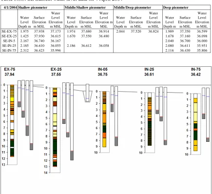
The SE transect (Table 3.8.3) head data, which can be graphically viewed in
Figure 3.8.3, showed that water drains into the perimeter ditch from both sides.
Analyzing the flows in the middle sand layer, there was an indication of water moving
from the exterior to the interior of the bay, but there was only one representative
piezometer inside the bay in this layer. Modeling would help analyzing this part in detail.
In the lower sands, the gradient was from exterior to interior indicating groundwater
Table 3.8.3: SE transect water level data on 4 April 2004
4/1/2004 Shallow piezometer Middle/Shallow piezometer Middle/Deep piezometer Deep piezometer
Water Level Depth m Surface Elevation m MSL Water Level Elevation m MSL Water Level Depth m Surface Elevation m MSL Water Level Elevation m MSL Water Level Depth m Surface Elevation m MSL Water Level Elevation m MSL Water Level Depth m Surface Elevation m MSL Water Level Elevation m MSL SE-EX-75 1.975 37.938 37.173 1.974 37.680 36.914 2.044 37.520 36.824 1.989 37.350 36.599 SE-EX-25 1.425 37.930 36.615 1.670 37.550 36.480 1.678 37.160 36.098
SE-IN-5 2.167 36.740 36.167 2.040 36.700 36.000
SE-IN-25 2.185 36.610 36.055 2.186 36.612 36.058 2.080 36.611 35.951
SE-IN-75 2.312 36.423 35.996 2.116 36.430 35.806
Figure 3.8.3: Hydraulic heads from the SE transect, 4 April 2004. Piezometers and water levels
are shown at relative elevations. Cores at each nest are shown for reference
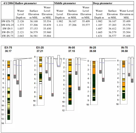
Head data at SW transect on 4 April 2004 (Table 3.8.4) was different in flow
scenario analysis compared to the other transects. The graphical view relative to ground
elevation and soil profile is presented in Figure 3.8.4. In the surface layer, water draining
into the perimeter ditch, and in the middle and deeper layers head gradients suggested
Table 3.8.4: SW transect water level data on 4 April 2004
4/1/2004 Shallow piezometer Middle piezometer Deep piezometer
Water Level Depth m
Surface Elevation
m MSL
Water Level Elevation
m MSL
Water Level Depth m
Surface Elevation
m MSL
Water Level Elevation
m MSL
Water Level Depth m
Surface Elevation
m MSL
Water Level Elevation m
MSL SW-EX-75 2.126 36.168 35.554 1.982 36.167 35.409 1.982 36.167 35.409 SW-EX-25 1.373 37.206 35.839 1.111 37.206 35.577 1.107 37.203 35.570
SW-IN-5 1.037 37.153 35.450 1.687 36.412 35.359
SW-IN-25 2.121 36.579 35.960 1.665 36.579 35.504
SW-IN-75 2.043 36.581 35.884 1.631 36.577 35.468
Figure 3.8.4: Hydraulic heads from the SW transect, 4 April 2004. Piezometers and water levels
Figure 3.8.5: Legend for the Figures 3.8.1-4
3.9 Summary
Data obtained from the cores verified the conceptualization of Juniper Bay
stratigraphy (Figure 3). Five nests of piezometers were installed at each transect with a
water level monitoring system on each nest. Calibration runs for each of the monitoring
units showed very good resolution (1 mm) from the system. Data collection began in late
2003. Installation was completed in early 2004. Over the course of several months, a
number of problems, such as faulty solder joints, were found and corrected.
The preliminary data from this work suggests this resolution will give better
representation of how groundwater is moving at the perimeter of the Bay than the
previously existing hydrologic monitoring system. Figures 3.8.1 to 3.8.4 show the head
data at all transects for the first week of April 2004. Since the resolution is close to
millimeter level, the vertical gradients at the nests can be estimated precisely. This
resolution will also help in precise estimation of hydraulic gradients across the transects.
and groundwater outflow through the SW transect. Groundwater models discussed in
Chapter 4
Modeling and Analysis of Subsurface Flows at the Four
Transects
Stratigraphic information, head data and weather data collected onsite were used
to model subsurface flows on all transects. This chapter discusses the development of the
individual transect, including calibration and validation using Visual MODFLOW.
Analysis of results from model output to determine the direction of flow and the degree
of influence of the perimeter ditch is presented. This chapter addresses the second and
third objectives of the project.
4.1 Model Development
The main objectives of subsurface flow modeling for this project were to:
• Determine the flow directions,
• Determine influence of the perimeter ditch,
• Quantify inflows/outflows, and
• Investigate management options for the ditch.
To achieve this, a two-dimensional, cross-sectional, finite difference groundwater
flow model was developed using Visual MODFLOW, version 4.0 (McDonald and
defining a) the surface extent and thickness of aquifers and confining units, b)
hydrogeologic boundaries which control rate and direction and movement of groundwater
flow, c) hydraulic properties, d) head distribution, and e) groundwater recharge. The
modeling process includes defining input parameters and boundary conditions. The
following sections discuss input parameters and boundary conditions used in this
groundwater modeling.
Input Parameters
The flow domain for each transect was divided into five layers based on the core
descriptions and hydraulic conductivity estimates. These layers represent the surficial
sand layer, first clay layer, a middle sand layer, second clay layer, and a deep sand layer.
The top and bottom elevations of each layer were based on the ground surface elevations
from the survey data. Table 4.1.1 presents top and bottom elevations of the five layers for
the models for each transect. The five layers were assumed to be continuous between
core locations. Although this represents an idealization, it was the best that could be done
with the available field data. This configuration also reduced the complexity of the
model. Effective hydraulic conductivity for each layer was estimated from corresponding
values from five core points in the layer. Piezometric heads were used as inputs to
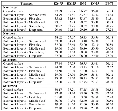
Table 4.1.1: Elevations of five layers for the four transect models, in meters MSL
Transect EX-75 EX-25 IN-5 IN-25 IN-75
Northwest
Ground surface 37.89 36.85 36.72 36.48 36.38
Bottom of layer 1 – Surface sand 34.79 33.81 33.67 32.82 33.34 Bottom of layer 2 – First clay 33.62 32.89 33.67 31.60 31.81 Bottom of layer 3 – Middle sand 33.01 32.28 30.62 30.38 30.29 Bottom of layer 4 – Second clay 30.27 30.76 30.62 30.38 28.76 Bottom of layer 5 – Deep sand 29.66 30.15 29.10 28.86 27.24
Northeast
Ground surface 38.62 37.67 36.43 36.56 36.48
Bottom of layer 1 – Surface sand 33.80 34.70 33.40 32.80 31.50 Bottom of layer 2 – First clay 32.00 32.60 32.00 32.10 30.50 Bottom of layer 3 – Middle sand 29.00 31.00 30.80 30.50 29.00 Bottom of layer 4 – Second clay 29.00 30.50 30.00 30.00 28.50 Bottom of layer 5 – Deep sand 27.00 29.67 28.00 29.00 27.00 Southeast
Ground surface 37.94 37.55 36.75 36.61 36.42
Bottom of layer 1 – Surface sand 34.40 32.00 33.25 33.10 32.42 Bottom of layer 2 – First clay 33.50 31.00 31.00 32.61 31.00 Bottom of layer 3 – Middle sand 29.00 29.50 29.50 31.61 30.42 Bottom of layer 4 – Second clay 28.00 26.50 29.25 28.61 29.00 Bottom of layer 5 – Deep sand 27.00 26.00 27.75 27.61 28.00
Southwest
Ground surface 36.17 37.21 37.15 36.58 36.58
Bottom of layer 1 – Surface sand 32.30 33.70 33.50 33.70 32.50 Bottom of layer 2 – First clay 31.70 31.80 33.20 32.50 32.20 Bottom of layer 3 – Middle sand 30.00 31.80 32.70 31.50 30.50 Bottom of layer 4 – Second clay 29.00 31.20 31.00 30.50 30.20 Bottom of layer 5 – Deep sand 27.70 28.00 29.90 29.80 29.80
Boundary Conditions
Boundary conditions applied to these models are:
1) Known heads at the perimeter ditch at the center of each transect,
2) Known heads (hydrographs from the piezometers) at the EX-75 and IN-75 core
locations to define left and right boundary conditions, respectively.
DRAINMOD (Skaggs, 2004), version 5.1, was run for 2004 data to obtain the percentage
of rainfall that contributed towards runoff.
The weather parameters solar radiation, net radiation, wind speed, soil
temperature, and relative humidity were measured at an on-site weather station. Those
data were used to estimate the ET using the Penman-Monteith Equation. Ref-ET (Allen,
1990) was used to estimate ET. Appendix B provides tables with daily ET and daily
precipitation data for the year 2004.
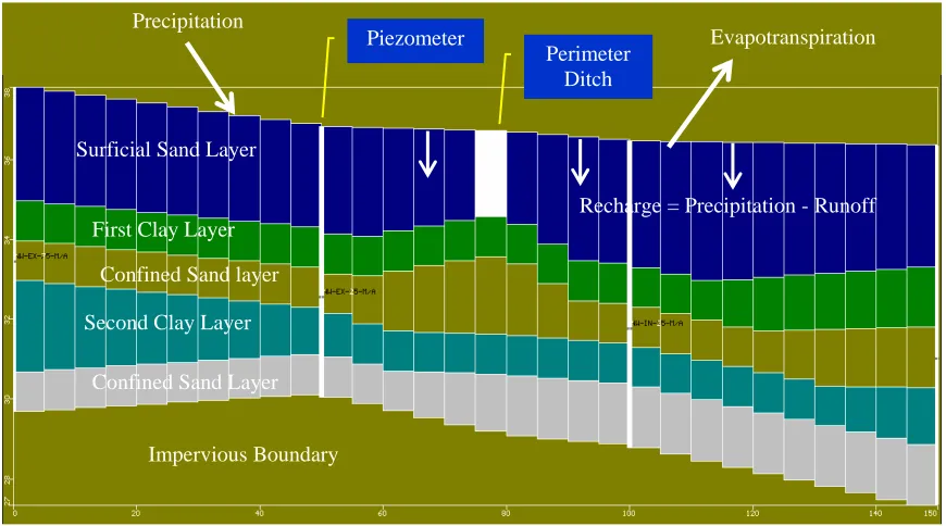
The grid model for the NW transect that was developed using MODFLOW is
shown in Figure 4.1.1. The perimeter ditch is located at the lateral distance of 75 m in the
flow domain. The flow domain on the left side of the ditch represents the exterior of the
bay and the flow domain on the right side of the ditch represents the interior of the bay.
This arrangement is used for all of the models. Given the availability of head data for
only one year (2004), the observed heads from 01 January 2004 to 30 June 2004 were
used for calibration, while the data from 01 July 2004 to 31 December 2004 were used
for testing the model. The following section discusses the calibration process of the
models.
Calibration
To calibrate a groundwater flow model, one needs well-defined calibration targets
and parameters. The calibration targets refer to the observations that are compared with
the calculated values, in this case, the piezometric heads. The calibration parameters are
the parameters that are changed to obtain the best fit between the observed and calculated
as the calibration parameters. Modeling efforts were initially focused on the NW transect,
which is used as an example in the following discussion of calibration and testing.
Figure 4.1.1: Model setup for NW Transect
Initially, the model was run for steady state conditions, and then extended to
transient conditions. Hydraulic conductivity field estimates were available for different
cores in each layer. An effective hydraulic conductivity (Ke) for a layer was calculated
from the lab results as
x x e
x K D K
D
=
∑
(4.1.1)Kx = Ksat of stratum x, and Dx = thickness of stratum x
Effective Ksat for each layer at the NW transect is given in Table 4.1.2. In the
calibration phase, the conductivity values for each layer were varied within the range of
Surficial Sand Layer
First Clay Layer
Confined Sand layer
Second Clay Layer
Confined Sand Layer
Impervious Boundary Precipitation
Evapotranspiration
Recharge = Precipitation - Runoff Perimeter
unconfined and confined layers. For confined layers, specific storage (Ss) was used to
estimate storage volume. For unconfined sand, specific yield (Sy) was used to estimate
storage volume. Specific storage for confined layers was varied from 1E-4 to 1E-9
(Fetter, 1994) and specific yield for the unconfined sand layer was varied from 0.1 to 0.3.
The storage component does not have a significant effect on the model output. Therefore,
the main soil parameter that was used as calibration parameter was hydraulic
conductivity. The correlation coefficients were compared from different runs to find the
parameter set that gave the highest correlation between observed and calculated head
values. The observed correlation coefficient results are shown in Figure 4.1.2. K in the
Figure 4.1.2 refers to set of Kmean values for all five layers.
Table 4.1.2: Effective Saturated Hydraulic Conductivity (m/sec) of different layers
Layer EX-75 EX-25 IN-05 IN-25 IN-75 Kmean