Variable Cant Angle Winglets for Improvement of Aircraft Flight Performance

(1)

V

_{ariable cant angle winglets for improvement of aircraft flight}

performance

A Preprint

Joel E. Guerrero

DICCA

Università degli Studi di Genova Genova, Italy

[email protected]

Marco Sanguineti

DICCA

Kevin Wittkowski

DICCA

June 28, 2019

A

_bstract

Traditional winglets are designed as fixed devices attached at the tips of the wings. The primary purpose of the winglets is to reduce the lift-induced drag, therefore improving aircraft performance and fuel efficiency. However, because winglets are fixed surfaces, they cannot be used to control lift-induced drag reductions or to obtain the largest lift-induced drag reductions at different flight conditions (take-off, climb, cruise, loitering, descent, approach, landing, and so on). In this work, we propose the use of variable cant angle winglets which could potentially allow aircraft to get the best all-around performance (in terms of lift-induced drag reduction), at different flight phases. By using computational fluid dynamics, we study the influence of the winglet cant angle and sweep angle on the performance of a benchmark wing at Mach numbers of 0.3 and 0.8395. The results obtained demonstrate that by adjusting the cant angle, the aerodynamic performance can be improved at different flight conditions.

Keywords Variable cant angle·Winglets·Drag reduction·Lift-induced drag·CFD

Nomenclature

a speed of sound, measured inm/s.

AOA angle-of-attack, measured in degrees (◦).

AOAe f f effective angle-of-attack, measured in degrees (◦).

AOAind induced angle-of-attack, measured in degrees (◦).

CD drag coefficient, nondimensional.

CDmin minimum drag coefficient, nondimensional.

CL lift coefficient, nondimensional.

CL0 lift coefficient at zero angle-of-attack, nondimensional.

CLmax maximum lift coefficient, nondimensional.

CL/CD lift-to-drag ratio, nondimensional.

CP pressure coefficient, nondimensional.

Ma Mach number, nondimensional.

C1 Sutherland model coefficient, 1.458×10−6kg/(m−s−K0.5).

C2 Sutherland model coefficient, 110.4K.

(2)

P∞ freestream pressure, measured inPa.

Re Reynolds number, nondimensional.

Sre f reference surface area, measured inm2.

T local temperature, measured inK.

T∞ freestream temperature, measured inK.

R air specific gas constant, 287.058J/(kg−K).

V local velocity, measured inm/s.

V∞ freestream velocity, measured inm/s.

w downwash, measured inm/s.

y+ viscous wall units, nondimensional.

Greek Symbols

αzl angle-of-attack at zero lift, measured in degrees (◦).

∆CD drag count, 1∆CD=10000×CD, nondimensional.

∂CL/∂AOA slope of the lift curve, measured in 1/◦.

ρ density, measured inkg/m3.

γ air ratio of specific heat, 1.4, nondimensional.

µ dynamic viscosity, measured inkg/(m−s).

κ turbulent kinetic energy, measured inm2/s2.

ω specific dissipation rate, measured in 1/s.

Acronyms

ACARE Advisory Council for Aviation Research in Europe.

CFD Computational Fluid Dynamics.

RANS Reynolds-Averaged Navier-Stokes.

SIMPLE Semi-Implicit Method for Pressure Linked Equations.

κ−ωSST Menter’s Shear Stress Transport turbulence model.

CO2 Carbon Dioxide.

NOx Nitrogen Oxide.

WWSWI Wing-Winglet Shock Wave Interaction.

1 Introduction

Regulatory civil aviation agencies are pushing aircraft manufacturers and operators to improve aircraft efficiency by reducing fuel consumption, cutting carbon dioxideCO2and nitrogen oxideNOxemissions, and lowering the perceived

external noise. One way to help achieve this goal is by using improved and innovative technologies targeting drag reduction, specifically, lift-induced drag reduction. The drag breakdown of a typical transport aircraft shows that the lift-induced drag can amount to as much as 40% of the total drag at cruise conditions and 80-90% of the total drag during take-offand climb conditions(1,2,3,4,5,6,7,8,9). Reducing lift-induced drag is therefore of paramount importance to improve aircraft efficiency.

(3)

A B C D

E F G H

I J K L

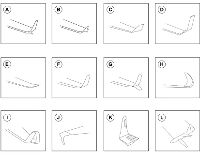
A. Whitcomb Winglet B. Tip Fence

C. Canted Winglet D. Vortex Diffuser E. Raked Tip F. Blended Winglet G. Blended Wplit Winglet H. Sharklet

I. Spiroid Winglet

J. Downward Canted Winglet K. Active Winglet

L. Tip Sails

Figure 1: Different types of winglets and wingtip devices. A) Whitcomb winglet. B) Tip fence. C) Canted winglet. D) Vortex diffuser. E) Raked winglet. F) Blended winglet. G) Blended split winglet. H) Sharklet. I) Spiroid winglet. J) Downward canted winglet. K) Active winglets. L) Tip sails.

wings. But as for the case of wingspan increment, winglets increase bending moments; therefore, it might be necessary to reinforce the wings. From an aerodynamic point of view winglets are desirable; whereas, from a structural standpoint they are detrimental.

Many studies have found that winglets addition can achieve a fuel burn reduction of about 4% to 6%, reduce take-off distance and increase climb rate(1,2,3,4,5,6,7,8,10,11,12,13). Also, as less fuel is burned, emissions are reduced. Winglets can provide up to a 6% reduction inCO2emissions and an 8% reduction inNOxemissions(14,15,16). They also increase

the aftermarket value of the aircraft and add more aesthetic to the airplane design. Winglets are among the most used fuel saving and performance improvement technologies in today’s aviation. The drag reduction gained by adding winglets can be seen as the equivalent decrease in aircraft weight required to carry a payload over a specific distance. A reduction of one drag count in cruise conditions on a subsonic civil transport airplane means about 200 lbs more in payload(17,18,19)(where one drag count is equal to the drag coefficientCDmultiplied by 10000 or∆CD=10000×CD).

As fuel has a large direct operating cost impact in the air transport industry, fuel consumption reduction is translated in more savings, fewer emissions as less fuel is burn, extended operating range and increased payload.

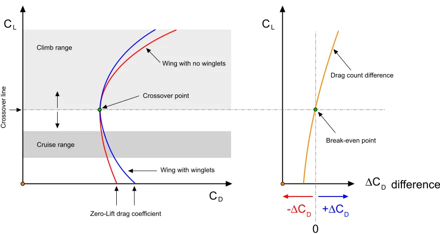
The increment of wings root bending moment is among the few negative effects of winglets. They also increase parasite drag, which is the contribution of skin friction, interference drag, and pressure drag due to separation. Recall that the total drag of an aircraft or a wing is equal to the sum of parasite drag, lift-induced drag and wave drag. Winglets are aerodynamically viable only when the reduction of lift-induced drag is larger than the increment in parasite drag, and this situation is illustrated in figure 2, where we show the drag polars of two hypothetical wings, one wing with no winglets and one wing with winglets installed.

(4)

C

D Crossover point

Wing with winglets

Break-even point Drag count difference

Zero-Lift drag coefficient Cruise range

Crossover line

Climb range

0 difference

+

∆

C

_D

-

∆

C

_D

∆

C

_D

Wing with no winglets

Figure 2: Comparison of drag polars for a wing with no winglets and a wing with winglets installed. In the left image, the light grey area represents the climb range of the wings, and the dark grey area represents the cruise range of the wings. In the right image, we show the drag count difference, where negative∆CDmeans drag increment and positive

∆CDmeans drag reduction. The∆CDdifference is expressed as the drag coefficient∆CDsubtraction between the wing

with winglets and the wing with no winglets.

drag of the wing with no winglets. Conversely, when operating below the crossover line, the total drag of the wing with no winglets is lower than the total drag of the wing with winglets. Therefore, in order to justify the use of winglets in the hypothetical situation illustrated in this figure, we should look at the performance of the wing at a given flight condition. Thus, if the wing were to operate in cruise conditions most of the time (the dark grey region in figure 2), the use of winglets is not justified from a point of view of total drag reduction. On the other hand, if the wing were to operate in climb conditions (the light grey region in figure 2), the use of winglets is justified from an aerodynamic point of view, as the wing generates less drag for a given lift.

As it can be inferred from the previous discussion, the justification of the use of winglets can be based on total drag reduction arguments. So for example and in reference to figure 2, if the crossover point for a given winglet design is located in the cruise region, the use of winglets is justified for that flight condition. The crossover point gives a simple way to measure the total drag reduction trade-offwhen using winglets. However, winglets use can also be justified in the base of other factors, such as wing (or aircraft) performance at a different altitude. For example, if we climb to a higher altitude where the air is lighter, the wing in discussion would have to flight at a higher angle-of-attack (AOA) that might fall in the light grey region illustrated in figure 2; therefore, the use of winglets is justified based on total drag reduction arguments. As it can be guessed, there might exist different winglet configurations that might shift the crossover point below (or above) what is illustrated in figure 2.

During the 1970s oil crisis, commercial airlines and aircraft manufacturers explored many ways to reduce fuel consumption as a consequence of the high cost of jet fuel. It was not until the late 1970s that R.T. Whitcomb, an engineer at NASA Langley Research Center, pioneered the concept of the modern winglet we see in today’s aircraft, as a mean to reduce cruise drag and improve aircraft performance(11,12). Whitcomb’s work(12), marks the first time a winglet was seriously considered for large and heavy aircraft. Since Whitcomb breakthrough work on winglets, many variations have been designed (as depicted in figure 1), but all of them have been designed as passive or fixed devices attached at the wingtips. That is, the angle between the wing plane and the winglet plane (or cant angle) does not change; therefore, they are designed to deliver lift-induced drag reduction at a single design configuration, which might not be the best winglet configuration to generate the largest lift-induced drag reduction during different flight phases.

(5)

DOWNWASH UPWASH

LH WINGTIP VORTEX

RH WINGTIP VORTEX

VORTEX CORE

RH WINGTIP

VORTEX

LH WINGTIP

VORTEX

HIGH PRESSURE (BOTTOM SURFACE)

LOW PRESSURE (TOP SURFACE)

TRAILING EDGE VORTICES TRAILING EDGE VORTICES

A

B

Figure 3: (A) Illustration of lift generation due to pressure imbalance and its associated trailing edge and wingtip vortices. (B) Illustration of wingtip vortices rotation and the associated downwash and upwash.

at different flight conditions to get the best lift-induced drag reduction for the given flight phase; or it can be kept in the vertical position while in ground so that it reduces wingspan while meeting gate and runaway clearance; or it can act as a load alleviation mechanism where in the case of gusts or strong sideslip velocities, the winglet can adjust itself, so it reduces the bending moment on the wing and the device itself. Similar solutions have been already proposed, but most of them focused on the use of shape memory alloy materials(20,21,22,23,24,25)_{, foldable wings during}

ground operations(26,27,28,29,30)_{, load alleviation mechanisms}(31,32,33,34,35)_{, complaint surfaces}(25,36,37,38,39,40)_{, and rotating}

systems for mitigating wingtip vortices(41,42,43,44,45); but just a few of them have addressed variable cant angle winglets for drag reduction while flying(41,47,48,49)_.

The wing used in this study is the Onera M6 wing(50,51), with a variable cant angle winglet installed, and we conduct the study at two Mach numbers (Ma=0.3 andMa=0.8395) and different angle-of-attack values. Thus, we aim at covering take-off, climb, approach, descent, and cruise conditions. The concept presented hereafter represents an innovative approach that the authors’ hope holds potential to realize the goal of drag reduction to directly address the global challenge of improving aircraft fuel efficiency and reduce pollutant emissions, as highlighted in the reports ACARE - European aeronautics: A vision for 2020(52)and ACARE - Flightpath 2050: Europe’s vision for aviation(53).

2 A brief review of lift-induced drag and its reduction using winglets

Finite span wings generate lift due to the pressure imbalance between the bottom surface (high pressure) and the top surface (low pressure), as illustrated in figure 3. However, as a byproduct of this pressure differential, cross flow components of the velocity are generated (which are unavoidable but can be mitigated). The higher pressure air under the wing flows around the wingtips and tries to displace the lower pressure air on the top of the wing. This motion generates a trailing edge vortex, and at the wingtips, where the flow curls, large vortices are formed. This flow around the wingtips is sketched in figure 3. These structures are referred to as wingtip vortices, and high velocities and low pressure exist at their cores. These vortices (trailing edge vortices and wingtip vortices), produce a downward flow in

the neighborhood of the wing, known as the downwash and is denoted with the letterwin figure 4. The downwash

interacts with the free-stream velocity to induce a local relative wind deflected downward in the vicinity of each airfoil section of the wing, as sketched in figure 4. The presence of the downwash reduces the angle-of-attack that each section of the wing effectively sees, and it creates a component of drag, the lift-induced drag, as it will be explained hereafter.

In figure 4, the angle between the airfoil chord line and the direction of the undisturbed free-streamV∞is the

angle-of-attackAOA, which we will call geometricAOA. In this figure, the local relative wind is inclined downward due to the downwashw, which gives rise to the induced angle-of-attack orAOAind. Therefore, theAOAactually seen by

the local airfoil section is the angle between the chord line and the local relative wind, or the effective angle-of-attack AOAe f f defined asAOAe f f =AOA−AOAind. Even if the wind is at a geometricAOA, the local airfoil section always

sees a smaller angle. This variation of the localAOAis more pronounced towards the wingtips, where the downwash is stronger. Recall that the lift force is perpendicular to the local relative wind. In the presence of the downwash, the local lift vector is inclined by the angleAOAind, as shown in figure 4. As it can be seen in this figure, there is a component

(6)

= INDUCED ANGLE OF ATTACK = EFFECTIVE ANGLE OF ATTACK

=

-LOCAL RELA_{TIVE WIND}

CHORD LINE OF THE LOCAL AIRFOIL

SECTION OF THE WING

LIFT COMPONENT LIFT FORCE VECTOR

ACTS NORMAL TO THE LOCAL RELATIVE WIND

W

UNDISTURBED FREE-STREAM V

_h

AOA

ind AOA

V

_h

eff AOA eff

AOAind

AOA

eff

AOA AOA AOAind

ind AOA

ind

AOA

Figure 4: Illustration of lift-induced drag due to downwash.

A scenario similar to that of the downwash of the wing can be found at the winglets. Consider a section of the winglet as illustrated in figure 5. At the winglets the tip vortex is rolling up, therefore is generating a sidewash which induces a velocity component pointing towards the fuselage. As for the wings, the induced velocity component will create a local relative wind that will tilt the local lift vector, and for well-designed winglets the force component parallel to the undisturbed free-stream will point forward, therefore generating thrust (in analogy to sails in a sail boat). As a consequence, the thrust generated by the winglet counteracts any skin-friction and interference drag produced by the winglet itself. A similar analysis can be done for winglets bent downwards where the induced velocity is pointing outward, but operational requirements and ground clearances favor winglets bent upwards(54).

Well-designed winglets will reduce the trailing vortex strength (hence the wingtip vortex) and the average wing downwash by modifying the pressure distribution (which is related to the spanwise lift distribution), and shifting the shed vorticity away from the wing plane (as sketched in figure 6). They will also counteract the skin friction and interference drag of the winglets by generating a thrust force induced by the sidewash(2,12,54)_{. All this translate into less}

total drag due to the reduction of lift-induced drag and the parasite drag generated by the winglet.

3 Wing model, computational domain, boundary conditions, and initial conditions

The wing model used in this study is the Onera M6, as described in references(50,51)_{. To model the variable cant angle}

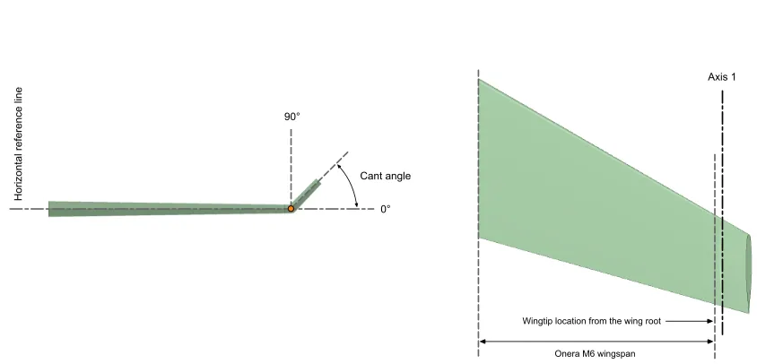
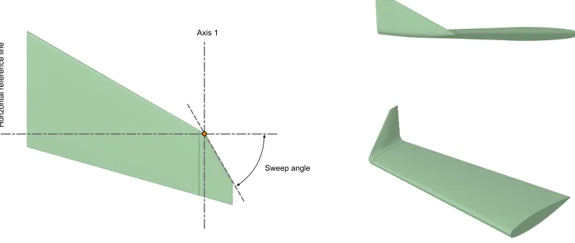
winglet, an extension to the baseline Onera M6 wing was added (as shown in figure 7). Then, the cant angle is modeled by adding a small curvature radius at the wingtip join with the winglet, in such a way as to guarantee a smooth transition between the wing and the winglet (as illustrated in figure 8). The winglet span used in this study corresponds to a 20% of the wingspan of the baseline wing. This value was chosen on the basis of previous studies(1,6,12,55,56,57,58), where the authors suggest the use of winglet span values between 10% to 20% of the wingspan. Additionally, we also studied the influence of the winglet sweep angle on the aerodynamic performance of the wing, where the sweep angle is defined as illustrated in figure 9. In table 1, we report the cant angles, sweep angles, and angle-of-attack values used in this study. As a guideline, in table 2 we report the wetted area of each wing used. Lastly, in table 3, we report the values of the relative wingspan reduction in reference to the wing with winglet at cant angle 0◦.

(7)

UNDISTURBED FREE-STREAM V

h

LOCAL RELA

TIVE WIND

INBOARD LIFT COMPONENT

LIFT FORCE VECT

OR ACTS NORMAL

TO THE LOCAL RELA_{TIVE WIND}

FOR

W

ARD LIFT COMPONENT

INDUCED VELOCITY

INDUCED ANGLE

WINGLET CHORD LINE OF THE

LOCAL AIRFOIL SECTION OF THE WINGLET

FUSELAGE

Figure 5: Illustration of forces generated at the winglets. Notice that for well-designed winglets there is a generation of thrust that counteracts skin friction and interference drag effects.

High pressure Low pressure

Figure 6: Wingtip vortices. Left image: wing with no winglet, in this wing a larger and stronger vortex is shed, resulting in more lift-induced drag. Right image: wing with winglet, in this wing a narrower and less intense vortex is shed, resulting in lower lift-induced drag. Also, the vortex is shifted away from the wing plane occurring in lower downwash.

Table 1: Design space explored in this study. All the angles are defined in degrees.

Winglet cant angle 0, 15, 45, 80

Winglet sweep angle 30, 45, 60

Angle-of-attack atMa=0.3 0-20 (spaced at intervals of 2)

(8)

Onera M6 wingspan

Winglet extension (20% wingspan)

Figure 7: Wing and winglet extension. The winglet span used in this study corresponds to a 20% of the wing span of the original Onera M6 wing.

Cant angle 90°

0°

Axis 1

Horizontal reference line

Onera M6 wingspan Wingtip location from the wing root

(9)

Sweep angle

Horizontal reference line

Axis 1

Figure 9: Left image: winglet sweep angle definition. Right image: winglet geometry corresponding to a cant angle of 80◦and a sweep angle of 60◦.

14 R 12

FAR-FIELD

FAR-FIELD FAR-FIELD

OUTLET

SYMMETR

Y

FAR-FIELD

(0 0 0) (0 0 0)

NO-SLIP WALL

R 12

CENTER LINE

Y

X

Y

Z INFLOW

AOA

Figure 10: Computational domain and boundary conditions (all dimensions are in meters). The illustration is not to scale.

boundaries. The wing was modeled as a no-slip wall, where we used continuous wall function boundary conditions for the turbulence variables. In all cases, the average distance from the wing surface to the first cell center offthe surface is approximately four viscous wall units (y+≈4 ).

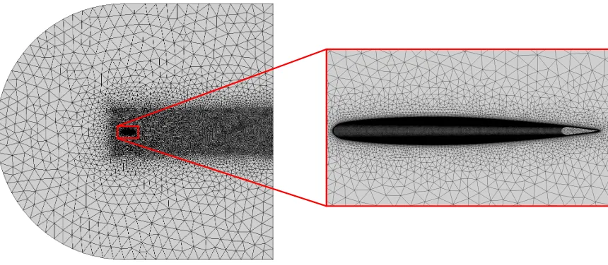
A hybrid mesh was used for all the simulations, with prismatic cells close to the wing surface and tetrahedral and polyhedral cells for the rest of the domain. Also, in the vicinity of the wing and wake region, we added a refinement region with uniform cell size (as illustrated in figure 11). A typical mesh is made up of approximately 3.6 to 4.1 million cells, depending on the cant and sweep angle.

The lift forceLand drag forceDare calculated by integrating the pressure and wall-shear stresses over the wing surface; then, the lift coefficientCLand drag coefficientCDare computed as follows:

CL=

L 0.5×ρ×V2

∞×Sre f

and CD=

D 0.5×ρ×V2

∞×Sre f

(10)

Figure 11: Domain mesh. The mesh is visualized in the symmetry plane and wing surface.

Table 2: Wetted area of each wing used in this study.

Wing Reference area (m2)

Baseline wing (original Onera M6 wing) 1.5952

Wing with winglet - Winglet sweep angle 30◦ _1.7881

Wing with winglet - Winglet sweep angle 45◦ 1.7694

Wing with winglet - Winglet sweep angle 60◦ 1.7388

Finally, theAOAwas changed by adjusting the incidence angle value of the inlet velocity, and all forces were computed in the reference system aligned with the inlet velocity. All the computations were initialized using free-stream values and the incoming flow is characterized by a turbulence intensity value equal to 5.0%. All the turbulence variables were initialized following the guidelines given in references(59,60,61)_.

4 Numerical method and validation

The compressible Reynolds-Averaged Navier-Stokes (RANS) equations are solved by using the finite volume solver Ansys Fluent(62)_{. The cell-centered values of the variables are interpolated at the face locations using a second-order}

centered difference scheme for the diffusive terms. The convective terms are discretized by means of the second-order upwind scheme(63)_{. For computing the gradients at cell-centers, the least squares cell-based reconstruction method is}

used. In order to prevent spurious oscillations, a multi-dimensional gradient limiter is used(64)_{. The pressure-velocity}

coupling is achieved by means of the SIMPLE algorithm(65,66), where we used the default under-relaxation parameters. As the solution takes place in collocated meshes, the Rhie-Chow interpolation scheme is used to prevent the pressure checkerboard instability. For turbulence modeling, theκ−ωSST model is used(59,60,61)_{. The turbulence quantities,}

namely, turbulent kinetic energyκand specific dissipation rateω, are discretized using the same scheme as for the convective terms.

Before proceeding to the parametric study, we assessed the accuracy of the numerical scheme and mesh resolution used. In this validation study, we compare the numerical solution outcome against the data of the physical experiments at the

Table 3: Relative wingspan reduction in reference to the wing with winglet at cant angle 0◦.

Wing Wingspan reduction (%)

Wing with winglet at cant angle 0◦ –

Wing with winglet at cant angle 15◦ ≈0.5

Wing with winglet at cant angle 45◦ _≈₄_.₀

Wing with winglet at cant angle 80◦ ≈11.2

(11)

Table 4: Comparison ofCLandCDobtained with different solvers (data taken from reference(51)). The comparison is

done for meshes with similar cell count.

Solver - Mesh type CL CD

CFL3D - Structured mesh 0.2661 0.0173

USM3D - Tetrahedral mesh 0.2649 0.0186

FUN3D - Prismatic mesh 0.2659 0.0172

Current solution - Hybrid mesh (tetrahedra+polyhedra+prisms) 0.2597 0.0188

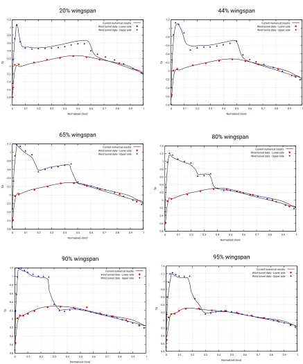
same operating conditions described by Schmitt and Charpin(50), that is, Reynolds numberRe=11.72×106, Mach numberMa=0.8395, and angle-of-attack equal to 3.06◦_.

In figure 12, we plot the pressure coefficientC p=(p−p∞)/(0.5ρV∞2) values obtained from the numerical simulations

against the experimental values at different wingspan locations. As it can be seen, the numerical solution shows a similar trend to theC pdistribution obtained in the wind tunnel experiments. Additionally, in table 4 we compare theCL

andCDvalues against the values obtained using different CFD solvers(51). In this table, we can evidence a fairly good

match among all solvers, even if the meshes and solution methods are different. In this validation study, the reference area used forCLandCDcomputations is equal to 0.7532m2, as described in reference(50).

As a side note, the turbulence model used in reference(51)_{was the Spalart-Allmaras whereas in this study we used the}

κ−ωSST. Additionally, we did not model the rounded wingtip as described in references(50,51), so these two factors might represent a source of uncertainty, which however we deem to be negligible for the purposes of this study. Based on the results presented, we can state that the selected numerical scheme, turbulence model, and mesh resolution are adequate to resolve the physics involved.

Finally, during this study air was modeled using the equation of state for ideal gases, and the dynamic viscosity was computed using the Sutherland model. It is worth mentioning that the original Onera M6 wing report(50), does not give specific details about the working conditions; therefore, we assumed air at sea-level and at 300◦ K. The temperature was determined by using an iterative procedure so thatReandMaconditions are matched, together with the equation of statep=ρRT, the speed of sound relationshipa= √γRT, and the Sutherland dynamic viscosity equation µ=(C1T3/2)/(T +C2) (whereT is the temperature given in degrees Kelvin, andC1andC2are the coefficients of the

Sutherland model). While it is difficult to determine if the operating conditions used in the simulations correspond to the same conditions of the wind tunnel experiments, the assumptions taken in this study appear to be justified given the good agreement between the physical experiments and the numerical simulations.

5 Numerical results and discussion

In this section, we discuss the results of the aerodynamic performance of the wing with variable cant angle winglet in reference to the baseline wing (original Onera M6 wing). An extensive campaign of simulations was carried out, as per the design space listed in table 1. For all cases, the reference area used forCLandCDcomputations is equal to 1.0m2.

The computations were carried out in parallel using 16 cores, and each simulation took approximately 4 to 6 hours to convergence to a level where the forces showed either a non-oscillatory behavior or a periodic behavior.

5.1 Aerodynamic performance at high Mach number –Ma=0.8395

Hereafter, we discuss the results at Mach number equal to 0.8395, which might corresponds to a typical velocity encountered at cruise conditions on subsonic civil transport aircraft. We exploreAOAvalues up to 10◦_{, which correspond}

to the values ofAOAthat might be encountered during cruise and change of cruise level on medium and long-range subsonic transport aircraft.

Let us use the drag polars plotted in figures 13-15 to study the influence of the winglet cant angle and sweep angle on the aerodynamic performance of the wing. By looking at these figures, we can notice a strong influence of the sweep angle on the drag polars, that is, as we increase the sweep angle, the drag polar curves are shifted upward, and this trend contributes to an improvement of the aerodynamic performance,i.e., for the same lift coefficient less drag is produced. For instance, in figure 13 (winglet sweep angle 30◦_{) we can see that when the winglet cant angle is equal to 80}◦_the

overall performance of the wing is worse than that of the baseline wing, or in other words, for a given value ofCL

the wing with winglet will produce more drag. However, as we increase the sweep angle, the drag polar is slightly shifted upwards, so eventually, the wing with winglet will produce less drag for a givenCLvalue when compared to

the baseline wing. This situation is illustrated in figures 14 and 15, where for example, for a value ofCL=0.3 all the

(12)

-1.2 -1 -0.8 -0.6 -0.4 -0.2 0 0.2 0.4 0.6 0.8 1

0 0.1 0.2 0.3 0.4 0.5 0.6 0.7 0.8 0.9 1

Cp

Normalized chord

20% wingspan

Current numerical results Wind tunnel data - Lower side Wind tunnel data - Upper side

-1.2 -1 -0.8 -0.6 -0.4 -0.2 0 0.2 0.4 0.6 0.8

0 0.1 0.2 0.3 0.4 0.5 0.6 0.7 0.8 0.9 1

Cp

Normalized chord

44% wingspan

-1.2 -1 -0.8 -0.6 -0.4 -0.2 0 0.2 0.4 0.6 0.8

0 0.1 0.2 0.3 0.4 0.5 0.6 0.7 0.8 0.9 1

Cp

Normalized chord

65% wingspan

-1.4 -1.2 -1 -0.8 -0.6 -0.4 -0.2 0 0.2 0.4 0.6 0.8

0 0.1 0.2 0.3 0.4 0.5 0.6 0.7 0.8 0.9 1

Cp

Normalized chord

80% wingspan

-1.2 -1 -0.8 -0.6 -0.4 -0.2 0 0.2 0.4 0.6 0.8

0 0.1 0.2 0.3 0.4 0.5 0.6 0.7 0.8 0.9 1

Cp

Normalized chord

90% wingspan

-1.4 -1.2 -1 -0.8 -0.6 -0.4 -0.2 0 0.2 0.4 0.6 0.8

0 0.1 0.2 0.3 0.4 0.5 0.6 0.7 0.8 0.9 1

Cp

Normalized chord

95% wingspan

(13)

-0.05 0.00 0.05 0.10 0.15 0.20 0.25 0.30 0.35 0.40 0.45 0.50

0.00 0.01 0.02 0.03 0.04 0.05 0.06 0.07 0.08 0.09 0.10 0.11

Lift

coefficien

t C

L

Drag coefficient CD

Base wing

Cant angle 0° - Sweep angle 30° Cant angle 15° - Sweep angle 30° Cant angle 45° - Sweep angle 30° Cant angle 80° - Sweep angle 30°

Figure 13: Drag polar at Mach number 0.8395, sweep angle 30◦and different values of cant angle.

-0.05 0.00 0.05 0.10 0.15 0.20 0.25 0.30 0.35 0.40 0.45 0.50

0.00 0.01 0.02 0.03 0.04 0.05 0.06 0.07 0.08 0.09 0.10 0.11

Lift

coefficien

t C

L

Drag coefficient CD

Base wing

(14)

-0.05 0.00 0.05 0.10 0.15 0.20 0.25 0.30 0.35 0.40

0.00 0.01 0.02 0.03 0.04 0.05 0.06 0.07 0.08 0.09 0.10 0.11

Lift

coefficien

t C

L

Drag coefficient CD

Base wing

Figure 15: Drag polar at Mach number 0.8395, sweep angle 60◦_{and di}_ff_{erent values of cant angle}

Table 5: Wing-winglet wave drag ratio atAOA2◦_.

Winglet sweep angle (◦) Winglet cant angle (◦) Wing-winglet wave drag ratio

30 80 1.0

60 80 0.8515

60 45 0.8195

60 15 0.8250

60 0 0.8481

Baseline wing 0.7773

The effect of the sweep angle on the aerodynamic performance can be explained by the fact that at higher sweep angles less skin friction drag and interference drag is produced. Another factor that contributes to the drag reduction at high Mach number is the impact of the winglet sweep angle on the wave drag. This particular wing is known to generate a shock wave system on the wing surface; this shock wave interacts with the winglet (as depicted in figures 16 and 17), therefore increasing the wave drag.

In figure 16, we illustrate the wing-winglet shock wave interaction (WWSWI) for two different winglet sweep angles and a cant angle of 80◦_{, where the shock wave region was computed using the criterion of Lovely and Haimes}(67)_.

In this figure, we can observe that for larger sweep angles the shock wave intensity is reduced. Hence, as for wings designed for high-speed, the sweep-back angle have a positive effect in reducing the wave drag of the winglets. In figure 17, we show the WWSWI but this time for a sweep angle of 60◦_{and three di}_ff_{erent cant angles. In this figure, we can}

observe that for large cant angle values the WWSWI is stronger, thus the wave drag is larger. It is worth mentioning that the WWSWI might also cause additional detrimental phenomena, such as boundary layer separation and buffeting.

In table 5, we quantify the wave drag ratio for five representative configurations atAOA2◦_{. In this table, the wave}

drag ratio is calculated as the ratio of the wave drag of the given wing-winglet configuration and the wave drag of the configuration with a winglet sweep angle of 30◦_{and a cant angle of 80}◦_{(the arrangement that generates the largest}

wave drag and parasite drag). In all cases, the wave drag was computed using the drag decomposition method described by Destarac and van der Vooren(68). From these quantitative results, we can see the influence of the cant angle on the wave drag, that is, as we decrease the cant angle the wave drag decreases. We can also note that as we increase the winglet sweep angle, the wave drag is reduced. It is worth noting that the increment of the wave drag due to the winglet addition is almost proportional to the wingspan increment of the baseline wing (20%).

(15)

Wing-Winglet shock wave interaction

Figure 16: Shock wave system forAOA2◦, winglet cant angle 80◦and two different values of winglet sweep angle. The left image corresponds to a winglet sweep angle of 30◦_{and the right image to a sweep angle of 60}◦_{. The shock}

wave region was computed using the criterion of Lovely and Haimes(67).

Wing-Winglet shock wave interaction

Figure 17: Shock wave system forAOA2◦_{, winglet sweep angle 60}◦_{, and di}_ff_{erent values of winglet cant angle. The}

left image corresponds to a winglet cant angle of 80◦_{, the middle image to a cant angle of 45}◦_{, and the right image to a}

(16)

superior parasite drag generated by the winglet at high cant angles and the reduction of the pressure differential towards the wingtips.

To understand the reason of the pressure differential reduction, let us take a look at figure 18, where the pressure coefficient on the wing surface is displayed for a configuration with winglet sweep angle 60◦_{and four cant angles.}

In this figure, we can observe that as we increase the cant angle, the winglet will work as a wall that will reduce the pressure differential between the bottom and top surfaces of the wing. This reduction of the pressure differential, which is stronger towards the wingtip, is responsible for the decrement of the maximumCLand the slope of the lift curve. As

we reduce the cant angle, the reduction in the pressure differential is lessened, therefore the maximum lift increases, as it can be confirmed in figure 19. The winglet effect of reduction of the pressure differential also affects drag, as it can be seen in figure 20. But in this case, the reduction of the pressure differential has a positive impact by reducing the drag and the intensity of the wingtip vortices.

Let us quantify the minimum drag coefficientCDmin in the drag polar plots depicted in figures 13-15. Hereafter, we compute theCDminpercentage reduction (or increment) in reference to the baseline wing. For the wing with winglet sweep angle 30◦_{(figure 13), the configuration with cant angle 80}◦_increases_C

Dminby approximately 30%, for cant angle 45◦_the_C

Dminis increased by≈10%, for cant angle 15

◦_the_C

Dmin is increased by≈7.0%, and for cant angle 0

◦_the

CDminis increased by≈4.0%. If we now take a look at figure 14 (wing with winglet sweep angle 45

◦_{), the situation is}

slightly different. In this figure, the configurations with cant angles 0◦_{and 15}◦_increase_C

Dmin by about 4.0%, for a cant angle of 45◦theCDminis increased≈5.0%, and theCDmin of the wing with winglet cant angle 80

◦_{is approximately 7.0%}

larger. Finally, in figure 15 (wing with winglet sweep angle 60◦), theCDminof the wing with winglet cant angle 80

◦_is

approximately 2.5% larger, whereas theCDmin for the other cant angles is increased by about 1.0%. These results clearly indicate that large cant angle values generate more parasite drag (possibly due to strong interference effects).

In the previous discussion, the reduction ofCDmin as the winglet sweep angle is increased, can be attributed to the fact that at higher sweep angles less skin friction drag and interference drag is produced. Also, the addition of the sweep angle to the winglet and the sidewash generated by the flow in the surroundings of the winglet, might modify the inboard lift force generated by the winglet (as depicted in figure 5), which contributes to reducing (or increasing) theCDmin. It is also important to note that in figure 15, none of the configurations with winglet installed have a strong detrimental crossover point. In all cases plotted in this figure and forAOAless than 2◦_{, the wings with winglet generate}

little less drag, or the difference is negligible respect to the baseline wing. ForAOAlarger than 2◦_{the di}_ff_{erence in}_C D

for the sameCLis more evident.

To make a comprehensive treatment of how the variable cant angle winglets could improve the wing aerodynamic performance, let us compute theCDat threeCLtargets, namely, 0.1, 0.2, and 0.35. In this hypothetical situation, theCL

targets could correspond to cruise conditions or 0.1<CL<0.2 (which corresponds to the maximumCL/CDratio) and

cruise climb conditions orCL=0.35 (which approximately corresponds to the maximumC2L/CDratio and is on the

limit of the linear regime of the lift curve). These results are summarized in tables 6-8 and as it can be seen, for cruise conditions (0.1<CL<0.2) the largest drag reduction is obtained at cant angles between 0◦and 45◦, this suggest that

the winglets could be adjusted in flight according to fuel consumption. For cruise climb (CL=0.35), the best results are

obtained at a cant angle value of 15◦. However, values up to 80◦are also acceptable as they produce less drag for the sameCL.

These results show how winglets reduce the drag by artificially increasing the wingspan. The relative wingspan reduction is shown in table 3, by cross-referencing these values with the results shown in tables 6-8, it can be seen that as we reduce the wingspan (by increasing the winglet cant angle), the aerodynamic performance is improved in reference to the baseline wing. In general, for cant angle 80◦the gains in drag reduction are not the same to those achieved by merely extending the wingspan by an amount equal to the winglet span (equivalent to a winglet configuration with cant angle 0◦), but approximately half that amount. For the other cant angle values (45◦and 15◦) the drag reduction is about the same amount or even larger. In addition, increasing the winglet cant angle does not add the extra wing root bending moment that would be encountered if the wingspan were simply increased by the span of the winglet, and this is a desirable benefit from the structural point of view.

For completeness, in figure 21 we plot the drag polars for fixed cant angles and different sweep angles. In this figure, we can better highlight the influence of the sweep angle on the aerodynamic performance. It is clear that as we increase the sweep angle the crossover point is shifted downwards, up to the point that the performance of the wing with winglets is better in the whole envelope of the drag polar. For the case with cant angle equal to 45◦_{, the crossover point is located}

(17)

Top surface

Bottom surface

Winglet cant angle 0°

Figure 18: Pressure coefficient on the wing surface at Mach number 0.8395. Winglet sweep angle equal to 60◦_and

(18)

-0.05 0.00 0.05 0.10 0.15 0.20 0.25 0.30 0.35 0.40 0.45

0.00 1.00 2.00 3.00 4.00 5.00 6.00 7.00 8.00 9.00 10.00

Lift

coefficien

t C

L

AOA (°)

Base wing

Figure 19: Lift coefficient versus angle-of-attack at Mach number 0.8395, sweep angle 60◦and different values of cant angle.

0.00 0.01 0.02 0.03 0.04 0.05 0.06 0.07 0.08 0.09 0.10 0.11

0.00 1.00 2.00 3.00 4.00 5.00 6.00 7.00 8.00 9.00 10.00

D

rag coefficien

t C

D

AOA (°)

Base wing

(19)

Table 6:CDand drag reduction percentage for a targetCLequal to 0.1 at Mach number 0.8395. The drag reduction

percentage was computed with respect to the baseline wing, where positive values indicate drag reduction.

Winglet cant angle Winglet sweep angle CD Drag reduction (%)

0◦ ₆₀◦ _0.010246 _≈₀_.₈

15◦ 60◦ 0.010276 ≈0.5

45◦ ₆₀◦ _0.010501 _{≈ −}₁_.₅

80◦ ₆₀◦ _0.010530 _{≈ −}₁_.₉

0◦ ₆₀◦ _0.015319 _≈₉_.₅

15◦ 60◦ 0.015319 ≈9.5

45◦ 60◦ 0.015829 ≈6.5

80◦ ₆₀◦ _0.016085 _≈₅_.₀

45◦_{and 60}◦_{, the crossover point is located approximately between 2}◦_{and 3}◦_of_{AOA, and for a sweep angle of 30}◦_the

polars intersect at largeCLvalues (worst case scenario).

From the previous discussion, we found that the sweep angle has a strong influence on the aerodynamic performance and, the best performance is obtained for a winglet sweep angle equal to 60◦; therefore, for the remainder of this section we will focus our attention on the wing with a winglet sweep angle of 60◦_.

In figure 19, the behavior of the lift coefficient is displayed as a function of theAOA. We can observe in this figure that up to anAOAof 4◦_{, the lift curves show a linear behavior. We can also note that the slope of the lift curve is almost}

the same for the cases with cant angles between 0◦_{and 45}◦₍_∂_C

L/∂AOA≈0.075 per degree). For the case with cant

angle equal to 80◦the slope is lower (∂CL/∂AOA≈0.068 per degree), but still is higher than that of the baseline wing

(∂CL/∂AOA≈0.064 per degree). In this figure, the maximum lift coefficientCLmaxis increased by as much as 10.5% for a cant angle of 0◦_{, approximately 9.1% for a cant angle of 15}◦_{, about 4.2% for a cant angle of 15}◦_{, and for a cant}

angle of 80◦the value ofCLmaxis reduced approximately 1%. The reduction ofCLmax(as the cant angle is increased), is related to the reduction of the pressure differential towards the wingtip, as explained previously. Again, these results correlate well with the fact that winglets artificially increase the effective span of the wing; therefore, they have a direct impact on the lift behavior. Lastly, the use of the variable cant angle winglet does not appear to have any negative effect on the stall behavior, and all cases exhibit gentle stall characteristics.

It is important to mention that computingCLmaxand capturing the stall pattern in CFD is a difficult task, however, as we do not expect that the wing will operate at values close toCLmaxin cruise conditions, uncertainties in the computation of CLmaxcan be tolerated.

It is also interesting to mention that even though the wing airfoil section is symmetric, the lift at zeroAOAorCL0is

not zero for large cant angles of the winglet device. For the winglet with a cant angle of 45◦CL0 ≈0.0055, and for

a winglet cant angle of 80◦CL0 ≈0.0065. Although these values are low, they have the effect of introducing a small

negative zero-lift angle orαzl, which is in the order of−0.1◦.

In figure 20, we plot the behavior of the drag coefficient as a function of theAOA. In this figure, we can observe that forAOAvalues ranging from 0◦_{to 2}◦_{all the winglet configurations generate almost the same drag. Then, as we}

pass byAOA4◦higher cant angles (45◦and 80◦) translate in less drag for the sameAOAvalue. As the wing profile is symmetric, the minimum dragCDmin is attained atAOA0

◦_{, and the use of the winglet does not appear to shift the}

horizontal location ofCDmin.

0◦ 60◦ 0.036936 ≈11.2

15◦ ₆₀◦ _0.035148 _≈₁₅_.₄

45◦ 60◦ 0.038042 ≈8.6

(20)

-0.05 0.00 0.05 0.10 0.15 0.20 0.25 0.30 0.35

0.00 0.01 0.02 0.03 0.04 0.05 0.06 0.07 0.08 0.09 0.10 0.11 0.12

Lift

coefficien

t C

L

Drag coefficient CD

Base wing Cant angle 0° - Sweep angle 30° Cant angle 0° - Sweep angle 45° Cant angle 0° - Sweep angle 60°

-0.05 0.00 0.05 0.10 0.15 0.20 0.25 0.30 0.35 0.40 0.45 0.50

0.00 0.01 0.02 0.03 0.04 0.05 0.06 0.07 0.08 0.09 0.10 0.11 0.12

Lift

coefficien

t C

L

Drag coefficient CD

-0.05 0.00 0.05 0.10 0.15 0.20 0.25 0.30 0.35

0.00 0.01 0.02 0.03 0.04 0.05 0.06 0.07 0.08 0.09 0.10 0.11 0.12

Lift

coefficien

t C

L

Drag coefficient CD

-0.05 0.00 0.05 0.10 0.15 0.20 0.25 0.30 0.35 0.40 0.45 0.50

0.00 0.01 0.02 0.03 0.04 0.05 0.06 0.07 0.08 0.09 0.10 0.11 0.12

Lift

coefficien

t C

L

Drag coefficient CD

Figure 21: Drag polar at Mach number 0.8395. Each image corresponds to a fix cant angle and three different values of sweep angle.

The behavior of the lift-to-drag ratio (CL/CD) as a function of theAOAis plotted in figure 22. In this figure, it is

found thatCL/CDincreases very rapidly up to about 2◦, at this point the maximumCL/CDvalue is reached, then,

CL/CDgradually drops mainly because drag increases more rapidly than lift. For winglet cant angles of 0◦and 15◦

the maximumCL/CDis increased by approximately 12.0% in reference to the baseline wing, for a cant angle of 45◦

the maximumCL/CDis increased≈8.8%, and for a cant angle of 80◦the maximumCL/CDis increased≈4.8%. The

main point of interest about theCL/CDcurve is the fact that this ratio is maximum at anAOAof about 2◦for all the

configurations, that is, the use of the variable cant angle winglet does not change theAOAat which the maximum CL/CDoccurs. It is at thisAOAthat the wings will generate as muchCLas possible with a smallCDproduction.

From the results presented, it is clear that there is not a single winglet configuration that can give the best all-around drag reduction at everyAOA. It was also clear that the winglet configuration with a sweep angle equal to 60◦_{gave the}

best results for different cant angle values. The results also show thatCLmaxand the slope of the lift curves decreases as the winglet cant angle is increased, but the aerodynamic performance still is better or similar to that of the baseline wing. This suggests that the proposed variable cant angle winglet can also be used as a load alleviation mechanism. Thus, in the case of strong gusts or turbulence, the cant angle can be increased in order to reduce the lift force, hence decreasing the root bending moment.

5.2 Aerodynamic performance at low Mach number –Ma=0.3

Hereupon, we discuss the results at Mach number equal to 0.3, which might well correspond to the velocities encountered at take-off, climb, descent and approach flight conditions on subsonic civil transport aircraft. We exploreAOAvalues up to 20◦, which correspond to the large values ofAOAthat could be encountered during take-off. It is also important to point out that the trends we will present in this section are very similar to those presented in section 5.1, but as the Mach number is relative low, there are neither wave drag contributions nor compressibility effects.

(21)

-2.00 0.00 2.00 4.00 6.00 8.00 10.00 12.00 14.00

0.00 1.00 2.00 3.00 4.00 5.00 6.00 7.00 8.00 9.00 10.00 CL

/CD

Ra

tio

AOA (°)

Base wing

Figure 22: Lift-to-drag ratio versus angle-of-attack at Mach number 0.8395, sweep angle 60◦and different values of cant angle.

-0.05 0.00 0.05 0.10 0.15 0.20 0.25 0.30 0.35 0.40 0.45 0.50 0.55 0.60

0.00 0.02 0.04 0.06 0.08 0.10 0.12 0.14 0.16 0.18 0.20 0.22

Lift

coefficien

t C

L

Drag coefficient CD

Base wing

(22)

-0.05 0.00 0.05 0.10 0.15 0.20 0.25 0.30 0.35 0.40 0.45 0.50 0.55 0.60

0.00 0.02 0.04 0.06 0.08 0.10 0.12 0.14 0.16 0.18 0.20 0.22

Lift

coefficien

t C

L

Drag coefficient CD

Base wing

Figure 24: Drag polar at Mach number 0.3, sweep angle 45◦and different values of cant angle

-0.05 0.00 0.05 0.10 0.15 0.20 0.25 0.30 0.35 0.40 0.45 0.50 0.55 0.60

0.00 0.02 0.04 0.06 0.08 0.10 0.12 0.14 0.16 0.18 0.20 0.22

Lift

coefficien

t C

L

Drag coefficient CD

Base wing

(23)

Table 9:CDand drag reduction percentage for a targetCL equal to 0.25 at Mach number 0.3. The drag reduction

0◦ ₆₀◦ _0.014742 _≈₁₀_.₀

15◦ 60◦ 0.014820 ≈9.5

45◦ ₆₀◦ _0.015622 _≈₄_.₆

80◦ ₆₀◦ _0.015961 _≈₂_.₅

0◦ 60◦ 0.027495 ≈19.0

15◦ ₆₀◦ _0.027784 _≈₁₈_.₄

45◦ 60◦ 0.029152 ≈14.5

80◦ 60◦ 0.030366 ≈10.1

The reduction ofCLseen in figures 23-25 as the cant angle is increased, and that ofCLmaxand the slope of the lift curve (figure 26), are due to the pressure differential reduction towards the wingtips, as already explained in section 5.1. In figure 27, we plot the pressure coefficient on the wing surface for three configurations. In this figure, we can observe that for large winglet cant angles the pressure differential is reduced towards the wingtips, and this behavior is responsible for the decrement of the maximumCLand the reduction of the slope of the lift curve seen in figure 26.

As for theCDminconcerns, for all cases shown in figures 23-25,CDmin is increased with respect to the baseline wing by approximately 4.0%.

In tables 9-11, we present theCDfor threeCL targets in the linear regime of the lift curves. The values studied

correspond toCLequal to 0.25 (approximately theCLvalue corresponding to anAOAof 4◦where the maximumCL/CD

happens), and two high lift cases (CLequal to 0.4 and 0.45). From the results summarized in these tables, we can

deduce that as the can angle is increased the gains in drag reduction are shortened, and the largest reductions of drag are obtained for cant angles between 0◦and 15◦. In the results presented in table 11, the gains in drag reduction are lessened because we are close toCLmax, and almost in the non-linear regime of the lift curves, hence, the slopes of the lift curves are lower.

In figure 26, we plot the lift coefficient as a function of theAOAfor a sweep angle equal to 60◦_{. The curves depicted in}

this figure show a linear behavior up to approximately 10◦, then,CLmax is reached, and the wings stall. It is noteworthy that the stall behavior of all the cases is similar. In this figure,CLmax is increased in reference to the baseline wing for all winglet cant angle configurations. For a cant angle of 0◦_{the maximum}_C

Lis increased by as much as 13.0%,

approximately 10.0% for a winglet cant angle of 15◦, for a cant angle of 45◦by approximately 7.0%, and for a cant angle of 80◦_,_C

Lmaxis increased by approximately 1.0%. The slope of the lift curves is almost the same for the cases with cant angles between 0◦_{and 45}◦₍_∂_C

L/∂AOA≈0.053 per degree). For the case with a cant angle equal to 80◦the

slope is∂CL/∂AOA≈0.049 per degree. Lastly, the slope of the baseline wing is∂CL/∂AOA≈0.045 per degree.

In figure 28, we plot the behavior of the drag coefficient as a function of theAOA. In this figure, we can observe that for AOAvalues ranging from 0◦to 6◦all the winglet configurations generate almost the same drag. Then, as we pass by AOA8◦_{higher cant angles (45}◦_{and 80}◦_{) translate in less drag for the same}_AOA_{value. From the results presented,}

the largest drag reduction at highAOAis obtained with winglets at cant angle equal to 80◦; however, this winglet configuration greatly reduces the maximumCLwhich is not desirable since at low Mach number largeAOAare needed

to reach the required lift, especially during take-off.

0◦ 60◦ 0.036458 ≈16.7

15◦ ₆₀◦ _0.036273 _≈₁₇_.₁

45◦ 60◦ 0.038001 ≈13.1

(24)

-0.10 0.00 0.10 0.20 0.30 0.40 0.50

0.00 2.00 4.00 6.00 8.00 10.00 12.00 14.00 16.00 18.00 20.00

Lift

coefficien

t C

L

AOA (°)

Base wing

Figure 26: Lift coefficient versus angle-of-attack at Mach number 0.3, sweep angle 60◦_{and di}_ff_{erent values of cant}

angle.

The behavior ofCL/CD as a function of theAOA is plotted in figure 29, where it can be seen that the maximum

value ofCL/CDoccurs at 4◦for all cases. For winglet cant angles of 0◦and 15◦the maximumCL/CDis increased

by approximately 10.5% in reference to the baseline wing, for a cant angle of 45◦_{the maximum}_C

L/CDis increased ≈5.0%, and for a cant angle of 80◦the maximumCL/CDis increased≈3.0%.

Finally, as for the case atMa=0.8395, the winglet configuration with a sweep angle equal to 60◦_{gave the best results}

for different cant angle values.

5.3 Comparison of the aerodynamic performance at low and high Mach numbers

To better understand the impact of high Mach number and compressibility effects on the aerodynamic performance, in figures 30 and 31 we plot the results atMa=0.3 andMa=0.8395, together. In figure 30, we plot the drag polars for the two design Mach numbers, as it can be seen, compressibility plays an important role on the aerodynamic performance. At high Mach numbers, compressibility affectsCLandCDdetrimentally. First, it reducesCLmax, and secondly, it increases the drag for a givenCL, especially for highAOA. This behavior stems from the alteration of the

pressure distribution due to shock waves forming on the wing surface. It is interesting to highlight that at high Mach number and lowAOA, the wing with winglets seem to work better than at low Mach number and lowAOA, asCDminis slightly reduced in reference to the baseline wing.

The behavior ofCLas a function ofAOAis plotted in figure 31, where we can identify two important aspects of the lift

curves at high Mach number. First, the reduction ofCLmax, and second, the increment of the lift curves slope, which in practice means that a smallerAOAis required to generate a givenCL. However, more drag is produced due to

compressibility effects (shock waves). It is also important to highlight that the stall characteristics for both Mach numbers are similar.

5.4 Winglet settings during flight operations

(25)

Top surface

Bottom surface

Baseline wing

Figure 27: Pressure coefficient on the wing surface at Mach number 0.3. Winglet sweep angle equal to 60◦_{and wing}

(26)

0.00 0.02 0.04 0.06 0.08 0.10 0.12 0.14 0.16 0.18 0.20 0.22

0.00 2.00 4.00 6.00 8.00 10.00 12.00 14.00 16.00 18.00 20.00

D

rag coefficien

t C

D

AOA (°) Base wing

Figure 28: Drag coefficient versus angle-of-attack at Mach number 0.3, sweep angle 60◦and different values of cant angle.

0.00 2.00 4.00 6.00 8.00 10.00 12.00 14.00 16.00 18.00

0.00 2.00 4.00 6.00 8.00 10.00 12.00 14.00 16.00 18.00 20.00

CL /CD

R

atio

AOA (°)

Base wing

(27)

-0.05 0.00 0.05 0.10 0.15 0.20 0.25 0.30 0.35 0.40 0.45 0.50 0.55 0.60

0.00 0.02 0.04 0.06 0.08 0.10 0.12 0.14 0.16 0.18 0.20 0.22

Lift

coefficien

t C

L

Drag coefficient CD

Ma=0.8395 - Base wing

Ma=0.8395 - Cant angle 0° - Sweep angle 60°

Ma=0.8395 - Cant angle 15° - Sweep angle 60° Ma=0.8395 - Cant angle 45° - Sweep angle 60°

Ma = 0.3 - Base wing

Figure 30: Drag polar for a winglet sweep angle of 60◦and different cant angles. The results atMa=0.8395 are plotted using continuous lines and those atMa=0.3 are plotted with dashed lines.

-0.05 0.00 0.05 0.10 0.15 0.20 0.25 0.30 0.35 0.40 0.45 0.50 0.55 0.60

0.00 2.00 4.00 6.00 8.00 10.00 12.00 14.00 16.00 18.00 20.00

Lift

coefficien

t C

L

AOA (°)

Ma=0.8395 - Base wing

Ma=0.8395 - Cant angle 15° - Sweep angle 60° Ma=0.8395 - Cant angle 45° - Sweep angle 60°

Ma = 0.3 - Base wing

(28)

1 2

3 4

5

6

0 7

45°- 80° 15°

15°

45°

80° 80°

3. Cruise

4. Change of cruise level 5. Cruise

6. Descent-Approach-Landing 7. Taxiing to gate

Winglet cant angle

Figure 32: Winglet configuration during different flight phases.

were chosen in base of the improvements in the aerodynamic performance with respect to the baseline wing. Hereafter, we summarized the best settings according to the given flight phase:

• During ground operations, it is suggested to use a cant angle of 80◦_{in order to reduce the wingspan and meet}

gate clearance requirements.

• At take-offand initial climb (where compressibility effects are not strong), it is recommended to use a winglet cant angle of 45◦_{. This configuration has a higher lift-slope and generates less drag for a target lift. However, a}

winglet cant angle of 15◦can also be used, this selection criterion can be based on weather conditions, take-off weight, or other operational requirements (such as climb rate).

• At cruise (high Mach number), it is recommended to use a cant angle of 15◦. This setting will give the largest drag reduction for a given lift, with the exception for the case of cant angle equal to 0◦_{. This selection is}

justified mainly because it generates less wing bending moments.

• At cruise level change, it is recommended to use a cant angle of 45◦, but a value of 15◦is also acceptable. These configurations have large lift-slope and generate less drag for a target lift.

• During descent, it is recommended to use a cant angle of 45◦_{. In our analysis, we did not favor configurations}

with a cant angle value equal to 80◦because they reduce the maximum lift coefficient and the slope of the lift curve.

• After landing and when taxiing to the gate, it is suggested to use a cant angle of 80◦_{in order to the reduce}

wingspan and meet gate clearance requirements.

The device studied can also be used as a load alleviation mechanism. So in case of strong gusts or turbulence, the cant angle can be increased to 80◦_{reducing in this way the maximum lift and the slope of the lift curve, therefore reducing}

the wing bending moments, and this might be particularly helpful during descent and landing with adverse weather conditions.

It is worth mentioning that the proposed winglet configurations show similar characteristics to those of fixed winglets already in use in civil transport aircraft. For example, the cant angle configuration of 15◦is very similar to the raked winglet, and the cant angle configuration of 45◦_{is close to the blended and canted winglets (refer to figure 1).}

6 Conclusions and perspectives

In this manuscript, we have studied the use of variable cant angle winglets which could potentially allow aircraft to get the best all-around performance in terms of drag reduction over different flight phases. While the wing studied does not correspond to an actual wing used in civil transport aircraft, the insight gathered can be used to set the guidelines for the design of variable cant angle winglets and the adjustment of their cant angle during flight.

During this work, we considered high and low Mach number values (0.8395 and 0.3, respectively) and different

(29)

adverse effects on the stall behavior and theAOAat whichCLmaxandCDminoccurs. It also worth noting that at high cant angle values (80◦_{), the maximum lift coe}_ffi_{cient and the slope of the lift curve is reduced (but their values are still larger}

than the values of the baseline wing); therefore, the proposed winglet could potentially be used as a load alleviation system.

Furthermore, it was also found that large winglet sweep angle values have a positive impact on the aerodynamic performance improvements gained by using the proposed winglet. The improvement due to sweep angle is mainly due to a combination of reduced parasite drag, decreased wave drag at high Mach number, and the effect of the inboard lift force generated by the winglet.

In summary, the following benefits have been found:

• Increased lift curve slope.

• Increased maximum lift.

• Increased lift-to-drag ratio.

• No negative effects on stall behavior due to lift production enhancement.

• For the same Mach number, theAOAforCLmaxand maximumCL/CDremains almost invariable.

• Crossover point atAOAvalues below 2◦−3◦, and as low as 0◦. As a consequence, total drag reduction for the same lift above the crossover point.

• The increase of the winglet cant angle does not add the extra wing root bending moment that would be

encountered if the wingspan were simply increased by the span of the winglet.

On the other side, the following shortcomings have been found:

• Increased parasite drag.

• Increased wave drag at high Mach number and cant angle 80◦.

• Noticeable reduction ofCLmaxand lift curve slope for a winglet cant angle of 80

◦_.

• Increased weight due to the device itself.

• The addition of the winglet will require a structural study in order to support the local forces and bending moments at the winglet junction.

• A new structural study of the wing to meet the new bending moments and flutter and fatigue requirements due to the addition of the winglet.

It is clear that to obtain the best trade-offbetween benefits and shortcomings, a multi-disciplinary design optimization study should be conducted, together with the use of more realistic wing geometries and additional winglet design variables, such as toe-angle, taper ratio, and span. We also envisage conducting a flight performance study using more realistic wing-winglet configurations. Nevertheless, the concept studied in this manuscript represents an innovative approach that might help in addressing the challenge of improving aircraft fuel efficiency, reduce pollutant emissions, and lowering the perceived external noise.

References

[1] Torenbeek, E. Advanced Aircraft Design: Conceptual Design, Analysis and Optimization of Subsonic Civil

Airplanes, 2013, Wiley.

[2] Kroo, I. Drag due to lift: Concepts for prediction and reduction,Annual Review of Fluid Mechanics, 2001,33, (1),

pp 587–617.

[3] Kroo, I. Nonplanar wing concepts for increased aircraft efficiency, in: VKI lecture series on Innovative

Configura-tions and Advanced Concepts for Future Civil Aircraft, 2005.

[4] Bertin, J. J. and Cummings, R. M. Aerodynamics for Engineers, 2013, Pearson.

[5] J_obe, C. E. Prediction of aerodynamic drag, Technical Report AFWAL-TM-884-203, Air Force Wright Aeronauti-cal Laboratories, Wright-Patterson Air Force, Ohio, United States, 1984.

[6] NATO AGARD. Aircraft drag prediction and reduction, Technical Report AGARD report 723, NATO, 1985.

[7] Filippone, A. Data and performances of selected aircraft and rotorcraft,Progress in Aerospace Sciences, 2000,36,