Multi – objective Analysis and Parametric Estimation of Machining Force Delamination and Surface Quality in Milling Process on FRP composite through Statistical Linked DSA

(1)

2089 | P a g e 

Multi – objective Analysis and Parametric Estimation of

Machining Force Delamination and Surface Quality in

Milling Process on FRP composite through Statistical

Linked DSA

D.Ramalingam

1

*, R.RinuKaarthikeyen

1

, S.Muthu

2

, V.Sankar

3

1

Principal, James college of Engineering and Technology, Nagercoil, (India)

1

Research Associate, Manager – Engineering, TCMPFL, Chennai, (India)

2

Principal, Adithya Institute of Technology, Coimbatore, (India)

3

Professor, Nehru Institute of Engineering and Technology, Coimbatore, (India)

ABSTRACT

Milling process is one among the common traditional metal cutting operations mainly to trim down to the size, shape and required surface quality. At the same time during milling operations on composite materials, the commonly named damage delamination is one of the inevitable issue which are mainly depend on the input machining parameters. In this attempt the optimization of machining parameters referring to the surface roughness and delamination during milling on Viapal VUP 9731 GFRP composite material, is analyzed through Differential Search Algorithm and estimated the optimal combinations of such parameters. The objective is to lay down a path for reference according to the requirement of the product end quality. Initially algorithm is executed in MATLAB to iterate the values and the effectiveness of simulation is analyzed individually by means MSE. Subsequently the regression relationship is taken as the conditional approach for further simulation. On confirming the outcome found to be tuned with the earlier results further forecasting of delamination factor, surface roughness for various combination of machining parameters is executedwith step up number of iterations.

KEYWORDS :

Milling, Viapal 9731 frp composite, Surface finish, Machining Force, Delamination, DSA,

Hybrid, Optimisation, Minitab, MATLAB

.

1 INTRODUCTION

(2)

outcome is associated with the input cutting parameters. During the machining operations on FRP composites the machining forces significantly influence and make the major impact on the surface quality such as delamination and surface roughness. In this study, the experiment conducted on Viapal VUP 9731 frp composites by [1] is taken and the optimsation method through DSA is applied to identify the improved combination of machining parameters.

ABBREVIATIONS AND SYMBOLS USED

FRP Fiber Reinforced Plastic N Newton

v Cutting speed, m/min DSA Differential Search Algorithm

f Feed, mm/rev Reg Regression

F Machining force, N R-sq R - square statistical value

Df Delamination factor R-sq (adj) R - square adjusted statistical value

Ra Surface Roughness R-sq (pred) R - square predicted statistical value

II

LITERATURE

REVIEW

(3)

2091 | P a g e

fluids also on hole quality and declared that the dry-drilled holes resulted in poorer surface finish than holes produced with cutting fluid application along with main cutting parameters. Ramulu et al. [11] have stated that the surface roughness and delamination is the characteristic that could influence the dimensional precision, production costs and the performance of end product and because for these reasons there has been research and development with the objective of optimising cutting conditions, to obtain a desired machinability.

III

EXPERIMENTAL

OBSERVATION

[1]

On the Viapal VUP 9731 reinforced with 65% of glass fiber unsaturated polyester hand lay-up material, which posses the material properties as listed in the Table 3.1milling process experiment has performed to analyse the machining force during machining and the milling induced damage namely delamination factor, surface quality after machining by J Paulo Davim et al [1] with the statistical tool analysis (ANOVA).

Table 3.1 Properties of Viapal VUP 9731 frp[1]

Property Value

Flexural strength (DIN EN 63) 480 N/mm2

Tensile modulus (DIN 53457) 26,470 N/mm2

Tensile strength (DIN EN 61) 480 N/mm2

Compressive strength (DIN 53454) 196 N/mm2

Tensile elongation (DIN EN 61) 1.7 %

Impact resistance (DIN 53453) 150 190 kJ/m2

Martens temperature (DIN 53458) 200 0C

Thermal conductivity (DIN 52612) 0.15 0.22 W/m0C

The specimen wasmade up on the hand lay-up discs with 22 mm thickness and machining operations carried out with a 5 mm diameter cemented carbide end mill on the „„VCE500 MIKRON‟‟ machining center with 11 kW spindle power and a maximum spindle speed of 7500 rpm. With L9 Taguchi array as the plan of DOE by assigning cutting velocity (v); feed rate (F) as machining input parameters to evaluate the outputs variables - machining force on the workpiece (Fm), delamination factor (Df), surface roughness (Ra). The three states of machining variables

chosen are listed in Table 3.2.

Table 3.2 Input cutting variables

Milling parameters S1 S2 S3

Cutting speed, (v); m/min 47 79 110

Feed, (f); mm/rev 0.04 0.08 0.12

(4)

500 microscope used to measure the damage caused on the specimen composite material. The obtained observation outcome of the experiments was arranged in the Table 3.3.

Table 3.3 Experimental observation [1]

Exp

v

f

F

D

f

R

a

1

47

0.04

21.67

1.030

1.42

2

47

0.08

38.96

1.041

1.69

3

47

0.12

54.19

1.064

1.86

4

79

0.04

19.85

1.045

1.24

5

79

0.08

33.40

1.057

1.43

6

79

0.12

47.35

1.086

1.75

7

110

0.04

15.54

1.057

1.02

8

110

0.08

23.32

1.069

1.28

9

110

0.12

32.89

1.097

1.48 IV STATISTICAL PROJECTIONS

On evaluating the regression relationship between the parameters and Best Subsets Regression analysis in Minitab the point noted through Table 4.1 the second regression analysis of F versus v, f shows the statistically significant relationship between the variables at the 95% confidence level and the model summary reveals the R-sq value as 99.73% which is significant and model fit. Also the Durbin-Watson test the statistic value is greater than 0.05, shows that there is no indication of serial autocorrelation. In the Df versus v, f analysis the R-sq value is 99.79%

&Regression Analysis of Ra versus v, f statistical significance relationship between the variables at the 95% confidence level exists as the R-sq value as 97.13 % which confirms the significance.

Table 4.1 Regression Model summary

Parameter Regression S R-sq R-sq(adj)

R-sq(pred) Durbin - Watson

F Second order 1.10613 99.73% 99.29% 96.76% 1.70277

Df Second order 0.0015853 99.79% 99.45% 97.60% 1.71057

Ra Second order 0.0779463 97.13% 92.34% 77.69% 3.33973

Based on the model summary the regression equations framed for all the three output parameters are:

 Machining force = - (8.94) + (0.416 x machining speed) + (556.5 x feed) – (0.002573 x machining speed2) + (14 x feed2) – (3.004 x machining speed x feed)

(5)

2093 | P a g e

 Surface roughness = (0.543) + (0.01208 x machining speed) + (16.05 x feed) – (0.000119 x machining speed2) – (65.6 x feed2) + (0.0041 x machining speed x feed)

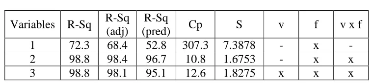
Table 4.2 Best Subsets Regression: F versus v, f, v x f

Variables R-Sq

R-Sq

(adj)

R-Sq

(pred)

Cp

S

v

f

v x f

1

72.3

68.4

52.8

307.3 7.3878

-

x

-

2

98.8

98.4

96.7

10.8 1.6753

-

x

3

98.8

98.1

95.1

12.6 1.8275

x

The best subset analysis results posted through the Tables 4.2; 4.3; 4.4 confirms the contribution of tool feed as higher influence on F, Df and Ra over the cutting speed.

Table 4.3 Best Subsets Regression: D

f

versus v, f, v x f

Variables R-Sq

R-Sq

(adj)

R-Sq

(pred)

Cp

S

v

f

2

v x f

1

92.5

91.4

87.8 103.9 0.0062532

-

x

2

98.7

98.3

97.0

15.4 0.0027794

x

-

x

-

3

99.1

98.6

97.1

11.7 0.0025290

x

-

Table 4.4 Best Subsets Regression: Ra versus v, f, v x f

Variables R-Sq

R-Sq

(adj)

R-Sq

(pred)

Cp

S

v

f

v

2

1

52.2

45.4

22.7

44.8 0.20800

-

x

-

2

91.7

89.0

87.2

5.6 0.093566

-

x

2

89.2

85.6

82.6

8.2 0.10669

x

-

3

93.6

89.8

81.7

5.6 0.089870

x

Hence the second order regression relationship is considered for the application towards further evaluation.

V

OPTIMIZATION

TECHNIQUES

Differential Search Algorithm optimisation method is chosen and applied in this attempt in MATLAB to appraise the influence of the cutting velocity, tool feed on to the work material towards the resultant parameters Delamination factor and Surface roughness and to estimate the optimal parameters combination for the quality outcome through the optimization. Though Elman Back Propagation domain in MATLAB the DSA programme as follows.

(6)

case 1,

% BIJECTIVE DSA (B-DSA) (i.e., go-to-rnd DSA);

% philosophy: evolve the superorganism (i.e.,population) towards to "permuted-superorganism (i.e., random directions)"

direction=superorganism(randperm(size_of_superorganism),:); msg=' B-DSA'; case 2,

% SURJECTIVE DSA (S-DSA) (i.e., go-to-good DSA)

% philosophy: evolve the superorganism (i.e.,population) towards to "some of the random top-best" solutions ind=ones(size_of_superorganism,1);

[null_,B]=sort(fit_superorganism);

for i=1:size_of_superorganism, ind(i)=B(randi(ceil(rand*size_of_superorganism),1)); end; direction=superorganism(ind,:); msg=' S-DSA';

case 3,

% ELITIST DSA #1 (E1-DSA) (i.e., go-to-best DSA)

% philosophy: evolve the superorganism (i.e.,population) towards to "one of the random top-best" solution [null,jind]=sort(fit_superorganism); ibest=jind(ceil(rand*size_of_superorganism)); msg='E1-DSA'; direction=repmat(superorganism(ibest,:),[size_of_superorganism 1]);

case 4,

% ELITIST DSA #2 (E2-DSA) (i.e., go-to-best DSA)

% philosophy: evolve the superorganism (i.e.,population) towards to "the best" solution [null_,ibest]=min(fit_superorganism); msg='E2-DSA';

direction=repmat(superorganism(ibest,:),[size_of_superorganism 1]); end

(7)

2095 | P a g e

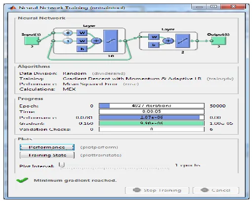
Figure 5.1 Data training progress of 50000 iterations

Upon the comparison, it is evident that the performance of the DSA is in the close tolerance the algorithm is coded to the execution in the Gradient Descent with Momentum & Adaptive Learning. The performance indicator is the mean square error. Based on the objectives, the coding was developed towards optimization, i.e. surface roughness to the minimum value as the objective functions. Initially the simulation is trained for 50000 iterations. Mean squared error in computation is found as 0.3640 with the compiling time 74.1137.

Figure 5.2 Flow chart of Regression hybridization with DSA

The regression relationship equations generated by the Minitab is fed into the programme for the closeness in resulting the simulation (MSE = 0.29382) and 19.28 % improvement in error reduction is noticed. The relevant flow of hybridization is shown through the Figure 5.2. With this the values for the step up periodical (15 intervals) between the parameter selection is chosen for subsequent simulation. The step up value for such computation is chosen as (47 : 4.2 : 110) for the speed parameter and (0.04 : 0.00533 : 0.12) for the feed parameters. The computed values through this hybrid approach are given in the Table 5.1.

Experimental data

Regression Modeling

DSA in MATLAB

Hybridization of Regression relationship as

condition in MATLAB

Simulated Results

Simulation and confirmation of

(8)

Table 5.1 F, Df, Ra for v = 47, 51.2 and 55.4 m / min.

Feed v = 47 m /min v = 51.2 m /min v = 55.4 m /min

F Df Ra F Df Ra F Df Ra

0.040 21.670 1.030 1.420 21.741 1.002 1.477 21.834 1.006 1.446

0.045 23.784 1.028 1.447 23.786 1.010 1.452 23.292 1.012 1.449

0.051 26.002 1.057 1.723 26.051 1.045 1.664 26.008 1.040 1.645

0.056 28.229 1.044 1.700 28.205 1.055 1.686 28.096 1.055 1.657

0.061 30.451 1.037 1.722 30.361 1.055 1.704 30.185 1.059 1.686

0.067 32.674 1.024 1.751 33.872 1.031 1.730 34.405 1.037 1.705

0.072 34.157 1.034 1.757 35.332 1.039 1.740 35.575 1.039 1.721

0.077 41.025 1.030 1.784 38.891 1.030 1.762 38.482 1.036 1.741

0.083 43.909 1.041 1.794 41.983 1.050 1.776 41.204 1.048 1.757

0.088 44.672 1.038 1.809 44.044 1.047 1.790 43.441 1.050 1.770

0.093 45.387 1.044 1.823 45.412 1.050 1.806 45.014 1.053 1.787

0.099 46.764 1.046 1.833 46.752 1.050 1.816 46.362 1.054 1.798

0.104 48.836 1.056 1.846 48.427 1.067 1.829 47.896 1.061 1.812

0.109 51.236 1.052 1.855 50.562 1.058 1.839 49.912 1.062 1.822

0.115 53.671 1.059 1.865 52.986 1.062 1.850 52.319 1.064 1.834

0.120 56.268 1.062 1.873 55.586 1.066 1.859 54.919 1.072 1.843

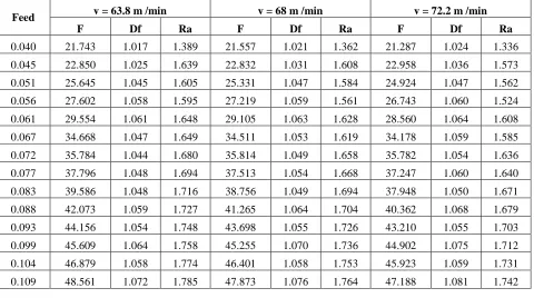
Table 5.2 F, Df, Ra for v = 63.8, 68 and 72.2 m / min.

Feed v = 63.8 m /min v = 68 m /min v = 72.2 m /min

0.040 21.743 1.017 1.389 21.557 1.021 1.362 21.287 1.024 1.336

0.045 22.850 1.025 1.639 22.832 1.031 1.608 22.958 1.036 1.573

0.051 25.645 1.045 1.605 25.331 1.047 1.584 24.924 1.047 1.562

0.056 27.602 1.058 1.595 27.219 1.059 1.561 26.743 1.060 1.524

0.061 29.554 1.061 1.648 29.105 1.063 1.628 28.560 1.064 1.608

0.067 34.668 1.047 1.649 34.511 1.053 1.619 34.178 1.059 1.585

0.072 35.784 1.044 1.680 35.814 1.049 1.658 35.782 1.054 1.636

0.077 37.796 1.048 1.694 37.513 1.054 1.668 37.247 1.060 1.640

0.083 39.586 1.048 1.716 38.756 1.049 1.694 37.948 1.050 1.671

0.088 42.073 1.059 1.727 41.265 1.064 1.704 40.362 1.068 1.679

0.093 44.156 1.054 1.748 43.698 1.055 1.726 43.210 1.055 1.703

0.099 45.609 1.064 1.758 45.255 1.070 1.736 44.902 1.075 1.712

0.104 46.879 1.058 1.774 46.401 1.058 1.753 45.923 1.059 1.731

(9)

2097 | P a g e

0.115 50.806 1.067 1.797 49.954 1.068 1.777 49.063 1.068 1.755

0.120 53.363 1.083 1.808 52.442 1.087 1.788 51.409 1.090 1.766

Table 5.3 F, Df, Ra for v = 76.4, 80.6 and 84.8 m / min.

Feed v = 76.4 m /min v = 80.6m /min v = 84.8 m /min

0.040 20.923 1.025 1.311 20.472 1.026 1.287 19.923 1.027 1.263

0.045 23.248 1.039 1.534 23.727 1.043 1.490 24.393 1.046 1.441

0.051 24.423 1.046 1.540 23.836 1.045 1.516 23.155 1.045 1.489

0.056 26.177 1.061 1.485 25.519 1.062 1.441 24.774 1.063 1.392

0.061 27.927 1.065 1.586 27.207 1.065 1.563 26.391 1.065 1.537

0.067 33.705 1.064 1.549 33.136 1.068 1.509 28.012 1.072 1.464

0.072 35.680 1.058 1.612 30.577 1.062 1.587 29.632 1.065 1.559

0.077 36.986 1.066 1.610 36.718 1.071 1.577 31.252 1.076 1.540

0.083 37.187 1.054 1.646 36.483 1.057 1.619 35.839 1.061 1.589

0.088 39.387 1.073 1.652 38.390 1.077 1.623 37.429 1.082 1.592

0.093 42.678 1.056 1.678 42.104 1.058 1.651 41.495 1.061 1.621

0.099 44.531 1.080 1.688 44.119 1.084 1.661 37.740 1.088 1.632

0.104 45.411 1.060 1.707 44.817 1.062 1.680 44.099 1.064 1.651

0.109 46.514 1.085 1.718 45.832 1.089 1.692 45.110 1.093 1.664

0.115 48.189 1.068 1.732 47.411 1.068 1.706 46.792 1.069 1.678

0.120 50.289 1.093 1.743 49.149 1.095 1.718 48.082 1.098 1.691

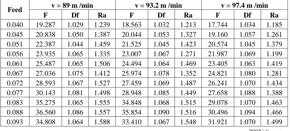
Table 5.4 F, Df, Ra for v = 89, 93.2 and 97.4 m / min.

Feed

v = 89 m /min

v = 93.2 m /min

v = 97.4 m /min

F

Df

Ra

F

Df

Ra

F

Df

Ra

(10)

0.099

36.366

1.091

1.600

34.898

1.095

1.563

33.341

1.098

1.519

0.104

43.250

1.066

1.619

36.387

1.069

1.581

34.763

1.071

1.536

0.109

44.320

1.096

1.633

43.482

1.099

1.598

36.189

1.101

1.556

0.115

46.342

1.071

1.646

39.369

1.073

1.610

37.609

1.075

1.568

0.120

47.149

1.100

1.660

46.347

1.102

1.625

39.034

1.104

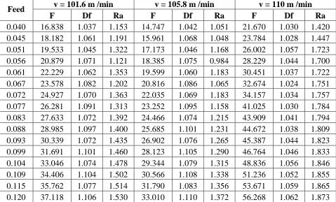
1.583 Table 5.5 F, Df, Ra for v = 101.6, 105.8 and 110 m / min.

Feed

v = 101.6 m /min

v = 105.8 m /min

v = 110 m /min

F

Df

Ra

F

Df

Ra

F

Df

Ra

(11)

2099 | P a g e

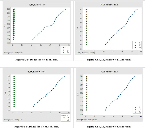
Figure 5.3 F, Df, Ra for v = 47 m / min. Figure 5.4 F, Df, Ra for v = 51.2 m / min.

(12)

Figure 5.5 F, Df, Ra for v = 68 m / min. Figure 5.4 F, Df, Ra for v = 72.2 m / min.

(13)

2101 | P a g e

Figure 5.5 F, Df, Ra for v = 84.8 m / min. Figure 5.4 F, Df, Ra for v = 110 m / min.

VI RESULTS AND CONCLUSIONS

The experimental data set well fit in the second order statistical regression model. The regression relationship linked Differential Search Algorithm converges with minimal off set in simulation in terms of MSE. The contribution of tool feed registered to be higher in influencing the outcome parameters F, Df and Ra over the cutting speed. The

combination of machining parameters for optimum outcome through various approaches carried out in this attempt is listed in Table 6.1.

Table 6.1 Optimum values and combination of input parameters

Stages Source v f F Df Ra

1 Experimental values 110 0.040 15.540 - 1.020

47 0.040 - 1.030 -

2 Simulation through Regression Equation

110 0.040 14.752 - 0.987

47 0.040 1.029 -

3 Simulation through Regression equation step values

110.0 0.040 14.752 - -

47.0 0.040 - 1.029 -

93.2 0.040 - - 0.995

4 DSA Hybridisation Regression simulation

110 0.040 14.747 - -

51.2 0.040 - 1.002 -

110 0.056 - - 0.984

(14)

performing the milling operations. Further smoothened curves may be produced by simulating with increase number of step values. Other algorithms are also may be tried to forecast the product quality through the machining parameters optimization in future.

REFERENCES

[1] J. Paulo Davim, Pedro Reis, C. Conceic ao Antonio, “A study on milling of glass fiber reinforced plastics manufactured by hand-lay up using statistical analysis (ANOVA),” Composite Structures 64: 493–500, 2004.

[2] Jamal Y. Sheikh-Ahmad, 2009. Machining of Polymer composites. Springer Science and Business Media LLC.

[3] C C. Tsao, Grey - Taguchi method to optimize the milling parameters of aluminum alloy, Int. J. Adv. Mfg. Tech, 40, 2009, 41-48.

[4] Sreejith, P. S., Krishnamurthy, R., Malhota, S.K., Narayanasamy, K. 2000. Evaluation of PCD tool performance during machining of carbon/Phenolics ablative composites. Journal of Material Processing Technology, Vol. 104, pp. 53-58.

[5] Ferreira, J. R., Coppini, N. L., Miranda, G. W. A. 1999. Machining optimization in carbon fibre reinforced composite materials. Journal of Material Processing Technology Vol. 92, pp. 135-140.

[6] V. David, M. Ruben, C. Menendez, J. Rodriguez and R. Alique, Neural networks and statistical based models for surface roughness prediction, International Association of Science and Technology for Development. Proceedings of the 25th IASTED international conference on Modeling, Identification and Control, 2006, 326-331.

[7] Ozel C & Kilickap E, 2006, “Optimisation of surface roughness with GA approach in turning 15% SiCp reinforced AlSi7Mg2 MMC material”, Int J Mach Machinability Mater., vol. 1, no. 4, pp. 476–487. [8] R P. Zeilmann and W L. Weingaertner, Analysis of temperature during drilling of Ti6Al4V with minimal

quantity of lubricant, J Mater Process Technol, 179, 2006, 124-127.

[9] Radhakrishnan T & Uday Nandan, 2005, “Milling force prediction using regression and neural networks”, Journal of Intelligent Manufacturing, vol. 16, pp. 93-102.

[10]D M. Haan, S A. Batzer, W W. Olson and J W. Sutherland, An experimental study of cutting fluid effects in drilling, J Mater Process Technol, 71, 1997, 305–313.