LI, PINGKE. Fuzzy Relational Equations: Resolution and Optimization. (Under the direction of Professor Shu-Cherng Fang).
Fuzzy relational equations play an important role as a platform in various applications of fuzzy sets and systems. The resolution and optimization of fuzzy relational equations are of our particular interests from both of the theoretical and applicational viewpoints. In this dissertation, fuzzy relational equations are treated in a unified framework and classified according to different aspects of their composite operations.
For a given finite system of fuzzy relational equations with a specific composite op-eration, the consistency of the system can be verified in polynomial time by constructing a potential maximum/minimum solution and characteristic matrix. The solution set of a consistent system can be characterized by a unique maximum solution and finitely many minimal solutions, or dually, by a unique minimum solution and finitely many maximal solutions. The determination of all minimal/maximal solutions is closely related to the detection of all irredundant coverings of a set covering problem defined by the character-istic matrix, which may involve additional constraints. In particular, for fuzzy relational equations with sup-T composition whereT is a continuous triangular norm, the existence of the additional constraints depends on whetherT is Archimedean or not.
by Pingke Li
A dissertation submitted to the Graduate Faculty of North Carolina State University
in partial fullfilment of the requirements for the Degree of
Doctor of Philosophy
Industrial Engineering
Raleigh, North Carolina
2009
APPROVED BY:
Dr. Shu-Cherng Fang Dr. Yahya Fathi
Chair of Advisory Committee
DEDICATION
BIOGRAPHY
ACKNOWLEDGEMENTS
I would like to express my deepest appreciation to Dr. Shu-Cherng Fang for his guidance, encouragement, and support throughout my candidature at the North Carolina State Uni-versity. I would also like to thank my committee members, Dr. James R. Wilson, Dr. Yahya Fathi, Dr. Simon M. Hsiang, and Dr. Kartik K. Sivaramakrishnan for their valuable comments and suggestions. My thanks also go to Dr. Henry L. W. Nuttle, Dr. Xiuli Chao, Dr. David Y. Gao, and Dr. Baoding Liu.
I owe my sincere appreciation to my parents, brother, and sister-in-law for their love, understanding, encouragement, and support.
Acknowledgement and thanks are also due to Yue Dai, Xin Gao, Kun Huang, Tao Hong, Xiaoyu Ji, Qingwei Jin, Shih-Chiou Lai, Lan Li, Yu-Min Lin, Zhe Liu, Pu Wang, Ling Xiang, Lu Yu, Jinyu Zhang, Tao Zhang, Wei Zhang, Jie Zhong, Jian Zhou, Xiang Zhou, and many others for their help.
TABLE OF CONTENTS
LIST OF TABLES . . . vii
LIST OF FIGURES . . . viii
1 Introduction . . . 1
1.1 Motivation . . . 1
1.2 Connection to Approximate Reasoning . . . 4
1.3 Connection to Max-Plus Algebra . . . 7
1.4 Contributions . . . 10
1.5 Organization . . . 11
1.6 Bibliographical Notes . . . 11
2 Generalized Logical Operators . . . 16
2.1 Generalized Logical Operators . . . 16
2.2 Triangular Norms and Conorms . . . 26
2.3 Construction of Triangular Norms and Conorms . . . 35
2.4 Representation of Continuous Triangular Norms . . . 41
2.5 Model Implicators and Model Coimplicators . . . 45
2.6 Elementary Fuzzy Relational Equations . . . 49
2.6.1 The EquationsC(a, x) =band D(a, x) =b. . . 49
2.6.2 The EquationsI(a, x) =b and J(a, x) =b . . . 52
2.6.3 The EquationsI(x, a) =b and J(x, a) =b . . . 54
2.7 Adjoint Operators and Fodor’s Closure Theorem . . . 55
2.8 Bibliographical Notes . . . 59
3 Classification and Resolution of Fuzzy Relational Equations . . . 63
3.1 Classification of Fuzzy Relational Equations . . . 63
3.1.1 Sup-C Equations and Inf-DEquations . . . 63
3.1.2 Inf-I Equations and Sup-J Equations . . . 65
3.1.3 Fuzzy Relational Equations in General Forms . . . 66
3.2 Solvability and Solution Sets . . . 67
3.2.1 Solvability of Sup-C/Inf-DEquations . . . 69
3.2.2 Solvability of Inf-I/Sup-J Equations . . . 72
3.2.3 Solvability of General Sup-O/Inf-OEquations . . . 75
4 Characterization of Sup-T Equations . . . 79
4.1 Characteristic Matrices of Sup-T Equations . . . 80
4.2 Archimedean Property and Irredundant Coverings . . . 82
4.2.1 Minimal Solutions and Irredundant Coverings . . . 82
4.2.2 Simplification of Set Covering Problems . . . 88
4.3 Non-Archimedean Property and Constrained Irredundant Coverings . . . . 89
4.3.1 Minimal Solutions and Fuzzy Truth Functions . . . 90
4.3.2 Simplification of Characteristic Matrices . . . 93
4.3.3 Minimal Solutions and Constrained Irredundant Coverings . . . 96
4.4 Boolean Solutions of Sup-T Equations . . . 100
4.5 Bibliographical Notes . . . 103
5 Sup-T Equation Constrained Optimization . . . 107
5.1 Sup-T Equations with a Linear Objective Function . . . 108
5.2 Sup-T Equations with a Linear Fractional Objective Function . . . 116
5.2.1 Reduction to 0-1 Linear Fractional Optimization Problems . . . 116
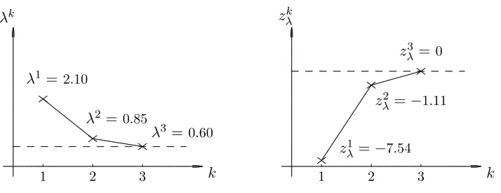
5.2.2 Dinkelbach’s Algorithm . . . 121
5.3 Sup-T Equations with a General Nonlinear Objective Function . . . 127
5.4 Sup-T Equations with a Max-Separable Objective Function . . . 130
5.4.1 Max-Separable Functions with Monotone Components . . . 131
5.4.2 Max-Separable Functions with Unimodal Components . . . 137
5.5 Bibliographical Notes . . . 141
6 Conclusions and Further Research . . . 144
6.1 Concluding Remarks . . . 144
6.2 Future Research . . . 146
6.2.1 Approximate Solutions . . . 147
6.2.2 Maximal Consistent Subsystems . . . 148
6.3 Bibliographical Notes . . . 149
LIST OF TABLES
LIST OF FIGURES
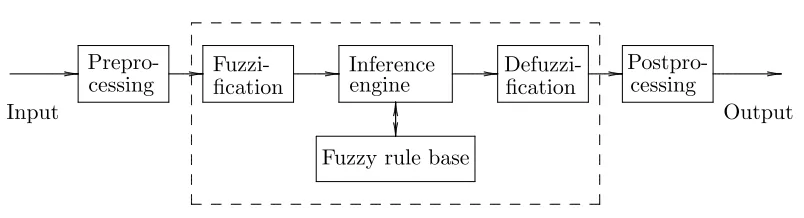
Figure 1.1 A block diagram of a fuzzy rule-based system . . . 5
Figure 2.1 The relationship between generalized logical operators . . . 19
Figure 2.2 The relationship between pairwise adjoint operators . . . 23
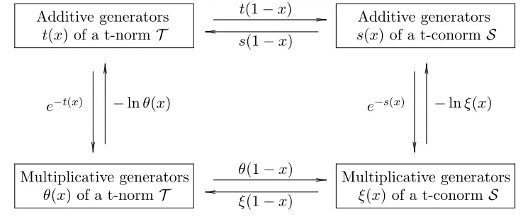
Figure 2.3 The relationship between t-norms and t-conorms and their residual operators 29 Figure 2.4 The relationship between additive and multiplicative generators . . . 40
Figure 2.5 Continuous t-norms with typical representatives of each class. . . 44
Figure 2.6 The relationship between (T,S,N) and (IT,N,JS,N,N) . . . 48
Figure 2.7 Illustrations of functionsT1(0.6, x) and T2(0.6, x) . . . 51
Figure 2.8 Illustrations of functionsS1(0.4, x) and S2(0.4, x) . . . 52
Figure 5.1 An illustration of Dinkelbach’s algorithm for Example 5.2.6 . . . 124
Chapter 1
Introduction
The aim of this dissertation is to advance our theoretical understanding of fuzzy rela-tional equations which are typically defined on the unit interval of real numbers equipped with some generalized logical operations. We provide a unified framework to characterize fuzzy relational equations of various types as well as the associated optimization problems.
1.1
Motivation
The study of fuzzy relational equations was initiated by Sanchez [399, 400, 401] in the 1970s in his pioneering work on the applications of fuzzy relations in approximate reasoning and decision making, while the notion of fuzzy relations was coined by Zadeh in his seminal paper [508] on fuzzy sets in 1965. As of today, fuzzy relational equations have played an important role as a uniform platform in a wide range of applications of fuzzy logic, particularly, in fuzzy control and knowledge engineering. The study of fuzzy relational equations is without doubt one of the most appealing subjects in the theory of fuzzy logic, from both of the mathematical and systems modeling viewpoints.
means of fuzzy relations, which form a knowledge base.
Among various types of fuzzy relational equations, finite systems of fuzzy relational equations with sup-T composition are the most fundamental and have been extensively investigated. Such a system, in most situations, can be formulated as
sup j∈N
T(aij, xj) =bi, for everyi∈M, (1.1) whereM ={1,2,· · · , m} and N ={1,2,· · · , n} are two index sets, andaij,xj, bi are real numbers in the unit interval for everyi∈M andj∈N. The compositional rule of inference applied in this case is known as the sup-T composition, more accurately, max-T composition for finite systems, where the supremum operation is interpreted as logical “OR” and the
binary operator T : [0,1]2 → [0,1] is a given triangular norm and interpreted as logical “AND”. A triangular norm, t-norm for short, is a binary operator T on the unit interval
which is commutative, associative, nondecreasing, and satisfies the boundary condition
T(1, x) = x for every x ∈[0,1]. The most frequently used t-norm in applications of fuzzy relational equations is the minimum operatorTM, i.e., TM(x, y) = min(x, y). Another two important triangular norms are theproductoperatorTP =x·y and the Lukasiewicz t-norm
TL= max(x+y−1,0).
A system of fuzzy relational equations with sup-T composition is also referred to as a system of sup-T equations for short. Usually, the t-norm T is required to be continuous, i.e., continuous as a function of two arguments. The minimum operator TM, product op-erator TP, and Lukasiewicz t-norm TL are all continuous. Actually, as will be introduced in Chapter 2, they are the most important prototypes of continuous t-norms. The study of sup-T equations with T being a continuous t-norm can be reduced, in some sense, to the study of sup-TM equations, sup-TP equations, and sup-TL equations, respectively. Be-sides, approaches to handling sup-T equations can be naturally extended to fuzzy relational equations with a general composite operation, for instance, sup-Cequations withC being a continuous conjunctor, as long as they preserve analogous structures.
DenoteA = (aij)m×n∈ [0,1]m×n, x= (xj)n×1 ∈[0,1]n and b= (bi)m×1 ∈ [0,1]m. A
finite system of sup-T equations can be represented in its matrix form as
A◦x=b, (1.2)
for a given coefficient matrixA∈[0,1]m×n and a right-hand side vectorb∈[0,1]m, i.e., to identify its solution set
S(A,b) ={x∈[0,1]n |A◦x=b}. (1.3) It is well-known in the literature that for a finite system of sup-T equationsA◦x=b
withT being a continuous t-norm, its solution set, when it is nonempty, can be characterized by one unique maximum solution and a finite number of minimal solutions, i.e.,
S(A,b) = [
ˇ
x∈Sˇ(A,b)
x∈[0,1]n |xˇ ≤x≤xˆ , (1.4) where ˇS(A,b) is the set of all minimal solutions ofA◦x=band ˆxis the maximum solution. The maximum solution can be constructed in polynomial time, while the determination of all minimal solutions is a difficult problem. Although various algorithms have been proposed during the last three decades for detecting all minimal solutions, this problem has not yet been fully resolved. Most recently, it was pointed out by Elbassioni [134] that the detection of all minimal solutions is related to the dualization problem of a monotone Boolean function, of which the exact time complexity is an unresolved problem. The best known result is attributed to Fredman and Khachiyan [143]. Besides, the influence of different t-norms on the structure of solution sets has not been fully explored.
Since solutions to a system of fuzzy relational equations may not be unique in gen-eral, solutions with some particular features are usually desired, for instance, Sanchez [401] suggested that the study of fuzzy relational equations can be extended to the study of the degree of fuzziness of the solutions. This immediately leads to the problem of optimizing an objective function (or multiple objective functions) subject to a system of fuzzy relational equations. For the case of sup-T equations, the associated optimization problem may be formulated as
min z=f(x) s.t.
A◦x=b,
x∈[0,1]n,
(1.5)
optimization problem is NP-hard even if the objective function is linear. The study of this type of optimization problems has just begun.
It has been widely recognized that there are many cross connections between mathe-matical logic and integer programming, although these two subjects are usually covered in separate texts. Fuzzy logic, as a generalization of classical Boolean logic and the mathemat-ical foundation for approximate reasoning, has been extensively studied since its inception. However, there is little work on discussing the connections between fuzzy logic and integer programming. Since fuzzy relational equations serve as a basic modeling tool for the ap-plications of fuzzy logic, the study of fuzzy relational equations as well as the associated optimization problems, from a mathematical programming perspective, would certainly ad-vance the development of fuzzy logic and provide a quantitative approach to fuzzy logical inference. Although some work has been done along this direction, a systematic treatment is absent from the known literature.
It should be noted that fuzzy relational equations, although originated from the ap-plications of fuzzy logic, can be viewed as equations over a specific residuated lattice, and hence, can be studied in a fairly independent manner not being linked to any particular application of fuzzy logic. Resolution of fuzzy relational equations from this perspective has been comprehensively discussed by De Baets [80] and Li and Fang [270].
1.2
Connection to Approximate Reasoning
consequents may involve linguistic terms. By suitable rules of inference and composition, the inference engine evaluates the input for each rule, and then determines what piece of knowledge to use next.
... ... ... ... ... ... ... ... ... ... ... ... ... ...... ... ...... ... ... .... ... ... . ...
Prepro-cessing Fuzzi-fication
Defuzzi-fication Inference engine Postpro-cessing
Fuzzy rule base Fuzzy rule-based system
Input Output ... ... ... ... ... ... ... ... ... ... ... ... ... ... ... ... ... ... ... ... ... ... ... ... ... ... ... ... ... ... ... ... ... ... ... ... ... ... ... ... ... ... ... ... . ... ... . ... ... . ... ... . ... ... . ... ... . ... ... . ... ... . ... ... . ... ... ... . ... ... . ... ... . ... ... . ... ... . ... ... . ... ... . ... ... . ... ... . ...
Figure 1.1: A block diagram of a fuzzy rule-based system
Modeling a fuzzy rule-based system is, in its very essence, to identify an appropri-ate collection of fuzzy if-then rules and incorporappropri-ate them into a specific inference scheme. According to the inference schemes applied, the vast majority of existing fuzzy rule-based systems can be roughly categorized into Mamdani-Assilian models and Takagi-Sugeno mod-els, which differ fundamentally in the formulation of if-then rules, and thus differ in the composition and defuzzification procedures accordingly. A Mamdani-Assilian model, also referred to as a linguistic fuzzy model, uses if-then rules with both fuzzy antecedents and consequents, and is essentially a qualitative expression of the concerned system. The trans-formation of the fuzzy if-then rules into a system of fuzzy relational equations has been a core idea in the procedure for developing a Mamdani-Assilian model. A Takagi-Sugeno model uses if-then rules with fuzzy antecedents and functional consequents, and is essen-tially an integrated qualitative and quantitative expression of the concerned system. For the fuzzy if-then rules of a Takagi-Sugeno model, the functional consequents are often avail-able objective knowledge of the system while the fuzzy antecedents can be determined by minimizing the quadratic error in approximation.
A typical fuzzy if-then rule for a Mamdani-Assilian model is of the form: “ifx isP, theny is Q,”
the antecedentP and consequentQare imprecise predicates, usually expressed by linguistic terms, on X and Y, respectively. For instance, in an inventory control system, a fuzzy if-then rule could be
“if inventory is high, then production should be slowed.”
The knowledge base of such a fuzzy rule-based system is represented by a finite list of fuzzy if-then rules:
ifx isAi, theny is Bi, i= 1,2, . . . , m,
and realized by a finite family{(Ai, Bi)}1≤i≤m of fuzzy input-output data pairs in an input space X and an output space Y. These fuzzy if-then rules describe a fuzzy mapping ΦR from the input space X to the output spaceY, and the data are supposed to characterize the fuzzy mapping ΦRsufficiently well. Hence, leaving aside the appropriateness of the rule list, a major problem in building up such a knowledge base for a fuzzy rule-based system is to construct the mapping ΦR from the data such that
ΦR(Ai) =Bi, i= 1,2, . . . , m. (1.6)
Following the idea of the compositional rule of inference introduced by Zadeh [509], the fuzzy mapping ΦR can be represented by a fuzzy relationR which connects fuzzy inputA and fuzzy outputB via
B =A◦R, (1.7)
with “◦” standing for a specific sup-T composite operation. Consequently, the construction of the fuzzy mapping ΦR to realize the rule list is equivalent to finding a solution to the corresponding system of sup-T equations:
Ai◦R =Bi, i= 1,2, . . . , m, (1.8)
where each equationAi◦R=Bi represents the generalized inference rule of modus ponens: ifx is Ai, theny is Bi
x is Ai
Note that, as illustrated by Dubois and Prade [130], fuzzy if-then rules may be formulated into different forms. The representation of fuzzy if-then rules is usually not unique, which results in fuzzy relational equations with various composite operations in the realization of fuzzy if-then rules. Moreover, as argued by Trillas et al. [437], the interpretation of fuzzy if-then rules depends on application context, and hence, there is no universal representation method.
The design of the fuzzy rule base, as well as its realization, is a key issue for the good performance of a fuzzy rule-based system. When the input/output dimensions are large, the design of an appropriate fuzzy rule base is a complicated task and could be time consuming.
1.3
Connection to Max-Plus Algebra
Since the late 1950s, it has been discovered independently by a number of researchers that a wide class of problems in operations research and computer science can be expressed in an attractive formulation using the framework of semirings, among which the max-plus algebra is of remarkable significance. A semiring consists of a basic set endowed with two associative binary operations which, with some additional requirements, resemble the roles of addition and multiplication in classical linear algebra, respectively. The unit interval [0,1] endowed with the maximum operation as addition and a t-norm as multiplication is a specific semiring, and hence, also referred to as the fuzzy algebra in the context of fuzzy logic. The max-plus algebra is the set of extended real numbers R∪ {−∞} endowed with the maximum operation as addition and the conventional addition as multiplication. A significant effort has been developed to build up a theory of max-plus algebra analogous to that of classical linear algebra, i.e., to study systems of linear equations, eigenvalues, rank, etc. The comprehensive guides on the algebraic properties of the max-plus algebra and its applications can be found in Cuninghame-Green [65, 67], Zimmermann [527], Baccelli et al. [11], Gaubert [145], De Schutter [88], and Gondran and Minoux [169].
Suppose that a factory manufactures productsP1, P2, . . . , Pm, each of which is made out of some ofncomponents. There arenmachines available in the factory while each machine can prepare only one fixed component to be used in several products. It is known that machineMj requiresaij time units to prepare the component independently for productPi with the convention that aij =−∞ if there is no need of the component made on machine
Mj to produce Pi. Denote by x1, x2, . . . , xn the starting times of the work on machines
M1, M2, . . . , Mn, respectively. The components necessary for product Pi will be ready at time maxj∈N(aij+xj) for everyi∈M whereM ={1,2, . . . , m}and N ={1,2, . . . , n}. On the other hand, by technological reasons, the further processing of the components can start only at some specific momentsb1, b2, . . . , bm. In order to minimize the processing inventory during the preparation stage, the problem is to find the solutions to the following system of max-plus equations
max
j∈N(aij+xj) =bi, for every i∈M, (1.9) which can be represented as A◦x = b in matrix form. It is clear that by starting early enough, all the components can be prepared before any given target times. Consequently, a way of finishing the preparation of all the components exactly on time can be obtained by artificially imposing delays. This would mean, however, the machines are not utilized in an optimal manner. Hence, obtaining the exact solutions to the system of max-plus equations
A◦x =bis of importance for optimal production planning. However, in case the system
A◦x=bhas no solution, an approximate solution of particular properties would be desired, which leads to a global optimization problem:
min ρ(A◦x−b) s.t.
x∈[−∞,+∞)n,
(1.10)
whereρ: [−∞,+∞)n→[0,+∞] is a specific index function of performance.
From the perspective of semirings, see e.g., Hebisch and Weinert [203] and Golan [163], both of the fuzzy algebra and the max-plus algebra are specific commutative idempotent semirings. Consequently, sup-T equations and max-plus equations are linear equations over their respective underlying semiring structures, and hence, have many common features, e.g., solvability criteria and structures of solution sets. Methods developed for solving sup-T
in Chapter 6, obtaining approximate solutions to a system of sup-T equations, as well as max-plus equations, is in general a hard problem except for the cases that use the Chebyshev distance as the performance index. The problem of finding Chebyshev approximate solutions for max-plus equations has been discussed by Cuninghame-Green [65, 67] and Cechl´arov´a and Cuninghame-Green [49].
Another related example is the so-called max-separable optimization problem proposed by Zimmermann [520, 521] when solving some facility location problems. For instance, sup-pose that an emergency service system, consisting n service centers S1, S2, . . . , Sn, should be built to serve m customers located at Y1, Y2, . . . , Ym. These service centers should be placed onn given segments A1B1, A2B2, . . . , AnBn, and as close as possible to the recom-mended locations C1, C2, . . . , Cn, respectively. Assume that the distances |AjBj|, |AjCj|,
|YiAj| and |YiBj| are all known and denoted by dj, cj, aij and bij, respectively, for every
i∈M and j ∈N where M ={1,2, . . . , m} and N ={1,2, . . . , n}. If we require that each customer can be served always by at least one center within a certain distance, then we obtain a system of inequalities
min
j∈Nmin(aij+xj, bij +dj −xj)≤ri, for everyi∈M, (1.11) wherexj =|AjSj|for everyj∈N andriis the specified distance threshold for everyi∈M. Consequently, we have to solve the following optimization problem:
min max
j∈N |xj−cj|
s.t.
min
j∈Nmin(aij+xj, bij+dj −xj)≤ri, for everyi∈M, 0≤xj ≤dj, for everyj∈N.
(1.12)
This problem, as indicated by Hudec [209], is NP-hard in general. However, under some additional assumptions, Tharwat and Zimmermann [432] showed that this problem can be solved efficiently by modifying the method proposed in Zimmermann [523]. Note that the method presented in Theorems 5.4.1 and 5.4.5 coincides, in its very essence, with that presented in Zimmermann [523] and Tharwat and Zimmermann [432]. See Li and Fang [272] for details.
1.4
Contributions
This dissertation studies finite systems of fuzzy relational equations over the unit in-terval from the perspective of mathematical programming. The major contributions of this dissertation are:
• It shows that a system of fuzzy relational equations can be described by an interval-valued matrix, referred to as its characteristic matrix, and hence, can be expressed in terms of 0-1 mixed integer programming formulations. This provides a new and alternative characterization of a system of fuzzy relational equations. Moreover, the relation between minimal solutions to a system of sup-T equations and irredundant coverings of its characteristic matrix is fully characterized according to the well-known representation theorem of continuous triangular norms. It shows that a minimal solution to a system of sup-T equations corresponds to an irredundant covering of its simplified characteristic matrix and vice versa, as long as the involved continuous triangular normT is Archimedean. WhenT is non-Archimedean, it corresponds to a constrained irredundant covering of the augmented characteristic matrix but not vice versa. Part of these results have been published in Li and Fang [268] and Liet al.[275]. Note that some results in Section 4.2.1 and Section 4.3.1 are generalizations of the results in Peeva [361, 366], Markovskii [296, 297], and Peeva and Kyosev [369, 370], where only the sup-TP equations or sup-TM equations involved. The results on sup-T
equations with T being a continuous Archimedean t-norm observed by Stamou and Tzafestas [420] are generalized in Section 4.2.1 as well.
• It shows that the problem of minimizing an objective function subject to a system of fuzzy relational equations can be reduced in general to a 0-1 mixed integer pro-gramming problem in polynomial time. In particular, if the objective function is linear, or more generally, separable and monotone in each argument, then it can be further reduced to a set covering problem. Besides, when the objective function is linear fractional, it can be reduced to a 0-1 linear fractional problem and then solved via parameterization methods. Part of these results have been published in Li and Fang [268, 271] and Li et al. [275].
monotone or unimodal components subject to a system of fuzzy relational equations can be solved efficiently. Furthermore, the set of optimal solutions of such a prob-lem can be well characterized. Part of these results have been published in Li and Fang [272]. Note that some results presented in Section 5.4 coincide, in the very essence, with those in Zimmermann [523] and Tharwat and Zimmermann [432].
1.5
Organization
The rest of this dissertation is organized as follows. Chapter 2 introduces the general-ized logical operators and their properties with an emphasis on continuous triangular norms. We also investigate elementary fuzzy relational equations induced by generalized logical op-erators. Chapter 3 classifies fuzzy relational equations into different categories according to the composite operations used, and discusses their solvability criteria and structures of solution sets. Chapter 4 focuses on sup-T equations and reveals the underlying connections between fuzzy relational equations and integer programming formulations. Chapter 5 illus-trates that how the sup-T equation constrained optimization problems can be reformulated into 0-1 mixed integer programming problems. In particular, we show that the reformu-lation can be further simplified when the objective function is linear or linear fractional. The max-separable optimization problem is discussed as well. Chapter 6 presents some concluding remarks and interesting topics for further research.
The bibliographical notes at the end of each chapter are intended to provide the reader with references to the works in which important contributions were first made, with infor-mation on alternative treatments of topics covered in the text, and with suggestions for further reading.
The reference list at the end of the dissertation comprises mainly the works cited in the text and notes, and covers virtually most relevant books and significant papers on fuzzy relational equations published prior to 2009.
1.6
Bibliographical Notes
precisely defined criteria of membership. Abandoning the principle of excluded middle, Zadeh introduced in 1965 in his seminal paper [508] the notion of fuzzy sets to represent such classes of objects. Although the term fuzzy often carries a pejorative connotation, the mathematics of fuzzy set theory and fuzzy logic is precise. It provides formalized tools for dealing with imprecise information and modeling complex systems in a human style of reasoning. The mathematical foundation of fuzzy logic has been discussed by Gottwald [174, 178], H´ajek [193], Nov´ak et al. [327], Gerla [153], and Bˇelohl´avek [17]. General discussion on fuzzy logic can be found in Wang et al. [458], Zadeh [510, 511, 512], and references therein.
Zadeh [509] introduced the notion of principle of incompatibility by which it means that “as the complexity of a system increases, our ability to make precise and yet signif-icant statements about its behavior diminishes until a threshold is reached beyond which precision and significance (or relevance) become almost mutually exclusive characteristics.” By this principle, Zadeh [509] argued that the conventional quantitative techniques of system analysis are intrinsically unsuited for dealing with humanistic systems or systems of com-parable complexity. Instead, Zadeh [509] outlined an alternative approach, now commonly known as fuzzy systems modeling, which is based on the premise that the key elements in human thinking are linguistic fuzzy values rather than crisp numbers. This proposal led to the development of a new class of systems based on fuzzy logic.
Mamdani and Assilian [295] implemented a linguistic fuzzy model for the first time in the form of fuzzy controllers. Linguistic fuzzy models were also investigated by King and Mamdani [237], Mamdani [294], Tong [434, 435], Mizumoto et al. [306, 307, 308], Procyk and Mamdani [382], Larsen [259], Umbers and King [439], Czoga la and Pedrycz [70], Mizu-moto and Zimmermann [309], Pedrycz [346], Buckley [29, 30], Sugeno and Yasukawa [425], Kosko [256], Ying [501], Ying and Chen [506], Castro and Delgado [43], Zeng and Singh [514], Ding et al [90], and many other researchers.
Some theoretical issues on the connections between fuzzy if-then rules of linguistic fuzzy models and fuzzy relational equations were discussed by Nov´ak and Lehmke [326], Perfilieva [372], Perfiliva and Nov´ak [375], and Gottwald [180].
available objective knowledge can hardly be incorporated into the linguistic fuzzy models if it cannot be properly represented in linguistic terms.
Takagi and Sugeno [427, 428] and Sugeno and Kang [423, 424] proposed a new type of fuzzy rule-based systems, now commonly referred to as Sugeno models or Takagi-Sugeno-Kang models, with a hybrid qualitative/quantative formulation of if-then rules. The fundamental conception of Takagi-Sugeno models is to decompose a complex system in a fuzzy manner into simpler subsystems. See also Buckley [31], Ying [502, 503], Ying et al. [507], and references therein.
General discussion on fuzzy rule-based systems can be found in Pedrycz [349], Kan-del [222], Yager and Filev [495], Geyer-Schulz [154], Ruan and Kerre [392], Ying [505], Piegat [379], and Pedrycz and Gomide [359].
The study of relational equations can be traced back to the work of L¨owenheim [284]. Equations defined on Boolean lattices have been exclusively investigated by Rudeanu [393, 394, 395, 396] in the 1970s. A comprehensive overview of equations on Boolean lattices can be found in Rudeanu [397].
Shortly after Zadeh [508] proposed the concepts of fuzzy sets and fuzzy relations in 1965, Goguen [162] indicated that fuzzy sets, as well as fuzzy relations, can be considered in a general mathematical framework of lattice. So far, two approaches of mathematical treatment have been developed when concerning the solvability of fuzzy relational equations. The first approach follows the idea of Goguen [162] and concerns the restriction on the structure of the lattice that results in fuzzy relational equations on various lattices. The second approach is developed for fuzzy relational equations on a given lattice with different types of composite operations.
The pioneering work on the application of max-plus algebra includes Shimbel [416], Kleene [240], Roy [391], Cuninghame-Green [62, 63], Giffler [159, 160], Peteanu [378], Carr´e [42], Minieka and Shier [301], Rinnooy Kan [387], Wongseelashote [479], Zimmer-mann [519], and Rote [390]. In the context of max-plus algebra, the symbols⊕ and ⊗are commonly used to denote the maximum operation and the conventional addition, respec-tively.
As of today, fuzzy relational equations have been widely applied in artificial intelli-gence, information processing, patten analysis and classification, system control, decision making and management, etc. See, e.g., Sugeno [422], Pedrycz [349, 354], Kerre and Nachte-gael [228], Szczepaniak et al. [426], Mordeson and Malik [311], Peeva and Kyosev [369], Kahraman [221], and Kerre [227].
In the context of fuzzy logic, fuzzy relational equations were first formulated and in-vestigated by Sanchez [399, 400, 401] in 1970s with an emphasis on their applications in medical diagnosis. Zadeh and Desoer [513] showed that the study of relations is equivalent to the general study of systems since a system can be viewed as relations between an input space and an output space, which can be possibly modeled into a system of fuzzy relations. Investigating the behavior of such systems requires a powerful theoretical tool to deal with fuzzy relations, typically methods for formulating and solving systems of fuzzy relational equations.
The solvability criteria of sup-TM equations were established by Sanchez [400] and then extended to sup-T equations by Pedrycz [343, 347] and Miyakoshi and Shimbo [303]. The structure of the solution set of sup-TM equations was characterized by Sanchez [401] and generalized to sup-T equations by Di Nola et al. [99, 107]. Properties of sup-T equations were also discussed by Bour and Lamotte [24], Di Nola et al. [103], Gottwald [174, 177], Klir and Yuan [248], and Li and Fang [268].
problem is closely related to the dualization problem of a monotone Boolean function, of which the exact time complexity remains an open problem. The theoretically best known algorithm for solving the dualization problem of a monotone Boolean function is due to Fredman and Khachiyan [143], which runs in incremental quasi-polynomial time. See also Khachiyanet at.[229, 230], Eiteret at.[133], and references therein for detailed discussion. The theory and applications of fuzzy relational equations developed up to 1989 were well documented by Di Nolaet al. in the first monograph [116] on this issue. Some overviews and surveys can also be found in Di Nola et al.[107, 106], Perfilieva [371], Gottwald [174, 177, 179], Klir and Yuan [248], Pedrycz [354, 357], and Peeva and Kyosev [369].
The problem of minimizing a linear objective function subject to a system of sup-TM equations was first investigated by Fang and Li [136] and later by Wu et al.[487] and Wu and Guu [485]. It was shown that such an optimization problem can be decomposed into two subproblems, one of which can be solved analytically while the other can be polynomi-ally reduced to a 0-1 integer programming problem. This observation holds true for sup-T
equations as well as equations with some other composite operations. A thorough investi-gation of sup-T equation constrained linear optimization problems is provided by Li and Fang [268]. See Section 5.5 for more details.
Chapter 2
Generalized Logical Operators
Fuzzy logic is usually considered as an extension of the classical Boolean logic. However, the generalization of classical logical operators is not unique in fuzzy logic. It is implicitly accepted from the very beginning that, for each particular problem, there associates some generalized logical operators that are better suited than others. Consequently, the study of generalized logical operators becomes one of the most active research topics of fuzzy logic. This chapter presents an overview of various types of generalized logical operators and their roles in construction and resolution of fuzzy relational equations. The material presented is essentially from Klementet al. [243] and Alsina et al. [5].
2.1
Generalized Logical Operators
Definition 2.1.1. A conjunctor C : [0,1]2 → [0,1] is a binary operator on [0,1] such that
C(0,1) =C(1,0) = 0, C(1,1) = 1, and
C(x1, y1)≤ C(x2, y2), whenever x1 ≤x2 and y1 ≤y2. (2.1)
A border conjunctor is a conjunctor that satisfies the neutrality principle, i.e., C(1, y) =y
for everyy ∈[0,1].
Definition 2.1.2. A disjunctor D : [0,1]2 → [0,1] is a binary operator on [0,1] such that
D(0,1) =D(1,0) = 1, D(0,0) = 0, and
A border disjunctor is a disjunctor that satisfies the neutrality principle, i.e., D(0, y) =y
for everyy ∈[0,1].
Note that for any conjunctorC, it holds that
C(x,0) =C(0, y) = 0, for everyx, y∈[0,1], (2.3)
while for any disjunctor D, it holds that
D(x,1) =D(1, y) = 1, for everyx, y∈[0,1]. (2.4) In other words, 0 is azero elementof a conjunctor while 1 is azero elementof a disjunctor. Definition 2.1.3. A triangular seminorm C (t-seminorm for short) is a conjunctor that satisfies the boundary condition C(x,1) = C(1, x) = x for every x ∈ [0,1]. A triangular semiconormD(t-semiconorm for short) is a disjunctor that satisfies the boundary condition
D(x,0) =D(0, x) =x for everyx∈[0,1].
Definition 2.1.4. An implicatorI : [0,1]2 →[0,1] is a binary operator on [0,1] such that
I(0,0) =I(1,1) = 1, I(1,0) = 0, and
I(x1, y)≥ I(x2, y), whenever x1 ≤x2; (2.5)
I(x, y1)≤ I(x, y2), whenever y1 ≤y2. (2.6) A border implicator is an implicator that satisfies the neutrality principle, i.e., I(1, y) =y
for everyy ∈[0,1].
Definition 2.1.5. A coimplicatorJ : [0,1]2 →[0,1]is a binary operator on [0,1]such that
J(0,0) =J(1,1) = 0, J(0,1) = 1, and
J(x1, y)≥ J(x2, y), whenever x1 ≤x2; (2.7)
J(x, y1)≤ J(x, y2), whenever y1 ≤y2. (2.8)
A border coimplicator is a coimplicator that satisfies the neutrality principle, i.e., J(0, y) =
y for every y∈[0,1].
Note that for any implicatorI, it holds that
while for any coimplicatorJ, it holds that
J(x,0) =J(1, y) = 0, for everyx, y∈[0,1]. (2.10) These boundary properties are also referred to as the absorption principles.
Definition 2.1.6. A negatorN : [0,1]→[0,1]is a decreasing unary operator on [0,1]such thatN(0) = 1and N(1) = 0. A negatorN is called strict if it is bijective. A strict negator
N is called strong if it is involutive, i.e.,N(N(x)) =x for everyx∈[0,1].
A negatorN defined on the unit interval is strict if and only if it is strictly decreasing and continuous. Moreover, ifN is a strong negator, thenN−1(x) =N(x) for everyx∈[0,1],
where N−1 is the inverse operator of N. A full characterization of strong negators was
provided by Trillas [436].
Theorem 2.1.7. The unary operator N : [0,1] → [0,1] is a strong negator if and only if there is a monotone bijection ψ: [0,1]→[0,1] such that, for every x∈[0,1],
N(x) =ψ−1(1−ψ(x)). (2.11) In particular, the negatorNs withNs(x) = 1−x is called the standard negator or the Lukasiewicz negator, which is also the most important and the most widely used one in practice. As a consequence of Theorem 2.1.7, each strong negatorN is a ψ-transformation of the standard negatorNs, i.e.,
N(x) =ψ−1(Ns(ψ(x)), (2.12) whereψ: [0,1]→[0,1] is a monotone bijection on [0,1]. Besides, any implicatorI induces a negatorNI(x) =I(x,0), and any coimplicatorJ also induces a negator NJ(x) =J(x,1). Conversely, an implicator can be defined by a conjunctorC and a negator N via
IC,N(x, y) =N(C(x,N(y))), (2.13) while a coimplicator can be defined by a disjunctorD and a negatorN via
JD,N(x, y) =N(D(x,N(y))). (2.14) Similarly, a conjunctor can be defined by an implicatorI and a negatorN via
while a disjunctor can be defined by a coimplicatorJ and a negatorN via
DJ,N(x, y) =N(J(x,N(y))). (2.16) Furthermore, with a strong negatorN, a conjunctor Ccan be induced by a disjunctor
D and vice versa, i.e.,
C(x, y) =N(D(N(x),N(y))), (2.17)
D(x, y) =N(C(N(x),N(y))); (2.18) and an implicator I can be induced by a coimplicator J and vice versa, i.e.,
I(x, y) =N(J(N(x),N(y))), (2.19)
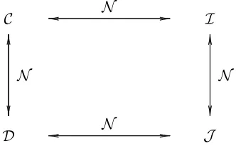
J(x, y) =N(I(N(x),N(y))). (2.20) In this sense, a triple (C,D,N), as well as (I,J,N), forms a De Morgan triple where the conjunctor C and the disjunctor D are dual to each other with respect to the strong negator N. Furthermore, a pair of De Morgan triples (C,D,N) and (I,J,N) are said to be isomorphic if I =IC,N or equivalently, C =CI,N. For any De Morgan triple (C,D,N), its isomorphic De Morgan triple (I,J,N) is uniquely determined and vice versa. It is clear that for a pair of isomorphic De Morgan triples (C,D,N) and (I,J,N), the conjunctorC
is a border conjunctor if and only if the implicatorI is a border implicator, or equivalently, if and only if the disjunctorDand the coimplicatorJ are a border disjunctor and a border coimplicator, respectively. The relations between these generalized logical operators are illustrated in Figure 2.1.
C I D J ... . . . . . . . . . . . . . . . ... ... N ... . . . . . . . . . . . . . . . ... ... N ... ... ... ... ... ... ... ... ... ... ... ... ... ... ... . ... ... ... ... ... ... ... ... ... ... ... ... ... ... ... ... ... ... ... ... ... ... ... ... ... ... ... ... N N ... ... ... ... ... ... ... ... ... ... ... ... ... ... ... . ... ... ... ... ... ... ... ... ... ... ... ... ... ... ... ... ... ... ... ... ... ... ... ... ... ... ... ... ...
Figure 2.1: The relationship between generalized logical operators
Definition 2.1.8. The residual implicator IC and its accompanied residual operator JC with respect to a border conjunctor C are defined, respectively, as
IC(x, y) = sup{z∈[0,1] | C(x, z)≤y}, (2.21)
JC(x, y) = inf{z∈[0,1]| C(x, z)≥y}. (2.22)
It can be verified that the residual implicatorICis indeed a border implicator while the operatorJChas no particular logical interpretation. Note that the residual operatorsIC and
JC can actually be defined for any conjunctorC. However, IC may fail to be an implicator whenCis not a border conjunctor. Moreover, the definitions of these two residual operators are not unique when the conjunctorC is not commutative. The left residual operators with respect to a conjunctorC can be defined accordingly.
Dually, the residual operatorsID andJDcan be defined with respect to a given border disjunctorD.
Definition 2.1.9. The residual coimplicator JD and its accompanied residual operatorID with respect to a border disjunctor D are defined, respectively, as
JD(x, y) = inf{z∈[0,1] | D(x, z)≥y}, (2.23)
ID(x, y) = sup{z∈[0,1] | D(x, z)≤y}. (2.24)
It can be verified that the residual coimplicator JD is a border coimplicator while the operator ID has no particular logical interpretation. With the infix notations, IC(x, y) and JC(x, y) are denoted by xϕcy and xσcy, respectively, while ID(x, y) and JD(x, y) are denoted by xβdy andxωdy, respectively.
Analogously, residual operators can be defined with respect to border implicators and border coimplicators, respectively.
Definition 2.1.10. The residual conjunctor CI and its accompanied residual operator DI with respect to a border implicator I are defined, respectively, as
CI(x, y) = inf{z∈[0,1] | I(x, z)≥y}, (2.25)
Definition 2.1.11. The residual disjunctor DJ and its accompanied residual operator CJ with respect to a border coimplicator J are defined, respectively, as
DJ(x, y) = sup{z∈[0,1]| J(x, z)≤y}, (2.27)
CJ(x, y) = inf{z∈[0,1]| J(x, z)≥y}. (2.28) The residual operator CI is always a border conjunctor while the residual operator
DJ is always a border disjunctor. The operators DI and CJ have no particular logical interpretation. With the infix notations, CI(x, y) and DI(x, y) are denoted by xγIy and
xδIy, respectively, whileDJ(x, y) andCJ(x, y) are denoted byxδJyandxγJy, respectively. As has been shown, the residual operators of border conjunctors and border disjunctors lead to border implicators and border coimplicators, respectively, and vice versa. Moreover, they form pairs of adjoint operators, respectively, under additional residuation conditions. Definition 2.1.12. A function f : [0,1] → [0,1] is said to be lower semicontinuous if
{x ∈ [0,1] | f(x) > α} is an open set for every α ∈ [0,1], and upper semicontinuous if
{x∈[0,1]| f(x)< α} is an open set for everyα∈[0,1].
Definition 2.1.13. A functionf : [0,1]→[0,1]is said to be left-continuous if lim x→x0−
f(x) =
f(x0)for everyx0 ∈(0,1], and right-continuous if lim x→x0+
f(x) =f(x0)for everyx0 ∈[0,1). A function f : [0,1] → [0,1] is said to be continuous if lim
x→x0
f(x) = f(x0) for every
x0 ∈[0,1].
Theorem 2.1.14. A function f : [0,1]→[0,1] is continuous if and only if it is both left-and right-continuous, or both lower left-and upper semicontinuous.
Theorem 2.1.15. An increasing functionf : [0,1]→[0,1] is lower semicontinuous if and only if it is left-continuous, and upper semicontinuous if and only if it is right continuous. Note that the left- and right-continuity mean exactly the interchangeability of the supremum operation and the infimum operation, respectively, with an increasing function. Theorem 2.1.16. Let C : [0,1]2 → [0,1] be a border conjunctor andI
C its residual impli-cator. The following statements are equivalent:
(i) The conjunctorC and the implicator IC form a pair of adjoint residual operators, i.e., for anya, b∈[0,1],
(ii) The second partial mapping of C, i.e., C(a,·), is left-continuous for every a∈[0,1]. (iii) The second partial mapping ofIC, i.e.,IC(a,·), is right-continuous for everya∈[0,1]. Theorem 2.1.17. If C : [0,1]2 → [0,1] is a border conjunctor with its second partial mapping C(a,·) being left-continuous for everya∈[0,1], then CIC =C.
Proof. It follows Theorem 2.1.16 that for any x, y∈[0,1],
CIC(x, y) = inf{z∈[0,1]| IC(x, z)≥y}
= inf{z∈[0,1]| C(x, y)≤z}
=C(x, y).
Theorem 2.1.18. Let D: [0,1]2 →[0,1] be a border disjunctor and JD its residual coim-plicator. The following statements are equivalent:
(i) The coimplicator JD and the disjunctor D form a pair of adjoint residual operators, i.e., for any a, b∈[0,1],
JD(a, x)≤b if and only if x≤ D(a, b). (2.30)
(ii) The second partial mapping ofJD, i.e.,JD(a,·), is left-continuous for everya∈[0,1]. (iii) The second partial mapping of D, i.e., D(a,·), is right-continuous for every a∈[0,1]. Theorem 2.1.19. If D : [0,1]2 → [0,1] is a border disjunctor with its second partial mapping D(a,·) being right-continuous for every a∈[0,1], then DJD =D.
Proof. It follows Theorem 2.1.18 that for any x, y∈[0,1],
DJD(x, y) = sup{z∈[0,1]| JD(x, z)≤y}
= sup{z∈[0,1]| D(x, y)≥z}
=D(x, y).
C IC
D JD
... . . . . . . . . . . . . . . . ... ... R ... . . . . . . . . . . . . . . . ... ... R ... ... ... ... ... ... ... ... ... ... ... ... ... ... ... . ... ... ... ... ... ... ... ... ... ... ... ... ... ... ... ... ... ... ... ... ... ... ... ... ... ... ... ... N N ... ... ... ... ... ... ... ... ... ... ... ... ... ... ... . ... ... ... ... ... ... ... ... ... ... ... ... ... ... ... ... ... ... ... ... ... ... ... ... ... ... ... ... ...
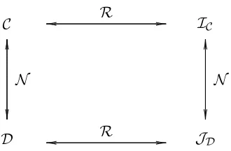
Figure 2.2: The relationship between pairwise adjoint operators
Definition 2.1.20. Let C: [0,1]2→[0,1] be a conjunctor. An elementa∈(0,1]is said to be a left zero divisor of C if there exists some b∈(0,1] such that C(a, b) = 0. Analogously, an element b ∈ (0,1] is said to be a right zero divisor of C if there exists some a ∈ (0,1] such that C(a, b) = 0. An element that is both a left and a right zero divisor is simply called a zero divisor.
The left and right zero divisors are the same when the conjunctor is commutative. A nonzero element is called regular if it is neither a left nor a right zero divisor of the conjunctor.
Definition 2.1.21. Let D: [0,1]2 →[0,1] be a disjunctor. An elementa∈[0,1)is said to be a left zero divisor of Dif there exists some b∈[0,1)such thatD(a, b) = 1. Analogously, an element b ∈[0,1) is said to be a right zero divisor of D if there exists some a ∈[0,1) such thatD(a, b) = 1. An element that is both a left and a right zero divisor is simply called a zero divisor.
Note that 1 is the “zero element” with respect to a disjunctor by Definition 2.1.2. Analogous concepts can be defined as well for implicators and coimplicators according to their respective absorption principles.
Definition 2.1.22. Let I : [0,1]2 → [0,1] be an implicator. An element a∈(0,1] is said to be a left zero divisor of I if there exists someb∈[0,1)such that I(a, b) = 1. An element
b ∈ [0,1) is said to be a right zero divisor of I if there exists some a ∈ (0,1] such that
Definition 2.1.23. Let J : [0,1]2 → [0,1] be a coimplicator. An element a ∈ [0,1) is said to be a left zero divisor of J if there exists some b∈(0,1] such that J(a, b) = 0. An element b∈(0,1] is said to be a right zero divisor of J if there exists some a∈[0,1) such thatJ(a, b) = 0.
Definition 2.1.24. Let C: [0,1]2→[0,1] be a conjunctor. (i) The conjunctor C satisfies the right cancelation law if
C(x, y) =C(x, z) implies x= 0 or y=z. (2.31)
(ii) The conjunctor C satisfies the right conditional cancelation law if
C(x, y) =C(x, z)>0 implies y=z. (2.32)
Theorem 2.1.25. Let C: [0,1]2 →[0,1] be a conjunctor.
(i) The conjunctor C satisfies the right cancelation law if and only if the second partial mapping C(x,·) is strictly increasing for every x∈(0,1], i.e.,
C(x, y)<C(x, z) whenever x >0 and y < z. (2.33)
(ii) The conjunctorCsatisfies the right conditional cancelation law if and only if the second partial mapping C(x,·) is conditionally strictly increasing for every x∈(0,1], i.e.,
C(x, y)<C(x, z) whenever C(x, y)>0 and y < z. (2.34)
Proof. If the functionC(x,·) is strictly increasing for everyx∈(0,1], then the conjunctorC
satisfies the right cancelation law. Conversely, the right cancelation law and the monotonic-ity of the conjunctor C imply that the second partial mappingC(x,·) is strictly increasing for every x ∈ (0,1]. The second assertion is an immediate consequence of the previous one.
When a conjunctor C only satisfies the right conditional cancelation law, it necessarily has right zero divisors. Analogously, the left cancelation law and the left conditional law can be defined for conjunctors. For commutative conjunctors, the terms cancelation law and conditional cancelation law may be used, respectively.
The dual versions of Definition 2.1.24 and Theorem 2.1.25 for disjunctors can be derived without any difficulty.
Definition 2.1.26. Let D: [0,1]2 →[0,1]be a disjunctor. (i) The disjunctor Dsatisfies the right cancelation law if
D(x, y) =D(x, z) implies x= 1 or y=z. (2.35)
(ii) The disjunctor Dsatisfies the right conditional cancelation law if
D(x, y) =D(x, z)>0 implies y=z. (2.36)
Theorem 2.1.27. Let D: [0,1]2 →[0,1] be a disjunctor.
(i) The disjunctor D satisfies the right cancelation law if and only if the second partial mapping D(x,·) is strictly increasing for every x∈(0,1], i.e.,
D(x, y)<D(x, z) whenever x <1 and y < z. (2.37)
(ii) The disjunctorDsatisfies the right conditional cancelation law if and only if the second partial mapping D(x,·) is conditionally strictly increasing for every x∈(0,1], i.e.,
D(x, y)<D(x, z) whenever D(x, y)<1 and y < z. (2.38)
Analogously, the right cancelation laws and the right conditional cancelation laws of implicators and coimplicators can be defined in a similar manner as those of conjunctors and disjunctors, respectively. However, the left cancelation laws and the left conditional cancelation laws of implicators and coimplicators should be defined in a dual manner. Definition 2.1.28. Let I : [0,1]2 →[0,1] be an implicator.
(i) The implicator I satisfies the left cancelation law if
(ii) The implicator I satisfies the left conditional cancelation law if
I(x, z) =I(y, z)<1 implies x=y. (2.40)
Definition 2.1.29. Let J : [0,1]2 →[0,1] be a coimplicator. (i) The coimplicator J satisfies the left cancelation law if
J(x, z) =J(y, z) implies z= 0 or x=y. (2.41)
(ii) The coimplicator J satisfies the left conditional cancelation law if
J(x, z) =J(y, z)>0 implies x=y. (2.42)
Analogous to Theorems 2.1.25 and 2.1.27, the left cancelation laws and the left con-ditional cancelation laws of implicators and coimplicators require that the implicators and coimplicators be strictly decreasing in their first arguments within proper domains, respec-tively.
For a pair of isomorphic De Morgan triples (C,D,N) and (I,J,N), the conjunctor
C satisfies the left (right) cancelation law or conditional cancelation law if and only if the implicator I satisfies the left (right) cancelation law or conditional cancelation law, or equivalently, if and only if the disjunctor D and the coimplicator J satisfy the left (right) cancelation law or conditional cancelation law, respectively. Similar results can be readily derived for the left-continuity (right-continuity) and the existence of zero divisors on the pair of isomorphic De Morgan triples (C,D,N) and (I,J,N). These relations show that there is no essential difference between these binary generalized logical operators from an algebraic point of view regardless of their specific interpretations in the general theory of logic. Consequently, it suffices to focus on some specific class of these binary generalized logical operators in the case that only algebraic properties of them are concerned, for instance, the resolution and optimization of a system of fuzzy relational equations.
2.2
Triangular Norms and Conorms
Definition 2.2.1. A triangular norm (t-norm for short) is a binary operator T : [0,1]2 →
[0,1] such that for every x, y, z∈[0,1]the following four axioms are satisfied: (T1) T(x, y) =T(y, x). (commutativity)
(T2) T(x,T(y, z)) =T(T(x, y), z). (associativity) (T3) T(x, y)≤ T(x, z), whenever y≤z. (monotonicity) (T4) T(x,1) =x. (boundary condition)
Definition 2.2.2. A triangular conorm (t-conorm or s-norm for short) is a binary operator
S : [0,1]2 →[0,1] such that for every x, y, z∈[0,1]the following four axioms are satisfied: (S1) S(x, y) =S(y, x). (commutativity)
(S2) S(x,S(y, z)) =S(S(x, y), z). (associativity) (S3) S(x, y)≤ S(x, z), whenever y ≤z. (monotonicity) (S4) S(x,0) =x. (boundary condition)
The infix notations like x∧ty and x∨ty are usually used in the literature instead of the prefix notations T(x, y) and S(x, y), respectively, whilex∧y and x∨y typically stand for theminimum operatorTM(x, y) and themaximum operatorSM(x, y), respectively.
There exist uncountably many t-norms among which four basic t-norms are remarkable from different points of view, and are defined by, respectively,
TM(x, y) = min(x, y), (minimum, G¨odel t-norm, Zadeh t-norm)
TP(x, y) =x·y, (probabilistic product, Goguen t-norm)
TL(x, y) = max(x+y−1,0), (bounded difference, Lukasiewicz t-norm)
TD(x, y) =
0, if (x, y)∈[0,1)2 min(x, y), otherwise.
(drastic product)
Their dual t-conorms with respect to the standard negatorNs are given by, respectively,
SM(x, y) = max(x, y), (maximum, G¨odel t-conorm, Zadeh t-conorm)
SP(x, y) =x+y−x·y, (probabilistic sum, Goguen t-conorm)
SL(x, y) = min(x+y,1), (bounded sum, Lukasiewicz t-conorm)
SD(x, y) =
1, if (x, y)∈(0,1]2 max(x, y), otherwise.
A t-norm T, as well as a t-conorm S, is said to be continuous if it is continuous as a real function with two arguments, i.e., for every (x0, y0)∈[0,1]2, it holds that
lim
(x,y)→(x0,y0)
T(x, y) =T(x0, y0).
Due to the monotonicity and commutativity properties of t-norms, a t-norm T is contin-uous if and only if it is contincontin-uous in each argument, and hence, if and only if its partial mapping T(a,·) is continuous for every a∈[0,1]. Consequently, a t-norm T is said to be left-continuous (right-continuous) if and only if its partial mappingT(a,·) is left-continuous (right-continuous) for everya∈[0,1]. A t-normT is continuous if and only if it is both left-and right-continuous. Moreover, Theorem 2.1.15 allows us to speak about left-continuous and right-continuous t-norms instead of lower and upper semicontinuous t-norms, respec-tively. TheminimumoperatorTM,productoperatorTP, and Lukasiewicz t-norm TLare all continuous, while thedrastic productoperatorTDis right-continuous but not left-continuous. The results for t-conorms can be derived dually.
Theorem 2.2.3. A t-norm T is left-continuous (right-continuous) if and only if its dual t-conorm S with respect to the standard negator Ns is right-continuous (left-continuous).
Themaximum operatorSM,probabilistic sum operatorSP, and Lukasiewicz t-conorm
SL are all continuous, while the drastic sum operator SD is left-continuous but not right-continuous.
As a consequence of Theorems 2.1.17 and 2.1.19, the relations between a left-continuous t-norm and its dual t-conorm and residual operators, respectively, can be illustrated as in Figure 2.3. The residual implicator IT is also called an R-implicator for short. However, only those with respect to left-continuous t-norms are of particular interest, in which case, the t-norm and its residual implicator form a pair of adjoint residual operators.
The residual operatorsIT andJT of the three most important continuous t-norms are listed in Table 2.1.
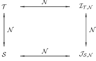
Moreover, with a De Morgan triple (T,S,N), the implicator IT,N is defined by
IT,N(x, y) =N(T(x,N(y))) =S(N(x), y), (2.43) which is also called a strong implicator, or in short form, an S-implicator. Analogously, the coimplicator JS,N is defined by
T IT
S JS
... . . . . . . . . . . . . . . . ... ... R ... . . . . . . . . . . . . . . . ... ... R ... ... ... ... ... ... ... ... ... ... ... ... ... ... ... . ... ... ... ... ... ... ... ... ... ... ... ... ... ... ... ... ... ... ... ... ... ... ... ... ... ... ... ... N N ... ... ... ... ... ... ... ... ... ... ... ... ... ... ... . ... ... ... ... ... ... ... ... ... ... ... ... ... ... ... ... ... ... ... ... ... ... ... ... ... ... ... ... ...
Figure 2.3: The relationship between t-norms and t-conorms and their residual operators
Table 2.1: Residual operators of the G¨odel, Goguen and Lukasiewicz t-norms
T IT(x, y) JT(x, y)
TM
(
1, ifx≤y y, otherwise.
(
1, ifx < y y, otherwise.
TP
(
1, ifx≤y y/x, otherwise.
1, ifx < y y/x, if 0< y ≤x
0, otherwise.
TL min(1−x+y,1)
1, ifx < y
1−x+y, if 0< y ≤x
0, otherwise.
which is also called a strong coimplicator, an S-coimplicator for short.
In addition, the induced implicator IT,N and coimplicator JS,N may reconstruct the strong negatorN, respectively, i.e.,
N(x) =IT,N(x,0) =JS,N(x,1). (2.45)
This assertion holds for t-seminorms and t-semiconorms, however, not for general conjunc-tors and disjuncconjunc-tors.
TM, theproductoperatorTP and the Lukasiewicz t-norm TL, respectively, are listed below:
ITM,Ns(x, y) = max(1−x, y), the Kleene-Dienes implicator;
ITP,Ns(x, y) = 1−x+x·y, the Reichenbach implicator;
ITL,Ns(x, y) = min(1−x+y,1), the Lukasiewicz implicator.
Note that the residual implicator ITL of the Lukasiewicz t-norm TL coincides with the
Lukasiewicz implicatorITL,Ns. Consequently, the standard negatorNscan be reconstructed
by the Lukasiewicz implicatorITL,Ns as well as the residual implicatorITL . The
coimplica-tors induced by the standard negator Ns and the corresponding t-conorms can be derived dually.
Another type of implicators, called quantum logic implicators (briefly QL-implicators) in the literature, can be defined via a t-norm T, a t-conorm S, and a strong negator N, typically a De Morgan triple (T,S,N), by
IT,S,N(x, y) =S(N(x),T(x, y)). (2.46)
In general, a QL-implicator IT,S,N is not well defined since the monotonicity in its first argument cannot be guaranteed. Some counterexamples have been constructed in Dubois et al. [124] for different classes of t-norms. A necessary condition can be obtained quickly by checking the boundary condition
IT,S,N(x,1) =S(N(x), x) = 1, for everyx∈[0,1]. (2.47)
Fodor [141] proposed some conditions under which IT,S,N becomes an implicator. In this case,IT,S,N is a border implicator and the induced negator coincides with the strong negator
N.
R-implicators, S-implicators, and QL-implicators, all of which are border implicators, are three fundamental classes of implicators used in fuzzy inference systems due to their sound logic foundation and good approximation capability. They will be further discussed in Section 2.5.
T1 ≤ T2, if the inequalityT1(x, y)≤ T2(x, y) holds for every (x, y)∈[0,1]2. Equivalently,T2
is said to be stronger than T1 if T1 ≤ T2. Moreover, the notationT1 <T2 is used whenever
T1 ≤ T2 and T1 =6 T2. It is well-known that the drastic productoperator TD is the weakest and theminimumoperatorTM is the strongest t-norm, i.e., for any t-normT, it holds that
TD ≤ T ≤ TM.
Besides, it is clear that
TD <TL<TP <TM.
Dually, the order relation reverses for t-conorms. The maximum operator SM is the weakest and the drastic sumoperator SD is the strongest t-conorm, i.e., for any t-conorm
S, it holds that
SM ≤ S ≤ SD.
Besides, it holds that
SM <SP <SL<SD.
The associativity property of t-norms allows us to uniquely extend each t-normT in a recursive manner to ann-ary operator, i.e.,
T(x1, . . . , xn) =T(T(x1, . . . , xn−1), xn)
for each n-tuple (x1, . . . , xn) ∈[0,1]n with the integer n≥3. In particular, T( n z }| {
x, . . . , x) is denoted as x(Tn) for each x ∈ [0,1] and called the nth power of x with respect to T, with the convention thatx(0)T = 1 and x(1)T =x. The n-ary extensions for the four basic t-norms are as follows:
TM(x1, x2, . . . , xn) = min(x1, x2, . . . , xn),
TP(x1, x2, . . . , xn) =x1·x2· · ·xn,
TL(x1, x2, . . . , xn) = max n
P i=1
xi−(n−1),0
,
TD(x1, x2, . . . , xn) =
Analogously, each t-conorm S can be uniquely extended to an n-ary operator, i.e.,
S(x1, . . . , xn) =S(S(x1, . . . , xn−1), xn)
for each n-tuple (x1, . . . , xn) ∈[0,1]n with the integer n≥3. In particular, S( n z }| {
x, . . . , x) is denoted asx(Sn)for eachx∈[0,1] and called thenth power ofxwith respect toS, with the convention that x(0)S = 0 and x(1)S =x. Then-ary extensions for the four basic t-conorms are as follows:
SM(x1, x2, . . . , xn) = max(x1, x2, . . . , xn),
SP(x1, x2, . . . , xn) = 1−(1−x1)(1−x2)· · ·(1−xn),
SL(x1, x2, . . . , xn) = min n
P i=1
xi,1
,
SD(x1, x2, . . . , xn) =
xi, ifxj = 0 for all j6=i, 1, otherwise.
To better understand norms and conorms, some additional algebraic properties of t-norms and t-cot-norms are necessary to be presented, most of which are well-known from the general theories of semigroups and lattices because t-norms and t-conorms can be viewed as special classes of commutative semigroups, respectively.
Definition 2.2.4. Let T : [0,1]2 →[0,1] be a t-norm.
(i) An element a∈[0,1] is called an idempotent element ofT if T(a, a) =a.
(ii) An element a∈ (0,1) is called a nilpotent element of T if there exists some positive integer n such thata(Tn)= 0.
(iii) An element a∈(0,1) is called a zero divisor of T if there exists someb∈(0,1) such thatT(a, b) = 0.
Theorem 2.2.5.
(i) An elementa∈[0,1]is an idempotent of a t-normT if and only ifT(a, x) = min(a, x) for everyx∈[a,1].
(ii) An element a ∈ [0,1] is an idempotent of a continuous t-norm T if and only if
T(a, x) = min(a, x) for everyx∈[0,1].
The product operator TP, Lukasiewicz t-norm TL, and drastic product operator TD
possess only trivial idempotent elements. The set of idempotent elements of the minimum operatorTM is [0,1]. Actually,TM is the only t-norm with this property. Furthermore, the minimum operator TM and the product operator TP have neither nilpotent elements nor zero divisors, while each a ∈ (0,1) is both a nilpotent element and a zero divisor of the Lukasiewicz t-normTL as well as the drastic product operatorTD.
Generally, each nilpotent element of a t-normT is also a zero divisor ofT but not vice versa, which means that the set of nilpotent elements is a subset of the set of zero divisors. However, the existence of zero divisors is equivalent to the existence of nilpotent elements for each t-norm, i.e., a t-norm T has zero divisors if and only if it has nilpotent elements. Moreover, if a∈(0,1) is a zero divisor of a t-normT, then each numberb ∈(0, a) is also a zero divisor of T due to the monotonicity property of T. This also holds for nilpotent elements.
Definition 2.2.6.
(i) A t-norm T is called strictly monotone if T(x, y) < T(x, z) whenever x > 0 and
y < z.
(ii) A t-norm T is called strict if it is continuous and strictly monotone.
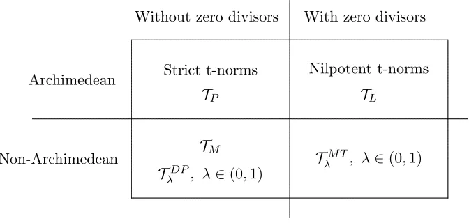
(iii) A t-norm T is called nilpotent if it is continuous and each x ∈ (0,1) is a nilpotent element of T.
(iv) A t-norm T is called Archimedean if for each (x, y) ∈ (0,1)2 there exists a positive integer n such thatx(Tn) < y.
It is evident that an Archimedean t-norm has only trivial idempotent elements. It was shown by Koles´arov´a [250] that the left-continuity of an Archimedean t-norm implies its continuity. Furthermore, Theorem 2.2.7 indicates that each strict or nilpotent t-norm is Archimedean. Moreover, it turns out that a continuous Archimedean t-norm is either strict or nilpotent. Clearly, the productoperatorTP is a strict t-norm and the Lukasiewicz t-norm TL is a nilpotent t-norm. The minimum operator TM is a continuous but not Archimedean t-norm. The drastic product operator TD is a noncontinuous Archimedean t-norm for which each x ∈ (0,1) is a nilpotent element. Besides, as a consequence of Theorem 2.1.25, each strict t-norm satisfies the cancelation law while each nilpotent t-norm satisfies the conditional cancelation law. By Theorem 2.2.5, no continuous non-Archimedean t-norm satisfies the conditional cancelation law.
Dually, these properties can be defined for t-conorms by interchanging the roles of 0 and 1.
Definition 2.2.8. Let S: [0,1]2 →[0,1]be a t-conorm.
(i) An element a∈[0,1] is called an idempotent element ofS if S(a, a) =a.
(ii) An element a∈(0,1) is called a nilpotent element of S if there exists some positive integer n such thata(Sn)= 1.
(iii) An element a∈(0,1)is called a zero divisor of S if there exists some b∈(0,1) such thatS(a, b) = 1.
Theorem 2.2.9.
(i) An element a ∈ [0,1] is an idempotent of a t-conorm S if and only if S(a, x) = max(a, x) for every x∈[a,1].
(ii) An element a ∈ [0,1] is an idempotent of a continuous t-conorm S if and only if
S(a, x) = max(a, x) for every x∈[0,1].
The numbers 0 and 1 are idempotent elements for each t-conormS, and hence, called trivial idempotent elements of S, while each idempotent element in (0,1) is called a non-trivial idempotent element of S. The probabilistic sum operatorSP, Lukasiewicz t-conorm
operator SM is the only t-conorm such that its set of idempotent elements is [0,1]. Fur-thermore, the maximum operator SM and the probabilistic sum operator SP have neither nilpotent elements nor zero divisors, while each a∈(0,1) is both a nilpotent element and a zero divisor of the Lukasiewicz t-conormSL as well as the drastic sumoperatorSD. Definition 2.2.10.
(i) A t-conorm S is called strictly monotone if S(x, y) < S(x, z) whenever x < 1 and
y < z.
(ii) A t-conorm S is called strict if it is continuous and strictly monotone.
(iii) A t-conorm S is called nilpotent if it is continuous and each x∈(0,1) is a nilpotent element of S.
(iv) A t-conormS is called Archimedean if for each(x, y)∈(0,1)2 there exists a positive
integer n such thatx(Sn) > y.
Theorem 2.2.11. A continuous t-conorm S is Archimedean if and only ifS(x, x)> x for every x∈(0,1).
It is evident that a t-conorm S is Archimedean if and only if its dual t-norm with respect to the standard negator Ns is Archimedean. A continuous Archimedean t-conorm is either strict or nilpotent. Clearly, the probabilistic sumoperator SP is a strict t-conorm and the Lukasiewicz t-conormSL is a nilpotent t-conorm. ThemaximumoperatorSM is a continuous but not Archimedean t-conorm. Thedrastic sumoperatorSD is a noncontinuous Archimedean t-conorm for which each x∈(0,1) is a nilpotent element.
2.3
Construction of Triangular Norms and Conorms
From an algebraic point of view, t-norms, as well as t-conorms, are a special class of commutative semigroups, and hence, can be constructed via various methods developed in semigroup theory.
It is straightforward that, given a t-normT, any strictly increasing bijectionψ: [0,1]→
[0,1] defines a t-norm by
Furthermore,T and Tψ are isomorphic in the sense that
ψ(Tψ(x, y)) =T(ψ(x), ψ(y)) (2.49)
for every (x, y) ∈ [0,1]2. Dually, given a t-conorm S, any strictly increasing bijection
ψ: [0,1]→[0,1] defines a t-conorm as well by
Sψ(x, y) =ψ−1(S(ψ(x), ψ(y))), (2.50)
and S and Sψ are isomorphic in the sense that
ψ(Sψ(x, y)) =S(ψ(x), ψ(y)) (2.51)
for every (x, y) ∈ [0,1]2. Clearly, T and Tψ, as well as S and Sψ, share many common structural features, e.g., continuity, Archimedean property, and the existence of idempotent and nilpotent elements as well as the existence of zero divisors. The only invariants under arbitrary strictly increasing bijections are the two extremal t-norms,TM and TD, and two extremal t-conorms, SM and SD, respectively.
A more general method to construct t-norms and t-conorms involves the pseudoinverses of monotone functions.
Definition 2.3.1. Letf : [a, b]→[c, d]be a monotone function where[a, b]and[c, d]are two closed subintervals of the extended real line [−∞,+∞]. The pseudoinverse f(−1) : [c, d]→
[a, b] is defined as
f(−1)(y) = sup{x∈[a, b]|(f(x)−y)(f(b)−f(a))<0}.
Corollary 2.3.2. Letf : [a, b]→[c, d]be a monotone function where[a, b]and[c, d]are two closed subintervals of the extended real line [−∞,+∞]. The pseudoinverse f(−1) : [c, d]→