[NORMAL] Influence of Surface Heterogeneities on the Boundary Layer Structure and Diffusion of Pollutants

ABSTRACT

Robert C. Gilliam: Influence of Surface Heterogeneities on the Boundary

Layer Structure and Diffusion of Pollutants. (Under the direction of Dr.

Sethu Raman)

Boundary layer processes are the dominating factors in the diffusion and transport of pollutants. Air pollution dispersion is known to be controlled by several boundary layer factors. Eddy diffusion, described by the amount of turbulent kinetic energy, is the main influence on how quickly a parcel of polluted air expands and boundary layer depth determines the extent of vertical mixing potential.

This thesis explores the influence that mesoscale surface related features have on the boundary layer meteorology and air pollution dispersion through a combination of numerical model simulations and observations. Mesoscale processes including sea breeze and land breeze circulations, vegetation and soil type gradient induced circulations, urban heat island and terrain modified flows are addressed in this research through the use of various numerical simulations. Surface based observations from a meso-network and ground based remote sensing observations using two SODARs are examined. These observations are also utilized for model validation.

m and 2 m. The analysis indicated dramatically different boundary layer structures during these events.

The near- neutral case shows that the boundary layer properties remained relatively constant during the 24-hour period, as indicated by the SODAR reflectivity that consisted of homogeneous echoes up to a height of about 100 m. The static stability, implied by the observed 10 m - 2 m temperature difference (? T10m-2m), supports a neutral,

well- mixed boundary layer. The wind speed profile indicated time dependent fluctuations in magnitude associated with shear induced boundary layer eddies..

The convective case shows a rapidly increasing boundary layer dur ing the early morning, just after sunrise. Strong fluctuating periods of high reflectivity during the day allude to convective boundary layer thermals. At the same time, near surface temperature gradient (?T10m-2m) shows strong buoyant instability. The overall convective pattern and

associated boundary layer momentum is much different than that of the neutral case. Numerical simulations, using the Advance Regional Prediction System (ARPS) includes an idealized tropical seabreeze simulation over India, a regional scale simulation over eastern North Carolina and a city scale simulation over Raleigh, North Carolina. Using both the seabreeze and city scale meteorological simulations, coupled ARPS-CALPUFF dispersion simulations are conducted to investigate the influence of the boundary layer meteorology on dispersion patterns.

Higher surface concentrations are modeled during the seabreeze episode and the post seabreeze period later in the evening..

The regional numerical simulation (6 km grid spacing) over eastern North Carolina combined several interesting boundary layer scenarios. The typically warmer Sandhills region and some of the larger urban centers are simulated as warmer surfaces. Turbulence is also higher over these warmer locations. Landuse is shown to have a definite impact on the degree of simulated turbulence as well as the boundary layer height.

The high-resolution atmospheric simulation conducted over Raleigh, North Carolina is for the same case presented by the regional simulation. The 1 km model forecast shows large distinctions within the microscale boundary layer structure over the city scale domain. The boundary layer variations are directly related to the landuse parameterization. During the night, the model is sensitive to terrain variations. Over the more elevated areas the wind speed was overall higher, while noticeably weaker over low- lying areas. A simulated down slope flow at night is detected and associated temperatures are less in the low-lying areas. The data from both SODARs compares well with the simulated profiles.

INFLUENCE OF SURFACE HETEROGENEITIES ON THE BOUNDARY LAYER

STRUCTURE AND DIFFUSION OF POLLUTANTS

By

Robert C. Gilliam

A Masters thesis submitted to the Graduate Faculty of North Carolina State University

In partial fulfillment of the Requirements for the Degree of

Masters of Science

MARINE, EARTH AND ATMOSPHERIC SCIENCES Raleigh

2001

Approved by:

_________________________ __________________________ Dr. S. Pal Arya Dr. Devdutta S. Niyogi

BIOGRAPHY

ACKNOWLEDGEMENTS

I would like to thank sincerely and recognize two main contributors for the completion of my Masters of Science Degree in Atmospheric Sciences. First I would like to thank Dr. Alan Huber and the Environmental Protection Agency for providing the financial means, computer resources and professional expertise. Secondly, I want to express appreciation to Dr. Sethu Raman, Dr. Dev Niyogi and the State Climate Office of North Carolina for their multi- faceted support, which is the main reason for the accomplishment of my M.S. Degree. On the same line, I would like to thank Ryan Boyles, the backbone of the State Climate Offices operation. I would also like to express thanks to Dr. S. Pal Arya for his approval of my research work and for accepting my request that he be on my committee.

Other mentions need to be made, especially the North Carolina Supercomputing Center, which has provided countless computer support and training. I need to recognize the Center for Analysis and Prediction of Storms (CAPS) for the years of work on the Advanced Regional Prediction System (ARPS). Also, Earthtech Inc. and Joe Scire’s group for developing the CALPUFF modeling system. I would also like to say thank you to Brian Doty and his group for the best all around visualization software, GrADS.

TABLE OF CONTENTS

LIST OF TABLES ………. LIST OF FIGURES ………. LIST OF SYMBOLS……… 1. INTRODUCTION……….

1.1 ATMOSPHERIC BOUNDARY LAYER AND AIR POLLUTION DISPERSION………... 1.2 RESEARCH OVERVIEW AND OBJECTIVES………. 1.3 WHY COUPLE ARPS AND CALPUFF?………... 1.4 RESEARCH LAYOUT………

2. SODAR AND TOWER OBSERVATIONS………...

2.1 OVERVIEW………. 2.2 INSTRUMENTATION AND DATA……….. 2.3 OBSERVATION ANALYSIS………. 2.3.1 NEAR-NEUTRAL CASE (SEPTEMBER 06, 2000)………. 2.3.2 CONVECTIVE CASE (SEPTEMBER 08, 2000)……….. 2.4 SUMMARY……….

3. ADVANCE REGIONAL PREDICTION SYSTEM (ARPS)……… 3.1 OVERVIEW OF THE ARPS MODELING SYSTEM……… 3.2 NUMERICAL DETAILS……….

3.2.1 INTEGRATION, SMOOTHING, TKE CLOSURE AND

RADIATION………... 3.2.2 SURFACE FLUXES AND LAND-SURFACE MODEL………... 3.3 INITIALIZATION AND BOUNDARY CONDITIONS………. 3.4 COUPLING ARPS WITH CALPUFF……….

3.5 SURFACE OBSERVATIONS……….

4. CALPUFF MODELING SYSTEM……….

4.1 BACKGROUND……….. 4.2 DISPERSION FORMULATION……….

5. TROPICAL SEABREEZE CIRCULATION: INFLUENCE ON POLLUTION DISPERSION………

5.1 INTRODUCTION………. 5.2 EXPERIMENT DESIGN……….. 5.3 NUMERICAL MODEL RESULTS……….. 5.3.1 ARPS METEOROLOGICAL SIMULATION……… 5.3.2 CALPUFF DISPERSION SIMULATIONS……… 5.4 SUMMARY………..

6. EASTERN NORTH CAROLINA REGIONAL SIMULATION………..

6.1 REGIONAL 6-KM MODEL DOMAIN……… 6.2 SYNOPTIC OVERVIEW……….. 6.3 SPATIAL VARIATIONS OF THE SIMULATED BOUNDARY

LAYER……… 6.4 COMPARISON OF SIMULATED AND OBSERVED

METEROLOGY……….. 6.5 SUMMARY OF REGIONAL SIMULATION.………...

7. RALEIGH AREA HIGH-RESOLUTION METEOROLOGICAL AND AIR DISPERSION SIMULATION………... 7.1 RALEIGH AREA 1KM ARPS DOMAIN………... 7.2 SIMULATED 1 KM METEOROLOGY………. 7.3 COMPARING SIMULATED METEOROLOGY WITH

OBSERVATIONS……… 7.4 COUPLED ARPS-CALPUFF DISPERSION SIMULATION………… 7.4.1 EXPERIMENT BACKGROUND AND DESIGN……….. 7.4.2 SIMULATED PM2.5 CONCENTRATIONS FROM ARPS…….. 7.4.3 SUMMARY……….

8. CONCLUSIONS………...

LIST OF REFERENCES………...

97

97

101

113

124

124

127

137

140

LIST OF TABLES

Table Page

5.1 Soil properties and initializations values for seabreeze simulation over Mumbai, India.

48

6.1 Performance statistics of the 6 km simulated and observed 2 m temperature including Mean Bias Error (MBE), Variance (VAR), Root Mean Square Error (RMSE), Mean Absolute Error (MAE) and Index of Agreement (IOA). All indicate over the entire time series, Day indicates statistics between 0800 LT and 1900 LT, Night indicates between 2000 LT and 0700 LT. Avg. All is the average statistic of all stations.

87

6.2 Performance statistics of the 6 km simulated and observed 10 m wind speed including Mean Bias Error (MBE), Variance (VAR), Root Mean Square Error (RMSE), Mean Absolute Error (MAE) and Index of Agreement (IOA). All indicate over the entire time series, Day indicates statistics between 0800 LT and 1900 LT, Night indicates between 2000 LT and 0700 LT. Avg. All is the average statistic of all stations.

87

7.1 Performance statistics of the high resolution 1 km simulated and observed 10 m wind speed including Mean Bias Error (MBE), Variance (VAR), Root Mean Square Error (RMSE), Mean Absolute Error (MAE) and Index of Agreement (IOA). All

indicate over the entire time series, Day indicates statistics between 0800 LT and 1900 LT, Night indicates between 2000 LT and 0700 LT. Avg. All is the average statistic of all stations.

7.2 Performance statistics of the 6 km simulated and observed 10 m wind speed including Mean Bias Error (MBE), Variance (VAR), Root Mean Square Error (RMSE), Mean Absolute Error (MAE) and Index of Agreement (IOA). All indicate over the entire time series, Day indicates statistics between 0800 LT and 1900 LT, Night indicates between 2000 LT and 0700 LT. Avg. All is the average statistic of all stations.

122

7.3 Performance statistics of the high resolution 1 km simulated and observed 2 m temperature including Mean Bias Error (MBE), Variance (VAR), Root Mean Square Error (RMSE), Mean Absolute Error (MAE) and Index of Agreement (IOA). All

indicate over the entire time series, Day indicates statistics between 0800 LT and 1900 LT, Night indicates between 2000 LT and 0700 LT. Avg. All is the average statistic of all stations.

123

7.4 Performance statistics of the 6 km simulated and observed 2 m temperature including Mean Bias Error (MBE), Variance (VAR), Root Mean Square Error (RMSE), Mean Absolute Error (MAE) and Index of Agreement (IOA). All indicate over the entire time series, Day indicates statistics between 0800 LT and 1900 LT, Night indicates between 2000 LT and 0700 LT. Avg. All is the average statistic of all stations.

LIST OF FIGURES

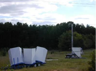
Figure Page 2.1 Environmental Protection Agency instrumentation cluster of three

trailers. In the foreground is the Model-2000 SODAR, further back is the Model 4000 miniSODAR and in the background is the 10- meter tower.

13

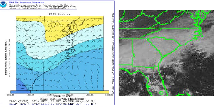
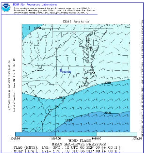
2.2 Eta Data Assimilation System (EDAS) analysis of sea- level pressure and surface wind (10 m), at 2000 LT (00 Z) on September 06, 2000 (Case 1).

17

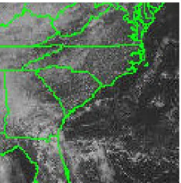
2.3 GOES-8 satellite image over the region showing deep cloud cover at 2000 LT (00Z) on September 06, 2000 (Case 1).

17

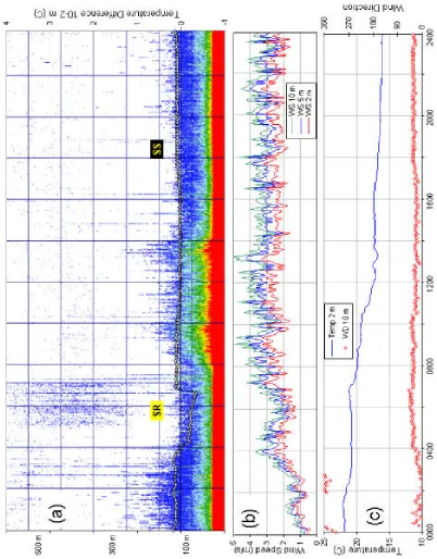
2.4 (Panel a) SODAR reflectivity from Model 2000 and tower measured 10-2 meter temperature difference (K) on September 6, 2001. SR

indicates sunrise and SS indicates sunset. (Panel b) Five minute averaged wind speed (m⋅s-1) at 2 m (red), 5 m (blue), and 10 m (green). (Panel c) Temperature (ºC) at 2 meters (blue) and wind direction (red).

18

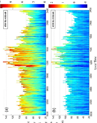
2.5 Velocity profile data from the Model 4000 miniSODAR on September 06, 2000. (Panel a) Horizontal wind speed (m⋅s-1), colors correspond to color bar to the right of the panel. (Panel b) Vertical velocity (m⋅s-1) for the same time period.

20

2.6 Eta Data Assimilation System analysis of sea-level pressure and surface wind (10 m) at 0800 LT (12 Z) on September 08, 2000 (Case 2).

2.7 GOES-8 satellite image over the region showing very little cloud cover at 1400 LT (18Z) on September 08, 2000 (Case 1)

22

2.8 (Panel a) SODAR reflectivity from Model 2000 and tower measured 10-2 meter temperature difference (K) on September 8, 2001. SR

indicates sunrise and SS indicates sunset. (Panel b) Five minute averaged wind speed (m⋅s-1) at 2 (red), 5 (blue), and 10 (green) meters. (Panel c) Temperature (ºC) at 2 meters (blue) and wind direction (red).

23

2.9

3.1

Velocity profile data from the Model 4000 miniSODAR on September 08, 2000. (Panel a) Horizontal wind speed (m⋅s-1), colors correspond to color bar to the right of the panel. (Panel b) Vertical velocity (m⋅s-1) for the same time period.

Plan view of the regional 6 km ARPS domain over central North Carolina. The location of the NC ECO Net surface observing stations are shown.

25

38

5.1 Figure 5.1 Plan view of the model domain with respect to India and the Arabian Sea.

46

5.2 ARPS vertical coordinate distribution for the tropical seabreeze case. 47

5.3 (a) X-Z cross-section of potential temperature and horizontal wind vectors at 500 LT, 24-hours from the model initialization. The x-axis is in kilometers with 0 km indicating the coastline (CL), negative distance is over the ocean. (b) Same cross-section as (a), but centered and magnified in on the land-sea interface.

5.4 (a) X-Z cross-section of potential temperature and horizontal wind vectors at 1000 LT, 29-hours from the model initialization. The x-axis is in kilometers with 0 km indicating the coastline (CL), negative distance is over the ocean. (b) Same cross-section as (a), but centered and magnified in on the land-sea interface.

51

5.5 (a) X-Z cross-section of potential temperature and horizontal wind vectors at 1400 LT, 33-hours from the model initialization. The x-axis is in kilometers with 0 km indicating the coastline (CL), negative distance is over the ocean. (b) Same cross-section as (a), but centered and magnified in on the land-sea interface.

53

5.6 (a) X-Z cross-section of potential temperature and horizontal wind vectors at 1900 LT, 38-hours from the model initialization. The x-axis is in 9ilometers with 0 km indicating the coastline (CL), negative distance is over the ocean. (b) Same cross-section as (a), but centered and magnified in on the land-sea interface.

55

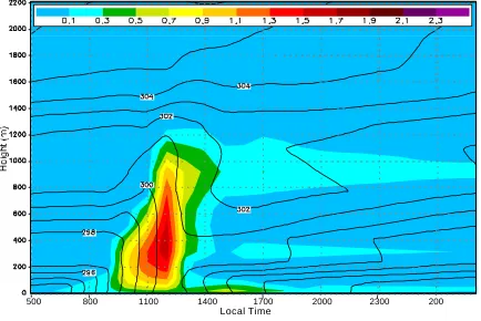
5.7 Time series profile of turbulent kinetic energy (TKE) and potential temperature at a location 5 km inland. Potential temperature is contoured each 1 degree and TKE (m^2/s^2) is shaded with legend shown.

56

5.8 Time series profile of turbulent kinetic energy (TKE) and potential temperature at a location 100 km inland. Potential temperature is contoured each 1 degree and TKE (m^2/s^2) is shaded with legend shown.

58

5.10 Concentration pattern of NOx from the various point sources. Blue shading represents the nighttime concentrations and red shading indicates the simulated daytime concentrations.

60

6.1 Regional view of North Carolina and the location of the 6 km ARPS model domain. Surface station (NC ECO Net) locations are depicted.

65

6.2 (a) Terrain height in meters and (b) soil type for the 6 km ARPS domain.

66

6.3 (a) Vegetation type and (b) surface roughness in meters for the 6 km ARPS model domain.

67

6.4 Eta Data Assimilation System (EDAS) analysis of sea level pressure gradient (mb) and 10 m wind (kt).

69

6.5 GOES-8 visible 1-km satellite image for the region on July 10, 2001 at 1500 LT.

70

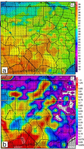
6.6 (a) Simulated 10 cm surface temperature (C) and 10 m wind vectors. (b) Simulated 100 m TKE (m^2/s^2) and 10 m wind vectors. Both panels are 8 hr forecast for July 10, 2001 at 1500 LT.

71

6.7 Advanced Very High Resolution (AVHRR) Satellite image showing surface skin temperature (C). (a) July 10, 2001 at approximately 1500 LT (b) July 11, 2001 near 1800 LT.

73

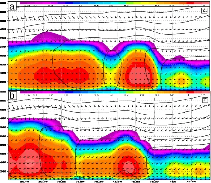
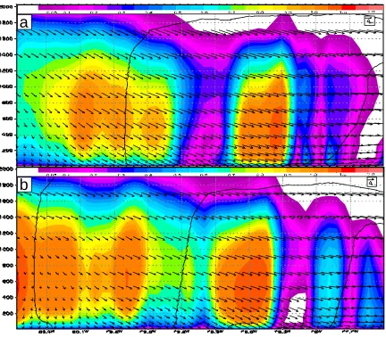
6.8 (a) Simulated vertical cross-section of potential temperature (contoured each 1 degree), TKE (m^2/s^2) and horizontal wind vectors for July 10, 2001 at 1500 LT for the upper cross-section. (b)

Same but for lower west-east cross section depicted in Figure 6.8b.

6.9 (a) Simulated 10 cm surface temperature (C) and 10 m wind vectors. (b) Simulated 100 m TKE (m^2/s^2) and 10 m wind vectors. Both panels are 33 hr forecast for July 11, 2001 at 1800 LT.

79

6.10 (a) Simulated vertical cross-section of potential temperature (contoured each 1 degree), TKE (m^2/s^2) and horizontal wind vectors for July 11, 2001 at 1800 LT for the upper cross-section. (b) Same but for lower west-east cross section depicted in Figure 6.8b.

80

6.11 (a) Simulated 10 cm surface temperature (C) and 10 m wind vectors. (b) Simulated 100 m TKE (m^2/s^2) and 10 m wind vectors. Both panels are 43 hr forecast for July 12, 2001 at 0400 LT.

82

6.12 (a) Simulated vertical cross-section of potential temperature (contoured each 1 degree), TKE (m^2/s^2) and horizontal wind vectors for July 12, 2001 at 0400 LT for the upper cross-section. (b) Same but for lower west-east cross section depicted in Figure 6.8b.

84

6.13 Observed and simulated 2 m temperature, 48 hr time series for all NC ECO Net stations.

86

6.14 Observed and simulated 10 m wind speed, 48 hr time series for all NC ECO Net stations.

90

6.15 Observed and simulated wind vectors, 48 hr time series for all NC ECO Net stations.

93

7.1 Plan view of high-resolution 1 km model domain over Raleigh, North Carolina. Major roadways, towns and the NC ECO Net station

locations are indicated.

7.2 Terrain and landuse properties over the Raleigh, North Carolina region as parameterized by ARPS.

100

7.3 (a) Simulated 10 cm surface temperature (C) and 10 m wind vectors. (b) Simulated 100 m TKE (m^2/s^2) and 10 m wind vectors. Both panels are for July 10, 2001 at 1500 LT.

102

7.4 Simulated vertical cross-section of potential temperature (contoured each 1 degree), TKE (m^2/s^2) and horizontal wind vectors for July 10, 2001 at 1500 LT for the upper cross-section.

104

7.5

7.5

(a) Simulated 10 cm surface temperature (C) and 10 m wind vectors. (b) Terrain height (m) and 10 m wind vectors. Both panels are for July 11, 2001 at 0500 LT.

(c) TKE (m2s-2) and potential temperature (each 1 K) vertical cross-section through the center of the 1 km model domain at 0500 LT on July 11th, 2001.

106

107

7.6 (a) Simulated 10 cm surface temperature (C) and 10 m wind vectors. (b) Simulated 100 m TKE (m^2/s^2) and 10 m wind vectors. Both panels are for July 11, 2001 at 1400 LT.

109

7.7 Simulated vertical cross-section of potential temperature (contoured each 1 degree), TKE (m^2/s^2) and horizontal wind vectors for July 11, 2001 at 1400 LT for the upper cross-section.

110

7.8 (a) Simulated 10 cm surface temperature (C) and 10 m wind vectors. (b) Terrain height (m) and 10 m wind vectors. Both panels are for July 12, 2001 at 0500 LT.

7.9 Aerovironment Model 2000 SODAR observed reflectivity (dB) for July 10, 2001 (0800 LT) to July 12, 2001 (0800 LT). Simulated potential temperature is contoured (K) each 1 degree for the corresponding period.

114

7.10 Aerovironment Model 4000 miniSODAR observed reflectivity for July 10, 2001 (0800 LT) to July 12, 2001 (0800 LT).

116

7.11 Simulated potential temperature (contoured 1 degree), TKE (shaded) and wind (kt) profile (upper). Aerovironment Model 2000 observed wind profile (kt) for July 10, 2001 (0800 LT) to July 11, 2001 (0800 LT).

118

7.12 Simulated potential temperature (contoured 1 degree), TKE (shaded) and wind (kt) profile (upper). Aerovironment Model 2000 observed wind profile (kt) for July 11, 2001 (0800 LT) to July 12, 2001 (0800 LT).

120

7.13 MicroFacPM simulated, diurnal PM2.5 concentration (g/km/hr) along Capital Blvd.

126

7.14 Simulated 1 hr average PM2.5 concentration (ug/m3) and 10 m wind

vectors at July 10th at 1000 LT.

128

7.15 Simulated 1 hr average PM2.5 concentration (ug/m3) and 10 m wind

vectors at July 10th at 1500 LT.

129

7.16 Simulated 1 hr average PM2.5 concentration (ug/m3) and 10 m wind

vectors at July 10th at 1800 LT.

131

vectors at July 10th at 2100 LT.

7.18 Simulated 1 hr average PM2.5 concentration (ug/m3) and 10 m wind

vectors at July 11th at 0200 LT.

133

7.19 Simulated 1 hr average PM2.5 concentration (ug/m3) and 10 m wind

vectors at July 11th at 0800 LT.

134

7.20 Simulated 1 hr average PM2.5 concentration (ug/m3) and 10 m wind

vectors at July 11th at 1800 LT.

135

7.21 Simulated 1 hr average PM2.5 concentration (ug/m3) and 10 m wind

vectors at July 12th at 0200 LT.

136

7.22 Simulated 1 hr average PM2.5 concentration (ug/m3) and 10 m wind

vectors at July 12th at 0700 LT.

LIST OF SYMBOLS

b Slope of the moisture retention curve of soil

1

C Coefficient of the net precipitation

2

C Coefficient of the perturbated near surface moisture content

d

C Surface exchange (drag) coefficient for momentum

g

C Thermal coefficient for bare soil

gsat

C Thermal coefficient for bare soil at saturation

h

C Surface exchange (drag) coefficient for heat

q

C Surface exchange (drag) coefficient of moisture

t

C Thermal coefficient for the surface

v

C Thermal coefficient for vegetation

g

E Evaporation from the ground

r

E Evaporation from the plant canopy

tr

E Transpiration

1

F Fractional conductance of photosynthetically active radiation

2

F Fractional conductance of water stress

3

F Fractional conductance of atmospheric vapor pressure

4

F Fractional conductance of air temperature

y

z

f Dimensionless time function in the vertical

w

F Wet fraction of the canopy g Gravitational acceleration

u

h Relative humidity at the ground surface H Sensible heat flux

k von Karman constant L Monin-Obukhov length

e

L Latent heat of evaporation LE Latent heat flux

η Length scale

0

η Length scale, scaled by the roughness length

a

ρ Air density

P Precipitation rate

g

P Residual of the precipitation rate at the ground

π 3.1415186

0

Pr Prandtl number

w

ρ Density of water q Specific humidity

s

q Specific humidity at the surface

v a

q Specific humidity at the first model level above the surface

vsat

a

R Aerodynamic resistance

g

R Short wave radiation at the surface

b

Ri Bulk Richardson number

n

R Net radiation at the surface

s

R Surface resistance to evapotranspiration

min

s

R Minimum of surface resistance

v

σ Horizontal fluctuation in velocity

w

σ Vertical fluctuation in velocity

yt

σ Time dependent dispersion coefficient in the crosswind direction

zt

σ Time dependent dispersion coefficient in the vertical direction

τ Length of day

θ Potential temperature

0

θ Potential temperature near the surface

s

θ Potential temperature at the surface

v

θ Mean virtual potential temperature in the surface layer

t Time

ty

t Time scale in the horizontal

tz

t Time scale in the vertical

2

T 10 to 100 cm soil temperature

s

T Surface to 10 cm soil temperature ' '

u Velocity component in x-direction

u* Friction velocity U Horizontal wind speed

V Velocity component in y-direction

V Mean wind speed at 10 m veg Vegetation percentage

*

w Convective velocity scale

w Velocity component in z-direction

2

W 10-100 cm soil moisture

g

W Surface to 10 cm soil moisture

geq

W Surface moisture when gravity and the capillary forces are balanced

r

W Canopy moisture

sat

W Soil saturation moisture ' '

wθ Kinematic heat flux

' '

w q Kinematic moisture flux

χ Similarity function

0

χ Similarity function scaled by the surface roughenss

z Height above the surface

i

z Boundary layer height

0

z Surface roughness

m

h

CHAPTER 1

INTRODUCTION

1.1 ATMOSPHERIC BOUNDARY LAYER AND AIR POLLUTION DISPERSION

Boundary layer meteorological processes are among the most important, fundamental aspects of atmospheric flow in relation to air pollution. The exchange and diffusion of heat, moisture, momentum, gases and particulates principally take place within the lowest kilometer of the troposphere. It is mainly the interaction between the atmosphere and earth’s surface that drives circulations from micro-scale up to global-scale.

Pollution sources, both man- made and natural, are in most cases near the earth’s surface within the atmospheric boundary layer. For this reason, boundary layer processes are essential in transporting, diffusing and diluting pollutants. Air pollution diffusion is controlled by several factors. Following a polluted parcel in the mean flow, turbulent fluctuations of the velocity will effectively cause the plume to expand in all directions as it is transported by the mean wind. These kinematic factors are the principal mechanisms that influence how pollutants emitted from a source are transported by the mean flow and diffused by turbulence.

An additional major factor that influences dispersion is the height of the boundary layer, sometimes referred to as the mixing height. This depth limits the vertical diffusion and therefore has a significant impact on boundary layer pollution concentrations. Lower boundary layer heights correspond to higher concentrations. The diffusion process becomes even more complicated in non-homogeneous boundary layers. Not considering synoptic scale systems, variations in the boundary layer can be directly related to changes in the surface characteristics. Hence, non- uniform surface features will result in complex variations of all the factors that affect pollution dispersion, ultimately leading to complex dispersion patterns.

How does the boundary layer vary over a sub-region and how do these small-scale variations influence the sub-regional to regional meteorological conditions and associated air quality? Can smaller scale boundary layer variations noticeably influence dispersion patterns?

topographically induce flows and others. It is known that small-scale heterogeneities related to the surface can create variations in the boundary layer structure. The surface variations examined in this thesis are those of topography, soil texture (type), soil moisture, surface roughness and vegetation cover.

Different soil types possess different physical properties and therefore heat and cool differently. Arya (2001) indicates that the thermal properties of soils depend on the solid particles, size distribution, porosity and moisture content. Gradients in soil types alone can cause gradients in surface heat and mo isture fluxes, thus gradients in the boundary layer properties. A study by Li and Avissar (1994) concluded that the influence of soil properties dominant the surface fluxes when ve getation cover is low.

Surface roughness is a function of the landuse. Forest areas with tall trees stimulate more resistance or friction to the flow when compared to an open field, lake or ocean. This in turn influences the amount of turbulent shear energy as well as the mean wind speed near the surface. Internal boundary layers can form due to sudden changes in roughness, wherein the vertical distribution of momentum and heat as well as surface fluxes will vary. Surface roughness has been noted in studies to influence the boundary layer structure most during neutral to stable stability regimes (Li and Avissar, 1994)

small-scale circulation, clouds and even precipitation in some cases. Bougeault et al. (1991) and Lyons et al. (1993) support this through both numerical modeling and observational studies.

Topography is another surface feature that can distinctly influence the boundary layer flow and turbulence. During stable, light wind conditions, a cooling surface in addition to the slope of a hill will cause the heavier cooler air to flow down the slope into the valley. Also, during strong statically stable conditions, hills can cause the flow to diverge around, rather than cross over the slope. Within a highly variable topographic locale, the boundary layer meteorology can be similarly as complicated.

Synoptic scale weather patterns present additional complexity in terms of the boundary layer properties affecting pollution dispersion. Active weather is more conducive to quick, efficient pollution dispersion and removal. Stronger wind leads to greater instability, turbulence and thus effective dilution. Stronger wind swiftly transports local pollutants away from the source region. Rainfall typically accompanies synoptic low-pressure systems, and can within hours remove a majority of pollutants through wet deposition.

from near-surface sources. Warm, statically stable air aloft limits the growth of the convective boundary layer and can therefore cause boundary layer concentrations to be higher. This coupled with clear skies during the day is a recipe for enhanced ozone production.

With all these factors considered, air pollution dispersion is strongly dependent on the spatially variable and non-stationary boundary layer meteorology. For this reason, dispersion models need comprehensive meteorology, which takes into account complex surface features that effect the boundary layer.

1.2 RESEARCH OVERVIEW AND OBJECTIVES

Additionally, the ARPS model simulations are statistically evaluated using surface observations from the North Carolina Environmental Climate Observing Network (NC ECO Net).

The U.S. Environmental Protection Agency, National Exposure Research Laboratory (EPA/NERL) has an instrumentation cluster that facilitates high- resolution temporal measurements near the surface. This ensemble consists of three portable trailers supporting an Aerovironment Model 4000 miniSODAR, Aerovironment Model 2000 SODAR and three- level 10 m micrometeorological tower. The emphasis here is on the diurnal structure of the surface layer using this observing system. Two 24 hr cases are inspected in which the meteorological conditions are dissimilar. The first observational period occurs during a high wind and deep cloud cover scenario; it is considered near neutral during both the daytime and nighttime hours. Conversely, little cloud cover and light wind govern the meteorology of the second case. For this case, the boundary layer is dominated by free convection during the day and strong thermal stability at night. An attempt is made to distinguish differences in the surface layer structure between two cases by examining the wind profiles, surface stability and SODAR observations.

turbulence and wind field is modified by this mesoscale circulation. Using simulated meteorological fields from the ARPS model, dispersion pattern from the CALPUFF model is examined along with boundary layer variations directly caused by air-sea interactions.

dispersion patterns from the ARPS-CALPUFF coupled simulation are evaluated for responses to variations in the boundary layer meteorology resulting from surface heterogeneities.

1.3 WHY COUPLE ARPS AND CALPUFF?

The CALPUFF modeling system is one of the more advanced dispersion models available and will soon be certified as a regulatory model of the United States Environmental Protection Agency (US EPA). CALPUFF has a micrometeorological module that takes in hourly surface observations, standard twice-daily upper-air observations and USGS land use land-cover information. From this data, using seve ral boundary layer parameterization schemes, the structure of the atmospheric boundary layer is estimated. Variables such as boundary layer height, Monin-Obukhov length, friction velocity and convective velocity scale are approximated from the surface and upper air data. As mentioned previously, a goal of this research is to bypass the diagnostic model (CALMET) used with CALPUFF and employ a more robust, physically sound, mesoscale model (ARPS) to obtain the required boundary layer variables.

Secondly, CALMET uses twice-daily upper-air soundings at 00 and 12 Z to calculate the vertical structure of the boundary layer. In the eastern United States, these soundings are taken in the morning and evening. Both are the times when the boundary layer is in a transitional state. Between the soundings, an equation is used to describe the heating and cooling within the boundary layer using the hourly-observed surface temperature. In many cases this cannot accurately describe the actual evolution of the boundary layer. In addition, upper-air observations are sparsely spaced across the continental United States. If one is interested in smaller-scale dispersion, for example a city scale domain, it will be difficult to have a rawindsonde station within or even near the domain. For example, a CALMET domain set up over Raleigh, North Carolina would use the upper-air observations from Greensboro (~150 km) and Morehead City (250 km) to quantify the boundary layer. ARPS on the other hand uses the assimilated data, which includes these upper-air observations, radar, satellite, surface as well as model data.

CALMET uses wind observations to objectively derive the spatial and temporally varying wind field within the model domain. In many cases, especially when smaller scale simulations are of interest, few surface observations are available. For this reason, it is not possible to simulate smaller scale circulations such as seabreeze systems, landuse induced circulations and topographically influenced flows. ARPS has the physical equations that more realistically simulate these smaller scale features.

similar information along with an equation for the surface energy balance to derive the surface heat flux. Cloud-cover is used from the surface observations to estimate the incoming solar radiation, which in many cases is not available. The net radiation at the surface in combination with a specified Bowen ratio and a ground heat flux parameter is used for this heat flux estimation. Soil moisture is indirectly included as a constant Bowen ratio term for each landuse category. In ARPS the soil moisture is explicitly forecasted, which allows for changes during the simulation. Also, initial values of soil moisture from the ARPS Data Assimilation System (ADAS) analysis takes into account precipitation history. In short, the ARPS model is more physically advanced.

1.4 RESEARCH LAYOUT

CHAPTER 2

SODAR AND TOWER OBSERVATIONS

2.1 OVERVIEW

Instruments including SOund Detection And Ranging (SODAR), Light Detection and Ranging (LIDAR), towers, tetroons, and others allow probing of the lower atmosphere, the planetary boundary layer (PBL). The U.S. Environmental Protection Agency, National Exposure Research Laboratory (EPA/NERL) has an instrumentation cluster that facilitates high-resolution temporal and spatial measurements close to the surface. This consists of three portable trailers (Figure 2.1) supporting an Aerovironment Model 4000 miniSODAR (SOund Detection and Ranging), Aerovironment Model 2000 SODAR and three- level micrometeorological tower.

It is well known that when the boundary layer is stable, typically at night, wind speed increases with height to the top of the nocturnal boundary layer. The height of the nocturnal boundary layer is often associated with a core of high winds, a nocturnal jet (Stull, 1988). During near-neutral conditions the wind profile has a logarithmic distribution with height in the lower part of the planetary boundary layer, called the surface layer. Unstable conditions (convective), with light wind and high insolation situations yield a rapidly increasing wind speed in the shallow surface layer and near constant wind speed profile in the mixed layer.

meteorology dominates. Routine National Center for Environmental Prediction (NCEP) models provide gridded meteorological data for the entire United States, but the resolution of this data is not sufficient for determining local meteorology for the support of small scale pollution modeling. Similarly, routine meteorology measured at airports or other stations is only representative of the surrounding area. The EPA/NERL cluster of instruments is being used to support site-specific field studies of human exposure to pollutants. These measurements of local meteorology near the surface are used to develop and evaluate a local scale meteorological modeling system for general application in

Figure 2.1 Environmental Protection Agency instrumentation cluster of three

support of human exposure modeling. Air quality and consequently exposure of humans will be affected by the local meteorology.

This section of the thesis presents observation from a field site near EPA's facilities in Research Triangle Park, North Carolina. The focus at this point is on the diurnal structure of the surface layer using the observing systems. An attempt is made to distinguish differences in the surface layer structure between three stability regimes and make qualitative comparisons with various boundary layer theories.

Observations are analyzed where the meteorological conditions are extremely unstable or convective during the day (Pasquill’s stability class A) and weakly to moderately stable at night (Class E-F). These stability classes are defined and widely used in air quality models (Arya, 1999). In addition, a case is examined where the day and night stability is near neutral (Class D), i.e. a cloudy-windy scenario (Stull, 1988). The observational analysis includes SODAR velocity profiles, 10-2 m temperature different ial (?T10m-2m), 2 m temperature, 10 m wind speed and direction and SODAR

reflectivity (digital facsimile).

A description of the two SODARs, 10 m tower, and site layout is given in the following section. Observations for two 24-hr periods will be analyzed and discussed with one near- neutral case and another with convective boundary layer during the day and stable boundary layer at night.

2.2 INSTRUMENTATION AND DATA DESCRIPTION

Hz, which mitigates environmental noise interference (Crescenti, 1998), leading to a better representation of the surface layer wind distribution and variance. A previous study evaluating the performance of ground based meteorological instruments including the same miniSODAR found a high correlation with tower measurements (Crescenti, 1999).

SODAR systems use sound to sample the boundary layer, emitting a pulse and receiving reflections from small gradients of temperature and moisture. Turbulent mixing is the main cause for these gradients. Frequency shifts (Doppler effect) from the transmitted to returned signal are translated as moving parcels of air, where the velocity is directly related to the frequency shift. Algorithms extract other related parameters such as standard deviations of the wind components, vertical velocity, and return signal intensity (reflectivity). The standard deviations provide useful information on the turbulence intensities while the return signal intensity may be used to distinguish mixing layers, both of which are important factors in air pollution dispersion.

An additional SODAR unit, Aerovironment Model 2000 SODAR, measures these same wind properties from 60 to 600 m at 30 m intervals, and averaged over a 10 minute period. This unit provides important data from the convective mixed layer, verifies the performance of the miniSODAR, and gives boundary layer heights when below 600 m. Additionally, the boundary layer height evolution after sunrise and before sunset can typically be assessed with this unit.

providing the lower level observations not sampled by either SODAR. The temperature observations, especially the difference between 2 and 10 m, provide valuable information on the static stability of the surface layer. All tower data are sampled each second then averaged and stored at 5 min intervals.

The observation site is located in Research Triangle Park, NC at a site called Jenkins Road. SODAR instrumentation was positioned in the center of an open field surrounded by 10 to 15 meter trees, at least 100 m away in all directions. The surrounding forest dampens the ambient noise level; this allows less interference and therefore more reliable SODAR data (Crescenti, 1998). The micrometeorological tower was located 3 km to the east with very similar surroundings.

2.3 OBSERVATION ANALYSIS

Two case analyses are offered below. For the first case (near- neutral case on September 06, 2000), diurnal 10 m wind speed remained strong (averaged 3 to 4 m⋅s-1) and constant through most of the period. The diurnal temperature range was small, less than 5° C, while the difference in temperature between 2-10 m was near zero.

2.3.1 NEAR-NEUTRAL CASE (SEPTEMBER 06, 2000)

The near- neutral case occurred during a cold air-damming event. These occurrences are characterized by strong surface high pressure developing over New England resulting in brisk north-northeast wind over the Mid-Atlantic States. As a result, cool Maritime polar air from the North Atlantic is transported into the region. Figure 2.2 provides the ETA analysis (EDAS) for 2000 LT (0000 UTC), which includes sea- level pressure (shaded) and 10 m wind. Typically, a warm- moist southwesterly flow overrides the cooler air at the surface. The result is cool, breezy, and cloudy weather. Figure 2.3 shows a visible satellite image at 1800 LT on this day, in which deep cloud cover envelops the region.

Figure 2.4(a) presents the digital facsimile analysis (DFS) for this case as seen by the Model 2000 SODAR. The surface layer (SBL) remains at a constant depth of 100 m for the 24-hour period. At night strong shear production overcomes negative buoyancy,

Figure 2.2 Analysis of sea- level pressure and surface wind (10 m) at 2000 LT (00 Z) on September 06, 2000 (Case 1:neutral).

Figure 2.3 GOES-8 satellite image over

resulting in a near neutral flow. During the daytime little change takes place because heavy cloud cover and limited solar insolation does not allow the surface to heat. In

Figure 2.4(a) SODAR reflectivity from Model 2000 and tower measured 10-2 meter temperature difference (K) on September 6, 2001. SR indicates sunrise and SS

addition, brisk winds kept the surface layer well mixed. These types of cloudy, windy conditions typically cause the surface layer to remain near neutral (Stull, 1988).

The SODAR reflectivity (Figure 2.4a) is consistent with near- neutral conditio ns. Evenly distributed echoes are a result of uniform small-scale temperature and specific humidity gradients that reflect sound wave signals back to the SODAR receiver. It is possible that humidity gradients may be a key source of the sound reflections. On this day, the soil moisture was high (0.33 m3⋅m-3) and it appears that cold/dry air advection took place. This sets up a stronger than normal moisture gradient near the surface.

Temperature gradient between 2 m and 10 m (?T10m-2m) is plotted on the digital

facsimile plot (Figure 2.4a). This vertical temperature gradient provides a measure of static stability. Temperature difference between the two levels remains close to zero for the 24-hr period, further suggesting a near-neutral surface layer.

Tower wind speed measurements in Figure 2.4b, indicate an increase in wind speed at 0300 LT from 1.5 to 4 m⋅s-1. At the same time, the near surface temperature difference (Figure 2.4a) transitions from slightly stable to slightly unstable. It is believed that the cold air advection is initiated at this time as a cool front passed through the region. Figure 2.4c gives the 2 m temperature time series along with the wind direction. The air temperature variation supports cold air advection and cool frontal passage. After the cool front passes (0300 LT) the temperature declines through the remainder of the day. Steady northeasterly wind direction was present for the whole period.

bursts of momentum correspond to strong boundary layer eddies formed by shear stress with the surface. In general, the increase in wind speed with height is uniform during the

Figure 2.5 Velocity profile data from the Model 4000 miniSODAR on

period. Figure 2.5b shows the vertical velocity measured from the miniSODAR for the same case. An interesting correlation exists between the horizontal wind speed in Figure 2.5a and the vertical velocity in Figure 2.5b. At the same points in time where the horizontal wind speed increases, the vertical velocity becomes negative. This indicates that the bursts of wind are associated with downward motion or a transfer of momentum downward. Boundary layer momentum flux, from higher to lower (down gradient transfer), is what these observation are explicitly showing.

2.3.2 CONVECTIVE CASE (SEPTEMBER 08, 2000)

Case 2 occurred on a day when the wind speed was light and solar insolation not hampered by cloud cover. Figures 2.6 and 2.7 present the sea level pressure, 10 m wind and a satellite image at 1800 LT. Both figures confirm the description of the meteorology

for this case. These types of conditions are conducive for a convective boundary layer where buoyancy driven turbulence dominates.

Figure 2.8a shows the digital facsimile analysis (DFS) from the Model 2000 SODAR. Between midnight and approximately 0615 LT the temperature difference corresponds to a slightly stable surface layer (dotted line overlaid on DFS). The DFS data indicates the stable nocturnal boundary layer height decreasing from 150 m to 120 m. After sunrise (0800 LT) the static stability becomes unstable in response to surface heating. At this point, the boundary layer begins an exponential growth. By 1000 LT the boundary layer height is above SODAR detection and the PBL becomes convective. It is noticed that strong surface layer thermals periodically arise, similar to convective SODAR data presented by Gera and Saxena (1996). The reflectivity, much greater than

Figure 2.7 GOES-8 satellite image over the region showing very

the previous neutral case, is indicative of intense temperature gradients within these thermals. The periodic decrease in the ? T10m-2m corresponds well with the intense

Figure 2.8(a) SODAR reflectivity from Model 2000 and tower measured 10-2

SODAR echoes. Around 1800 LT the static stability transitions to stable once again. At this point, the boundary layer quickly collapses to around 130 m. It is worth noting that some echoes remain above the boundary layer after sunset. These are believed to be diminishing turbulence in the residual layer.

Tower wind speed measurements, shown in Figure 2.8b, have periodic variation throughout the day. It appears that the sharp changes in wind speed may be related to the convective thermals. Near sunset, when the boundary layer collapses (1800 LT), wind speed diminishes, as does the variation in wind speed.

The temperature time series (Figure 2.8c) shows a typical diurnal variation where little cloud cover exists. Temperature decreases through the night, reaches a minimum at 0615 LT and then increases in response to surface heating, reaching a maximum in the afternoon and then decreases just before sunset. The wind direction shows more variability during the day compared to the evening and nighttime periods.

above the surface near the top of the stable boundary layer. During the day when the boundary layer is convective, the variation in vertical velocity is high. Strong upward

Figure 2.9 Velocity profile data from the Model 4000 miniSODAR on

motion (0.5-1.5 m⋅s-1) corresponds to the periodic thermals, followed by periods of weak decent (-0.5 m⋅s-1).

2.4 SUMMARY

The main emphasis of this chapter is to compare and contrast boundary layer observations from the instrument cluster during two typical meteorological conditions. The presented observational analysis does show a significant difference between the two cases. The near- neutral case showed that the boundary layer properties remained relatively constant during the 24- hour observational period. The SODAR reflectivity indicated that the surface boundary layer height remained around 100 m in which the echoes were strong and nearly uniform. The stability, implied from the 10-2 m temperature difference, supports a near- neutral boundary layer.

Chapter 3

ADVANCE REGIONAL PREDICTION SYSTEM (ARPS)

ARPS is the model elected for the mesoscale meteorological simulations and coupling with the CALPUFF dispersion model. In this chapter, information on ARPS, how it was used and configured is discussed. These details include general model characteristics, parameterizations employed and the land-surface as well as the turbulent flux numerical schemes. In addition to the ARPS details, a discussion is included on how the model data was used for CALPUFF. A brief discussion on the surface data used to validate the model performance is also included.

3.1 OVERVIEW OF THE ARPS MODELING SYSTEM

as a number of output formats for various popular environmental visualization software (Grads, Vis-5D, etc). In addition to these features, the ARPS model contains a preprocessing code to assimilate a variety of observations including atypical WSR-88D radar, wind profiler and satellite data.

ARPS is a non- hydrostatic, fully compressible primitive equation model appropriate for scales ranging from meters to kilometers (Xue et. al. 1995). The vertical coordinate system is a generalized terrain following coordinate with options for stretched or equal spacing while the horizontal grid spacing is equal in both the x and y directions. Additional grid options are included for 1-D, 2-D or 3-D simulations. Prognostic variables include 3-D wind components, potential temperature, pressure, sub- grid scale TKE and moisture related variables (specific humidity, cloud water, cloud ice and even hail/graupel).

3.2 NUMERICAL DETAILS

3.2.1 INTEGRATION, SMOOTHING, TKE CLOSURE AND RADIATION

option. Spatial derivatives are estimated using 2nd order accurate finite difference except for advection terms, which are 4th order accurate. Computational smoothing is employed so that numerical noise is dampened. In these simulations a 4th order mixing coefficient is used in both the vertical and horizontal direction.

Turbulence closure was realized through 1.5-order TKE turbulence closure following the non- local scheme of Sun and Chang (1986). In this scheme a budget equation for subgrid scale TKE is solved which includes buoyancy, shear production, advection (diffusion and transport) and viscous dissipation. Moist processes are explicitly considered along with the Kain and Fritsch cumulus parameterization (Kain and Fritsch, 1993). Radiation physics are simulated using atmospheric radiation transfer parameterization developed at NASA/Goddard Space Flight Center and tailored for ARPS. This scheme includes equations for both short wave (Chou, 1990; Chou, 1992) and long wave (Chou and Suarez, 1994) radiation processes. Additional details related to the formulations can be found in Xue et al. (1995), Xue et. al. (2000) and Xue et. al. (2001).

3.2.2 SURFACE FLUXES AND LAND-SURFACE MODEL

ARPS uses surface roughness and a stability dependent surface flux model first developed by Businger et. al. (1971) then modified by Deardorff (1972b), in order to account for extremely stable and unstable situations. The surface fluxes considered are: momentum (Eq. 3.1 and 3.2), heat (Eq. 3.3) and moisture (Eq. 3.4). The stability dependent drag coefficient of momentum (Cd) along with the first leve l (10 m) wind

speed (V) and wind components (u,v) are used to calculate the momentum flux. Similarly, the heat flux is calculated using the stability dependent drag coefficient of heat (Ch), first

level wind speed and the temperature difference (θ θ− _s) between the ground and first level (10 m) above the surface. The same method is used for the moisture flux with the difference in specific humidity

(

)

' ' _d

u w = −C Vu (3.1)

' ' _d

v w = −C Vv (3.2)

(

)

' ' _{h s}

wθ = −C V θ θ− (3.3)

(

)

' ' q s

w q = −C V q q− (3.4)

The Deardorff scheme first determines the stability near the surface. Stability is determined using the bulk Richardson number (Rib), which follows the form of Eq. 3.5.

from the 14 categorized vegetation type assigned by the world ecosystem class data (Kineman and Ohrenschall, 1992).

0 2 0 ( ) b z z g Ri U θ θ ∆ −

= (3.5)

2

2 0

0

[ln( ) ( , )]

d m k C z z z

z ψ L L

= − (3.6) 2 0 0 0 0 0

[ln( ) ( , )][Pr (ln( ) ( , ))]

h

m h

k C

z z

z z z z

z ψ L L z ψ L L

=

− −

(3.7)

1 2 2 1 1 1

0 0 0

2ln[(1 )(1 ) ] ln[(1 )(1 ) ] 2tan 2tan

m

ψ _{= +}χ ₊χ − _{+ +}χ ₊χ − ₋ − χ₊ − χ _(3.8)

1 0

2ln[(1 )(1 ) ]

h

ψ _{= +}η ₊η − _(3.9)

During neutral stability conditions the exchange coefficients are calculated using the same equations with an extremely small, negative bulk Richardson number. When the stability is exceedingly unstable or free convective, Deardorff’s (1972b) method uses the minimum of the unstable calculated value or double the neutral value. Similarly, the exchange coefficient of heat is determined during convective conditions as the minimum of the unstable calculated value or 3.33 times the neutral value. Stable situations are treated different but also take after Deardorff (1972b). The general idea is to scale the

neutral values of both the heat and momentum drag coefficient by 1 b c Ri Ri   −  

 . Where Ric is

Important to the stability determination and the heat and moisture fluxes is the soil state. The soil- vegetation model from Noilhan and Planton (1989) is employed by ARPS to predict how the soil temperature, moisture and canopy moisture varies spatially and temporally. The following five equations show how these calculations are executed. Eq. 3.10 relates the change in surface temperature, defined as the upper 10 cm, to ground heat flux

(

)

layer below (T2). Eq. 3.11 solves the change in deep soil temperature as a function of the

soil temperature above. Near surface soil moisture (Wg) changes are defined (Eq. 3.12) as

a function of precipitation reaching the ground and dew formation (Pg), direct evaporation

(Eg), flow to lower soil levels (Wg −Wgeq) and runoff (Rg). Coefficients C1 and C2 are

dependent on the soil type, saturation and layer depth.

(

)

2

( )

s

t n s

T

C R H LE T T

t π τ ∂ = − − − − ∂ (3.10) 2 2 1

( _s )

T T T t τ ∂ = − ∂ (3.11)

(

)

g g g geq g

w

W C C

P E W W R

t ρ d τ

∂

= − − − −

∂ (3.12)

(

)

2

2

1

g g tr

w

W

P E E

t ρ d

∂ _{= − −}

∂ (3.13)

( )

r

r

W

veg P E t

∂ _{= −}

∂ (3.14)

Eq. 3.13 is for the time dependent change in deep soil moisture (W2) is similar in

(d2). Canopy moisture (Wr) is also solved as a function of vegetation percentage (veg),

precipitation (P) and canopy evaporation (Eg) as shown by Eq. 3.14.

Important to many of the land-surface calculations is the classification of the surface. ARPS defines the surface by the following parameters: soil type, vegetation type, vegetation fraction (veg), leaf-area index (LAI) and surface roughness (zo). Soil types are

specified with different thermal and moisture retention properties. These directly influence the heating/cooling rate of the surface. The soil type classification includes 13 categories and comes from the State Soil Geographic (STATSGO) archive (NSSC, 1994). Vegetation percentage becomes an important factor in determining the bulk thermal coefficient (Ct) of the surface, which includes the effect of both the soil and vegetation

thermal properties. The vegetation percentage is derived from the Normalized Difference Vegetation Index (NDVI) corresponding to satellite observations (Kidwell, 1990). Equations 3.15 and 3.16 outline this approach, where Cv is a constant thermal coefficient

of vegetation, Cg is the therma l coefficient for the soil type and Cgsat is the same for the

soil when saturated. 1 1 t g v C veg veg C C = ₋ + (3.15) (2ln10) 2 b sat g gsat W C C W   = _{ }

  (3.16)

Evaporation from the surface (Eg), vegetation transpiration (Etr) and the plant

a sum of these processes (Eq. 3.17). Equations for the various evaporation parameters used in the model are outlined in Eq. 3.18 to 3.20.

( )

e g tr r

LE=L E +E +E (3.17)

(1 ) [ ( ) ]

g a q u vsat s va

E = −veg ρ C V h q T −q (3.18)

1

[ ( ) ]

w

tr a vsat s va

a s

F

E veg q T q

R R

ρ −

= −

+ (3.19)

[ ( ) ]

w

r a vsat s va

a

F

E veg q T q

R

ρ

= − (3.20)

Leaf area index is another important surface characteristic in terms of the influence on evaporative and radiative processes. LAI is involved in calculating the resistance of the surface to evapotranspiration, which is defined by Rs (Eq 3.21). The LAI

is derived from the same NDVI database as the vegetation percentage. For further clarification, the ARPS Users Guide gives in depth details on how some of the unexplained coefficients are estimated.

min

1 2 3 4

( )

s s

R R

LAI F F F F

= (3.21)

3.3 INITIALIZATION AND BOUNDARY CONDITIONS

sounding. These options allow for idealized simulations including density currents (Xue et. al., 1998), storm cells, and seabreeze fronts (Gilliam et. al., 2001). Other options allow ARPS to be initialized using more realistic data from many of the available operational models including Aviation Model (AVN), ETA, Rapid Update Cycle (RUC), ARPS and COAMPS data. This research takes advantage of both the idealized single sounding initialization and the realistic initialization using the 32 km ARPS model analysis provided by the CAPS group.

Boundary conditions (BC) are necessary for all limited domain models. In ARPS, five options are available for lateral boundary conditions. These include wall BC, periodic BC, zero gradient BC, open (radiative) BC and external BC from another model. In this study, the zero gradient BC was used for the seabreeze simulation over the Mumbai, India region. This option involves setting the outer grid point values equal to the adjacent inner grid point. For the realistic 6-km simulations over Eastern North Carolina, external boundary conditions were provided by and extracted from the ARPS Data Assimilation System (ADAS). For the 1-km simulations over Raleigh, the 6-km simulation provides initialization and boundary conditions. An ARPS preprocessing program ext2arps extracts the values of the prognostic variable at specified time intervals for the outer edges of the grid domain. A linear interpolation is performed between the extracted time periods so that boundary condition values are available for each time step. For more details on the specifics of these numerical methods, refer to the ARPS Users Guide.

In order to successfully couple ARPS with CALPUFF several boundary layer properties need to be either extracted or calculated from the simulated meteorology. The meteorological fields required by CALPUFF are wind components (u,v,w), potential temperature at all levels, friction velocity, Monin-Obukhov length, convective velocity scale and mixing height. ARPS standard output directly provides some of these meteorological parameters but several were derived. Variables such as the wind, potential temperature and friction velocity were directly extracted; however, the boundary layer height, Monin-Obukhov length and convective velocity scale were either diagnosed or calculated using other available variables. A conversion program in FORTRAN was written to convert the hourly ARPS output and derive unavailable variables, into a format appropriate for CALPUFF.

Mixing height was calculated using the turbulent kinetic energy (TKE) profile. Stull (1988) provides several well-known methods for determining the height of the planetary boundary layer (PBL). By definition, the PBL is the layer affected by the earths surface and hence, a turbulent layer. Vertical TKE distrib ution, in theory, describes the extent of the PBL. The PBL height needed by CALPUFF is derived from ARPS as the height where the TKE drops to less than 5% of the maximum value in the boundary layer (Stull, 1988). The diagnostic algorithm looks at the simulated TKE profile, finds the maximum value in the boundary layer for each grid cell and then finds the height where this maximum value decreases to 5%. Using the analyzed mixing height (zi), surface

convective velocity scale, friction velocity (u*) and potential temperature are used to

calculate the Monin-Obukhov length (L) according to Stull (1988) as in Eq. 3.23.

( )

' ' * i v s v gz

w wθ

θ

 

=  

  (3.22)

(

)

3 *

' _v'

s v

u L

g

k wθ

θ

= − (3.23)

3.5 SURFACE OBSERVATIONS

prediction for a variable like wind speed at a specific grid point, is a volume average not a point measurement like observations. For this reason, the comparison between observed and predicted variables should not be exact but have differences, which are a function of using finite-difference methods to solve fluid motion equations. However, the comparison should yield similarities in both magnitude and trend. The simulated and observed data will be compared using both time series plots over the simulation period and a more quantit ative analysis using typical model performance statistics.

gives an idea of the distribution of differences between observed and predicted. Eq. 3.26 shows how the root mean square error is calculated. The mean average error is calculated according to Eq. 3.27 and Eq. 3.28 shows the idex of agreement.

1

1 N

i i

i

MBE P O

N ₌

=

∑

1 2

1

( 1) ( )

N

i i

i

VAR N − P O MBE

=

= −

∑

0.5 1 2 1 ( ) N i i i

RMSE N− P O

=

 

=_ − _



∑

1

1

N

i i

i

MAE N− P O

=

=

∑

(

) (

)

P O O O

CHAPTER 4

CALPUFF MODELING SYSTEM

In this chapter some details of the CALPUFF dispersion modeling system are given. These include information on how the dispersion coefficients are derived from the meteorological fields, various source types used in this study and some other model information.

4.1 BACKGROUND

It is generally recognized that CALPUFF, a non-steady state Gaussian plume model, out-performs many other available dispersion models including Industrial Source Complex 3 (ISC3) and Mesoscale Puff (MESOPUFF) (Allwine, Dabberdt, and Simmons, 1998). Simpler dispersion models only allow spatially constant conditions (steady state) and therefore, perform rather poorly during light wind and non-homogeneous conditions. Many of these models also assume homogeneous and constant surface characteristics. Since most air quality problems occur during variable meteorological conditions, CALPUFF has potential to provide more accurate estimations of huma n exposure to environmental pollutants for any given representative meteorological conditions.