ABSTRACT
GAVASKAR, NILESH RAMESH. A Framework for Performance Analysis of Virtual Collaborative Environments. (Under the direction of Michael Devetsikiotis.)
c
Copyright 2010 by Nilesh Ramesh Gavaskar
A Framework for Performance Analysis of Virtual Collaborative Environments
by
Nilesh Ramesh Gavaskar
A thesis submitted to the Graduate Faculty of North Carolina State University
in partial fulfillment of the requirements for the Degree of
Master of Science
Computer Science
Raleigh, North Carolina
2010
APPROVED BY:
Do Young Eun Laurie Williams
DEDICATION
BIOGRAPHY
ACKNOWLEDGEMENTS
I would like to express sincere gratitude towards Dr. Michael Devetsikiotis for giving me an opportunity to work with him and for his constant guidance in my research work. I would also like to thank Dr. Do Young Eun and Dr. Laurie Williams for expressing interest in my work and for serving on my thesis committee.
I would like to express special thanks to Dr. Michael Kallitsis for this insightful suggestions and his valuable support towards my thesis. I would also like to thank all my friends and colleagues: Kauti, Mihir, Nadu, Ritesh, Sreekanth, Vikas, Kedar, Santhosh, Deepak, Ashwin, Shrikant, Pradeep, Deepti, Keerthana, Yan and Ioannis for a fun-filled and a memorable two year journey towards my Masters degree.
TABLE OF CONTENTS
List of Tables . . . vii
List of Figures . . . viii
Chapter 1 Introduction . . . 1
1.1 Overview . . . 1
1.2 Motivation . . . 2
1.3 Introduction to Virtual Worlds . . . 3
1.3.1 Avatars . . . 4
1.3.2 Presence: The In-World Factor/Feeling . . . 4
1.3.3 OpenSimulator . . . 6
1.3.4 The Wonderland environment . . . 6
1.4 Contribution . . . 7
1.5 Related Work . . . 9
1.6 Thesis Organization . . . 10
Chapter 2 The Wonderland-Matlab experiment . . . 11
2.1 Introduction . . . 11
2.2 Objective . . . 12
2.3 Experiment Design . . . 12
2.3.1 The Matlab test . . . 14
2.3.2 Experiment monitoring setup . . . 14
2.3.3 Survey . . . 16
2.4 Summary . . . 17
Chapter 3 The OpenSim Experiment . . . 18
3.1 Introduction . . . 18
3.2 OpenSim Configuration servers . . . 19
3.2.1 Core Server . . . 19
3.2.2 Voice Server . . . 20
3.3 Overview of the World . . . 20
3.4 The Maze . . . 21
3.4.1 The Maze Automation scripts . . . 21
3.4.2 Integration of voice . . . 23
3.4.3 Automating the experiment with bots . . . 23
3.4.4 The SQLite Database . . . 25
3.5 Varying the control parameters . . . 25
3.5.1 Simulation of the communication between participants . . . 25
3.5.2 Bandwidth variation . . . 27
3.5.3 CPU load variation . . . 29
Chapter 4 Metamodelling: Framework and Case Studies . . . 30
4.1 Introduction . . . 30
4.1.1 Introduction to metamodelling . . . 30
4.2 The Metamodelling methodology . . . 31
4.2.1 Design of the experiment . . . 33
4.2.2 Choosing an appropriate model . . . 33
4.2.3 Fitting the model . . . 34
4.3 Problem Formulation . . . 34
4.3.1 Problem Statement . . . 34
4.3.2 Inputs . . . 35
4.3.3 Outputs . . . 36
4.4 Case Studies . . . 36
4.4.1 Case Study 1: The maze with textual message traffic . . . 37
4.4.2 Case Study 2: The maze with voice communication traffic . . . 39
4.5 Optimum Allocation of Resources . . . 43
4.5.1 Cost Functions . . . 46
4.5.2 Optimization Problems . . . 47
4.6 Performance Evaluation . . . 47
4.7 Summary . . . 48
Chapter 5 Conclusion . . . 49
5.1 Summary . . . 49
5.2 Future work . . . 51
5.2.1 Conducting the experiments with human subjects . . . 51
5.2.2 Resource optimization with the marketing point of view . . . 51
5.2.3 Analysis of the VCE with actual voice transmissions . . . 51
References . . . 52
Appendix . . . 55
Appendix A . . . 56
A.1 Configuring the OpenSim core server . . . 56
A.2 Configuring the OpenSim voice server . . . 58
A.3 Scripting code - Opensim . . . 59
A.3.1 LSL example code snippets . . . 59
LIST OF TABLES
Table 4.1 Bots to % CPU transformation . . . 35
Table 4.2 Case 1: Chat Message Commands . . . 39
Table 4.3 Case 2: Using voice command simulation . . . 42
Table 4.4 Results for time minimization . . . 48
LIST OF FIGURES
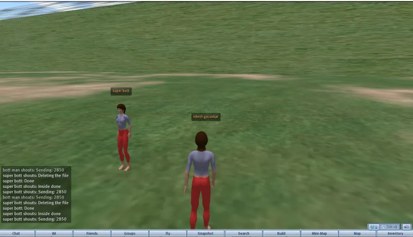
Figure 1.1 The image shows us what an avatar looks like inside the virtual world SecondLife 5 Figure 1.2 The image above gives us a glimpse of the wonderland world. We can see two
avatars standing in front of the screen with the matlab exercise. . . 7
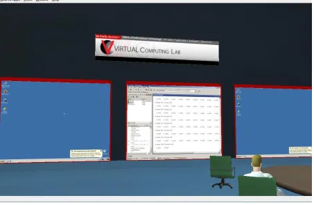
Figure 2.1 Here we see three VNC screens embedded inside the virtual world. . . 13
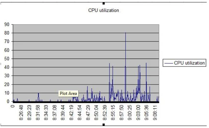
Figure 2.2 The CPU utilization measurements . . . 15
Figure 2.3 The network utilization graph . . . 15
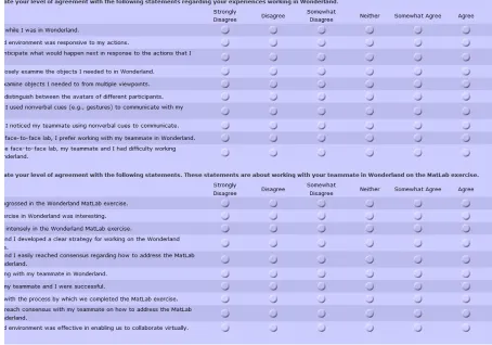
Figure 2.4 The survey questionnaire . . . 16
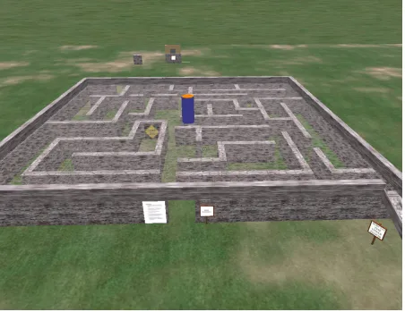
Figure 3.1 Here we see a picture of experimental maze from the front . . . 22
Figure 3.2 The image shows us the path a packet follows through theNetfilterhooks . . . . 28
Figure 4.1 Sending messages and receiving acknowledgements . . . 38
Figure 4.2 Linear response surface for chat communication . . . 40
Figure 4.3 Non-linear response surface for chat communication . . . 41
Figure 4.4 Linear response surface for chat and voice communication . . . 44
Figure 4.5 Non-linear response surface for chat and voice communication . . . 45
Figure A.1 Distance calculator code snippet . . . 60
CHAPTER
1
Introduction
1.1
Overview
Virtual spaces like these are also regarded as collaborative working environments. Unlike voice and video conferences, these enable perception of the surrounding individuals as tangible entities inside the virtual workspace. They thus provide capabilities to share information such as desktop along with the provision of traditional video/voice communication. This thus enables a shift of paradigm from the traditional geographical collocation or the proximity paradigm to the virtual collocation ideology where professionals collaborate with one another regardless of their geographical location.
Social presence inside such worlds is a big factor in determination of a world being enjoyable and feeling real. One may define presence inside an environment as the ability of the domain to make its users feel comfortable and truly inside it. The inhabitants need to be able to immerse themselves into the world and feel like they are a part of it. Virtual presence which is a parallel term for virtual environments, is thus one of the key factors which can help us determine the level of user experience and acceptability of these environments.
1.2
Motivation
Combined with the the high potential encompassed by these virtual spaces for social interaction, the computing and networking needs of these arenas are also growing at an accelerated pace. It is thus necessary for us to be proactive in optimizing the processing power and networking assets at hand while making sure that we do not compromise on the social networking aspect of these work spaces. A small change in the computing parameters can spoil or enhance the user experience. The kind of objects the user interacts with inside the world and the quality of their depiction can change the way a student understands a remotely taught lesson. Analysis of the social aspect of this problem adds a new facet to the analysis of the performance of this framework.
framework then provides us with a base to model the performance characteristics. Modulation of these characteristics can enable us to study these environments at a greater depth.
High bandwidth networks and processors play an important role in defining and controlling the quality of this termvirtual presence. It is evident that possessing the best networking qualities and good processors can solve all our problems. But in the advent of this growing demand for resources, we need be judicious in using them. We thus need to obtain a rigorous understanding of the resource requirements and performance demands of these platforms in order to resourcefully tackle the challenge.
1.3
Introduction to Virtual Worlds
Virtual worlds are considered by many as the next step in helping collaboration among team members and in businesses. A virtual world can be thought of as an electronic environment that visually mimics complex physical spaces where people are represented as animated characters known as avatars. These avatars can interact with each other and with virtual objects inside these physical web spaces. This collaboration can be carried out though the means of video and voice/text chat. Virtual worlds such as Wonderland by SUN Microsystems also allow the integration ofVCL (Virtual Computing Lab) screens throughVNC (Virtual Network Computing : a graphical desktop sharing system).
worlds.
1.3.1 Avatars
Each participant is rendered as an entity with a human form also called as an avatar. Avatars add to the virtual but physical existence of a participant in the virtual world thus making him a tangible entity inside the world as opposed to other forms of collaborative mediums of interaction. Avatar rendering can play an important role in such an environment. The closer an avatar resembles a participant, the higher is the satisfaction and group efficacy, more is the sense of presence in the group meeting and also higher is the group cohesion. In the environments where we conduct our experiments, avatars are not custom made and we have the default ’Ruth’ avatar in OpenSim and a randomly generated avatar inside Wonderland. Both the experimental virtual worlds endow us with the ability to modify the appearance of the avatars in terms of body structure, skin tone, hair styles, type and color of clothes worn etc. We also have some virtual worlds which try to morph the avatar’s face to match that of the user, input with the help of a digital image.
A number of virtual worlds have emerged in the past few years. Examples include ’Active worlds’, ’Kaneva’, ’Second Life’, ’Small Worlds’, ’Onverse’ etc. All these environments allow a user to have avatars of their own, their own virtual space and a means to interact with fellow inhabitants. Worlds like SecondLife allow the user to build structures of their own, trade their creations and buy stuff with virtual money i.e., Linden Dollars inside SecondLife (created by Linden Labs).
1.3.2 Presence: The In-World Factor/Feeling
1.3.3 OpenSimulator
OpenSimulator is a 3D application server which can be used to create a virtual environment similar to SecondLife and which can be accessed through a variety of clients. It allows users to log into the world with their own avatars and then explore the world. It is a world very similar to SecondLife allowing people familiar with SecondLife feel like home inside it. OpenSim allows developers to delve into the internals and design new stuff which they can then give out for free or sell for inworld money -Linden dollars. Being an opensource software is one of the primary reasons for us to choose to work on it - allowing us to play with the code for customizing our experiments.
OpenSimulator being very similar to Second Life, incorporates in it a scripting engine as well in addition to the other common to SUN Wonderland. The scripting engine can compile and run scripts embedded inside objects and can perform trivial tasks programmed by the users. A voice server can also be installed in addition to the main server. It is available through a module by the name FreeSwitch which works in parallel on the same port. The conversation can be as natural as in the real world i.e. you can listen to high quality audio and the magnitude of voice gets attenuated as you move further from the source of the sound giving you a real world feeling.
As mentioned earlier, a major difference between the worlds of Wonderland and OpenSim is that OpenSim provides a GUI and a scripting API to its users for object creation, a feature that the SUN environment has not explored in depth. Due to its cross compatibility with Second Life, one may use the Second Life clients to access and program inside OpenSimulator worlds.
1.3.4 The Wonderland environment
Figure 1.2: The image above gives us a glimpse of the wonderland world. We can see two avatars standing in front of the screen with the matlab exercise.
students enrolled in a course ECE 220 at the NC State University.
A user when logged on to the world is given his own avatar using which he can move about in the world and interact with other users. Created mainly for organizing virtual meetings which can help eliminate the physical presence limitation, the concept is aimed squarely at replicating both the real-world experience of sitting in a meeting room and the experience of sharing on-screen presentations and having private back-channel conversations while watching a public presentation.
1.4
Contribution
network bandwidth. We also have a social factor for the experiment. In one of the case studies, we work with human subjects: students from the ECE 220 class taught in the NC State University. The second case study involves simulation of social traffic with the use of programmable bots. The second case study, in which we work with the OpenSimulator environment, forms the core of the thesis. Here, we vary the traffic inside the world via programmed bots and simulate and evaluate 2 modes of communication between the bots. We collect data for the second case study and after analysis we try to fit an appropriate model using the metamodelling methodology. This socio-technical metamodel is used further to derive a cost-performance relationship for the framework. This cost model is used for formulation of optimization problems for optimum resource allocation for the Virtual Collaborative Environments (VCEs). This framework can act like a metric or benchmark tool for assessing the quality of experience of participants inside a virtual world. Though the framework is designed for SecondLife[9]oriented environments, it can be extended to other virtual spaces as well.
We can summarize the contributions as follows:
• Creating a framework for the human subject experiments inside SUN Wonderland.
• Developing monitoring tools for the Wonderland environment.
• Building a platform which can act as a metric for analyzing the performance of virtual worlds.
1. Building the maze platform using toolkits inside OpenSim including the Linden scripting language and C#.
2. Generating response surfaces using the metamodelling methodology which give us an understanding of the resource dependencies.
1.5
Related Work
The development of Virtual worlds which looks like a recent occurrence probably has its roots in the first Multi-user Dungeon(MUD) concept of the late 1970s. These simple text based or simply animated games likeAdventureandZorkacted like a spark-plug to the technological developments which followed. Research on virtual worlds can be classified into a number of fields. An example of an organizational/social research aspect can be seen in[10]which presents an avatar business value analysis and a tool for managing value creation in these worlds. Virtual gaming has also been one of the traditional motivational areas for development of virtual worlds with massively multi-player online role playing games like World of Warcraft and Counter Strike having a large audience. [14] focusses on resource allocation in such massively multiplayer games and aims towards a fair allocation metric. [31]and[15]also give emphasis to resource allocation in such environments with regards to the population of the world and cost estimates for the resources. A more recent development is the application of the virtual world concept to the field of education, which can be seen in[11] and[19]. Virtual presence has been studied in[20]where the authors stress upon the importance of presence in educational collaborative environments through experimental evaluations. An example of the research being conducted in the individual/social area is the article aboutUser Acceptance of Virtual Worlds[22]which assesses the reasons to use social-research oriented virtual worlds, in particular Second Life. Through their empirical analysis, we can see that factors such as collaboration and co-operation play a crucial role in influencing user intention and acceptance of such worlds.
education which raises challenges for computer and information sciences and which suggests new potential for development.
1.6
Thesis Organization
CHAPTER
2
The Wonderland-Matlab experiment
2.1
Introduction
experiment would be described in the upcoming sections.
A user when logged on to the world is given his own avatar using which he can move about in the world and interact with other users. Created mainly for organizing virtual meetings which can help eliminate the physical presence limitation, the concept is aimed squarely at replicating both the real-world experience of sitting in a meeting room and the experience of sharing on-screen presentations and having private back-channel conversations while watching a public presentation.
2.2
Objective
The experimental setup consists of a framework for supporting collaborative work inside Wonderland, a toolkit provided by SUN for creation of virtual workspaces. The objective was to setup Virtual Computing Laboratory (VCL) screens inside Wonderland with the help of VNC clients for the purpose of conducting human subject experiments with the help of students enrolled in the course ECE 220. The students had to complete a matlab exercise collaboratively on the screen inside the world and monitoring the entire activity was also a part of the objective.
2.3
Experiment Design
2.3.1 The Matlab test
The Matlab test comprised of a simple question set consisting of six items which the students had to complete within a stipulated amount of time. Collaborating with each other was an important aspect of the exercise as one of the main objectives of the whole experiment was to measure the virtual presence of the environment and the experience of the participants while solving the exercise.
2.3.2 Experiment monitoring setup
Scripts were written for measuring the technical aspect of the experiment. The scripts included are:
1. User login recorder script: A script for recording the identity of the users logged in along with their time of entry and exit. The script scanned the logs recorded by the server process for certain patterns which listed the names of the users. These names were then used for searching for the login and logout times of the users who were present in the virtual world.
2. Utilization Measurement script: A script for measuring the CPU and memory utilization of the server process on the server machine. The above script scanned the logs recorded by the server process for its process id (pid) and also pids of the child processes spawned by it. The process identifiers were then supplied to the top command which listed the utilization over specific time intervals. We can see an examples of the result of the script in Figure 2.2.
Figure 2.2: The CPU utilization measurements
Figure 2.4: The survey questionnaire
2.3.3 Survey
2.4
Summary
CHAPTER
3
The OpenSim Experiment
3.1
Introduction
3.2
OpenSim Configuration servers
An OpenSim configuration consists of regions run by region simulators and 5 core back-end services (which manage users, the grid, assets, inventories, and grid-wide messaging). The server can be configured to run in two different modes: Standalonemode orGridmode. An OpenSim server running inStandalonemode is one which runs everything (all the above mentioned services) in a single executable. It is suited primarily for situations where very few users are using the system. In the Gridmode, the five services (User, Grid, Asset, Inventory and Messaging) are not part of the region server. Instead they can be run separately on either the same machine or can be spread our across different computers. Here our primary executable (OpenSim.exe) acts solely as the region server serving one or more regions which communicate with the core servers for inventory, asset and other management functions. We have used the server in theStandalonemode as we are not using it for testing on a very large scale and because of the core requirement of running just one region and not multiple ones.
3.2.1 Core Server
The core server was installed as a standalone version as mentioned above on our machines which had Ubuntu 9.0 installed. The server communicated with external machines via port 9000 for all kinds of traffic. We had to create a region for the server to deploy and our server could run only one region at a single time. Designing the maze involved designing the root region for deploying the structure. The region design was done with the help ofPhotoshopand in-world design tools. Most of the designing for the maze was done using the clients designed forSecondLifeservers -SLClientand HippoOpenSimViewer.
3.2.2 Voice Server
The voice server is an independent entity which we install supplementary to the main standalone server which assists us in carrying our voice communications between the user-avatars inside the OpenSim world. The voice server module by the name ’FreeSwitch module’ is primarily available for a 32bit machine and for both windows and Linux environments. Voice capability was initially supplied by Linden Labs along with OpenSim in a module calledAsterixand bySecondLifein the form ofSLVoice.exe. The newFreeSwitchmodule is much easier to install in the number of dependency installations and also to maintain in terms of previous extensions.
3.3
Overview of the World
OpenSimulator is an environment very similar to the well knownSecondLife. OpenSim is an open-source project and has its own internal scripting language known as Linden Scripting Language(LSL). It also incorporates code snippets written in commonly known languages such as C#, Visual Basic and JavaScript in addition toLSL. The scripts are interpreted by the in-built OpenSim interpreter. The project has a large and constantly growing API forLSLand has enthusiasts contributing to the project in their own way for eg. constructing structures such as houses, writing scripts for clocks and creating objects with animation. The world allows developers to design objects through the OpenSim client and to place them in the world. The objects support embedded scripts and give the developer better control inside the world in dictating certain events happening in the region. The world provides special channels which can be used for communication between avatars(default channel - 0) and other 4,294,967,293 channels which can be used for private communication between the user-created objects and/or other user avatars. The objects use these channels for message passing as required by their embedded code for completion of various functions and duties. Every entity in the asset server is represented by a Universally Unique Identifier orUUIDwhich is a 16byte (128 bit) number
3.4
The Maze
The Maze remains the core entity of the experiment with all other factors designed with the construc-tion of the maze in mind. The precursor for the maze comprised of sample creaconstruc-tions such as walls, doors etc., withLSLscripts embedded in them. We had a number of different scripts being written and employed for creating effects such as walls which open and close at fixed time intervals, objects which react when touched, walls which emit light when the virtual sun inside the world sets etc. The scripts in the final version of the maze up for the experiment are the time measurement script, the distance recorder script which has been described later, the script which controls the open-close of the doors restricting re-entry into the maze after the experiment has started and prohibiting anyone from entering through the exit door before the experiment starts.
3.4.1 The Maze Automation scripts
As mentioned above, the maze includes a number of automation scripts which help us keep a track of the various measurement parameters of the experiment. These include the Time calculator script, the distance measurement scripts and the door open/close script.
3.4.1.1 Time Calculator
The Time Calculator scripts are embedded inside objects at the start and the end of the maze. The script starts with a simple timer object which is triggered through an avatar-object collision event when an avatar enters the maze. This signal is sent over a private communication channel to the main time tracker script embedded in another object. The time keeps ticking till the avatar exits the maze and the timer is stopped and at this point, the elapsed time is also stored inside a file with the help of one of theMazebotinstances which will be elaborated in 3.4.3.1.
3.4.1.2 Distance Monitor
them. As soon as the event is triggered, the co-ordinates of this object are passed over to the main distance calculator object and it finds out the relative distance between itself and the last received signal thus adding on to the distance traversed by the avatar since its inception into the maze. The total distance traveled by the avatar is evaluated at each point and can be found by querying the Distance Monitor object located on the top floor of the maze.
3.4.1.3 Magic Door
We have automated the entry and exit doors of the maze as well. It is primarily to restrict anyone access inside the maze through the exit before the experiment starts and to disallow the person lost in the maze from leaving the maze through the entry gate. As the avatar enters the maze, a collision object signals the entry of the avatar and the exit door is opened via a signal sent through one of the communication channels. A similar event is scheduled at the end of the ongoing instance of the experiment in which the entry door is opened and the exit door is closed when the avatar exits the maze.
3.4.2 Integration of voice
The installation and configuration of the OpenSim voice server has been explained in Section A of the Appendix.
3.4.3 Automating the experiment with bots
which are the ones used for transacting inside the OpenSim environment. ThepCampbottemplate was modified accordingly to create two different types of bot objects essentially the bots responsible for being a part of the maze traversal, theMazebotsand the bots responsible for adding to the overall traffic in the environment i.e. thejumpingBots.
3.4.3.1 The Main bots: Mazebot and Guidebot
The Maze bots and Guide bot are the ones who are responsible for the maze traversal. The first one traverses the maze and the second guides or issues instructions to prior. The instructions are issued in the form of text chat most of which are commands to go to certain physical co-ordinates inside the maze. The traversing bot is responsible for completing the tasks issued and for sending back acknowledgements to the guide bot. The procedure thus continues till the entire maze traversal is completed. The time taken for traversing the maze using this strategy is expected to vary as we change the total load on the CPU and the amount of bandwidth assigned to a certain instance of the world.
3.4.3.2 The Dummy bots: JumpingBots
3.4.4 The SQLite Database
The OpenSim server also includes with it a database where it stores the assets, user information, region information etc. The database is created, maintained and used by the ongoing instance of the world. Most of the data stored inside the database is about the users registered with the region, information about the assets i.e. the objects present inside the region (their access permissions, their features, links to embedded scripts etc.)
3.5
Varying the control parameters
The control parameters for our experiment are the bandwidth allocated and the amount of CPU utilized by a certain instance of the world. For simulation purposes, the effect achieved by variation of the CPU available to the server is provided by increasing the internal load on the OpenSim server. It has been explained in more detail in Section 4.
3.5.1 Simulation of the communication between participants
Bots were used to simulate the experiment in place of actual users. It was hard for us to generate a conversation between the bots in terms of voice commands. An idea which we came up with was to simulate the voice traffic in this case by transferring files between the bots while they exchanged instructions through instant messages. The idea was to replicate the occupation of channel bandwidth through file transfer instead of filling it with voice data. Depending on the length of an instruction, we propose a relative variation in the size of the file transferred so as to simulate the fluctuation in voice activity. The true randomness of voice traffic was not replicated by a voice generator algorithm as it was found that the generated samples do not generate a noticeable difference in the expected outcomes.
carried out between the bots is represented in the form of instant messages.
The second part of the trials, as suggested above are conducted with simulation of voice. Since it is cumbersome and time consuming to create and process voice commands between the bots, we use file transfer to represent the bandwidth occupied by the voice during the process. Here, at each command sent from one bot to another, we transmit files of definite sizes. Now by varying the size of the files in an instance, we are able to replicate (to a certain degree) the effect achieved by variation in the quality of voice channel used for communication. Both these case studies have been explained in detail in Section 4.4.
3.5.1.1 Implementation details
traversal. The corresponding code snippet has been supplied in the appendix section of this thesis for future reference. The size of the files being transferred were varied so as to simulate the different voice traffic qualities. – put this in the results section as we design the model for the experiment.
3.5.2 Bandwidth variation
Another core parameter of our model is the allowed server bandwidth. The OpenSim server commu-nicates with its clients through a limited number of ports. These are five in number in the case of the grid mode of the server and only one in the case a the standalone server which is port number 9000. All information in the case of the standalone server passes through this endpoint. Throttling the flow of data to the server can be achieved by making sure that the packets on this port are limited to a certain value.
3.5.2.1 Trickle - Bandwidth limiting tool
Trickle is a process level bandwidth limitation tool which was used by us for a considerable part of the testing phase after which we came up with a custom tool for limiting the bandwidth on a specific port. The tool works by taking advantage of the unix loader. It provides to the application, a new version of the functionality required to send and receive data through sockets. The traffic limitation is based on delaying the sending and receiving the data over a socket. The work on Trickle can be found here[18].
3.5.2.2 Limiting port bandwidth
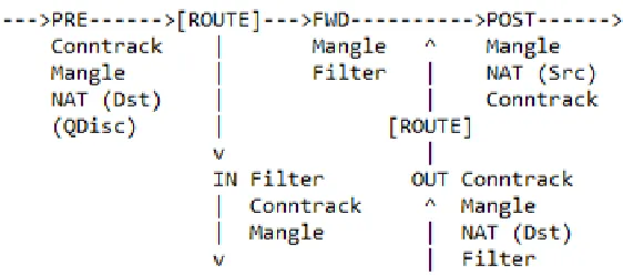
We propose another approach of limiting bandwidth on a particular port as opposed to limiting the traffic for a particular program or process. The process starts with finding out the ports on which a particular application functions which was port 9000 in our case. We mark the packets coming to that port using theNetfilterframework and then pass those packets onto a Linux utility called the traffic controller (tc). The traffic controller is the responsible for throttling the packets coming to it by the means of the hierarchical token bucket algorithm which it utilizes.
the Linux kernel for intercepting and manipulation of network packets. These hooks allow us to capture packets, work on them and insert them back onto the channel via which they are able to reach their original destination. TheNetfilterutility provides us with three tables: NAT, Mangle and Filter. Each table consists of 5 chains essentially Pre-routing, Post-routing, input, output and forward. With the help of those chains, we are able to manipulate the contents of the packets or in our case just mark them with a specific identifier. In our tool, we have used the Mangle table for capturing the
Figure 3.2: The image shows us the path a packet follows through theNetfilterhooks
called as ’filter’. This filter utility function captures those marked packets and applies on it one of the many output algorithms defined for it. In this case we use the hierarchical token bucket algorithm which employs a certain queueing model and manages the throttling for us.
3.5.3 CPU load variation
Variation of the CPU load is one of the core parameters of our model. It gives us a measure of the response of the system when we selectively increase the background noise. This background noise represents the numerous background processes which will be assumed to run while a server instance is running. By selectively varying the total background noise traffic in combination with the other parameters., we obtain a graph of the system response over a range of values.
The CPU load variation is implemented with the help of a set ofdummybots whose function is to jump about in the world and increase the inherent traffic by sending text chat messages to each other. As expected, the more the number ofdummybots we insert into the world, the more is the load on the server and the experiment in general. These bots have been programmed in C# by modifications to thepCampbotcode provided in the OpenSim package. The concept has been explained in Section 4.3.2 of Chapter 4.
3.6
Summary
CHAPTER
4
Metamodelling: Framework and Case Studies
4.1
Introduction
Chapter 4 rests on the analysis of the data obtained by running the simulations based on the experi-mental setup explained in Chapter 3. It begins by providing a brief introduction to the metamodelling approach of approximating system performance. The case studies which have been briefly mentioned in Chapter 3 are elaborated upon further and through detailed analysis of the observations and the methodology described below, we proceed towards building of suitable models. These models, which give us response surfaces are further used for the formulation of optimization problems for cost and time minimization.
4.1.1 Introduction to metamodelling
system dynamics very closely. It is when we use computationally expensive simulation models that it becomes imperative to look for a more practical approach of performance evaluation. Metamodelling, which is an approach of building approximation models is a strategy in which we build a mathematical closed form model of the simulation model. It thus provides an alternative approach through which we can find an approximate mathematical representation of the system performance and can replace the expensive simulation model.
Metamodelling has been studied with regards to computer simulation modeling for over the past three decades even though the term metamodelling was coined in 1987 by Kleijnen [25]. We can find good study resources for this topic in[26]and[17].
Response Surface Modeling (RSM) is the one of the most commonly used methodologies for metamodelling. It was introduced by Box and Wilson in 1951 in their seminal paper[12]on this topic. In their work, followed by their explanation of the concept, they also describe the applications of this concept to chemical processes. RSM has also been discussed in review papers by Hill and Hunter (1966)[21]and Mead and Pike(1975)[27]. The topic has grown over the decades and the techniques have become the topic of entire books as in Box and Draper[13]and Khuri and Cornell[16]. A comprehensive review of the methodology and its applications from 1966 to 1988 has been given in Myerset al. [28].
4.2
The Metamodelling methodology
The Metamodelling methodology is a way of analyzing and deriving a relation between the set of input (CPU and Bandwidth) and output (Time) parameters. We use this method to come up with a mathe-matical model called a Response Surface Model (RSM) to represent this relation and subsequently a response surface which maps together, the input and output values from our experiments.
generally used to approximate the behavior of a system as it can simulate the dynamics of the system in greater detail when compared to an analytical model. Simulation models can be thought of as simple functions that transform input parameters into output values. We however require a closed form response function to correctly understand the behavior of a system. We thus turn to the method of metamodelling which can help us build such a closed form expression and can help us fulfill the purpose of creation of the simulation model by effectively relating the output data of the simulation model to its input parameters. If we have a computational equation representing the input-output relationship of a system as:
Y=f(X1,X2...Xk)
We can realize it as a metamodel, which in its basic form would be represented as:
YG=G(X1,X2...Xk)
Y =YG+ε
whereYGstands for the model andεrepresents both measurement and approximation errors. The most common way to approach metamodelling can be given as follows:
1. Use the experimental design to simulate a number of efficient computer runs and generate output performance data.
2. Choose a metamodel to represent the observed values i.e., the data.
4.2.1 Design of the experiment
An experiment design consists of constructing the experiment though a series of detailed trails. There are a number of ways of doing this, examples of which would be the factorial analysis, orthogonal arrays, the D-optimal method; which is used for the realization of a stochastic process, the select by hand method which is used in neural networks etc. One of the most basic experimental designs and the one which we have used in the analysis is the full factorial analysis. This analysis depends on the number input of factors and the number of levels which we evaluate the input factors at. In our case, the CPU load and bandwidth allocation represent the two factors and we evaluate them at four levels each.
4.2.2 Choosing an appropriate model
The next step is the choice of an appropriate model for approximation of the mathematical and functional relationship between the inputs and outputs. The most commonly used models are response surfaces, neural networks, inductive learning models etc. We are going to use the response surface modeling approach which can be described using polynomial equations of the first order, first order with interactions between its parameters and so on. The standard mathematical polynomial model for a response surface can be written down as:
M(X) =β0+
k X
i=1
βiXi+ k X
i=1
βiXi2+....+ k X
i=1
k X
j=1
βi jXiXj+... (4.1)
This model is based on the observed data and is an empirical model.
We can further derive first and second order models with interactions from the general form given above. The equation of the form first order with interactions would be:
ML(X) =β0+β1X1+β2X2+β3X1X2 (4.2)
X1stands for the number of bots, X2 for the bandwidth while theβs represent constants to be
determined.
Further, we can also define the second order equation for forming a model as:
MN L(X) =β0+β1X1+β2X2+β3X21+β4X22+β5X1X2 (4.3)
These equations are used in the following sections to analyze the observations and to derive response surfaces from them. Further reading material on the topic can be found in [30].
4.2.3 Fitting the model
The conclusive step is to fit the data to the model to approximate the input-output relationship. The fitting method varies according to the choice of the model to be built. (Here we try to build a Response Surface Model.) The usual steps employed by the RSM involve first/second order polynomial equations with factor interactions and least square regression analysis. Other models like neural networks use back-propagation to fit the data.
4.3
Problem Formulation
4.3.1 Problem Statement
The problem can be described as representing the data obtained from the experiments inside the OpenSimulator world as a response surface (as described earlier) and to derive explicit relationships between the input and the output factors. Finally, we need to derive a relationship between the amount of CPU and bandwidth allocation and a proposed cost function.
4.3.2 Inputs
The inputs as discussed earlier are the variation of the allocated bandwidth and the CPU load. Read-ings are taken for these two factors at four levels each. The bandwidth is assigned in magnitudes of 16, 32, 64 and 128 kbps and the CPU load is varied in the form of bots from 20 bots to 80 bots in increments of 20 units. The stress on the server due to the introduction of these bots represents the overall load and the server performance is seen to decrease as we increase thesedummy jumping bots.
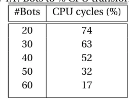
Due to unfortunate circumstances, CPU limiting tools likecpulimithave been proven incompati-ble with our OpenSim platform so we have had to adhere to alternative methodologies for controlling the available CPU for serving the virtual world needs. The CPU load variation is achieved with the introduction of these additionaldummybots as mentioned above, whose function is to jump around the world and broadcast random text messages. Varying the number of these bots instantiated at a particular time gives us a variance in the CPU load. Table 4.1 shows the mapping between the amount of dummy bots and the available CPU cycles dedicated to our server. The transformation function between the number of bots and the allocated CPU cycles is shown below:
λ=α+β∗Bot s (4.4)
Here,λstands for the percentage of available free CPU cycles andαandβare constants. Experi-mental values for these constants in our case turned out to beα=105.6 andβ=−1.45.
Table 4.1: Bots to % CPU transformation #Bots CPU cycles (%)
20 74
30 63
40 52
50 32
4.3.3 Outputs
The outputs of the experimental simulations are readings which represent the amount of time needed for completion of each run. The variation of the input factors has an effect on the time for traversal and we note this effect for gauging the pattern of the response of the server to our input sequences. The measured time readings are observed to range from around 180 sec to 380 sec for the input values provided. The observations have been noted and described in section 4.4 for two different cases, one in which the communication between the bots is assumed to proceed using textual instant messages and another where they are to communicate using something similar to voice communication.
4.4
Case Studies
The framework containing the maze is completely based inside the virtual worldOpenSimulator. As described earlier, there are two bots which form the subject of the experiment. One bot who is responsible for guiding i.e. giving directions to another bot and the other one who is responsible for interpreting those instructions and reacting appropriately. These directions are sent through the means of instant messages from theguide botto the bot inside the maze whom we may call as the lost bot. These messages are to be interpreted correctly by thelost botand the trial should culminate into a successful completion of the maze. The time for completion for each trial is measured from the point at which thelost botteleports to the start of the maze till the finishing point of the maze while successfully interpreting and correctly executing the transmitted instructions. As mentioned in the factorial analysis earlier, we have a number of levels which we use for obtaining the observations. We vary the CPU load and also the allocated bandwidth of the server and observe the effect of the combinational variation has on the output in each scenario.
4.4.1 Case Study 1: The maze with textual message traffic
This case study describes the section of the experiment in which we conduct the experiment with the medium of information exchange being only textual instant messages. As mentioned above, the chat messages exchanged by the bots contain instructions for execution of specific actions. These actions include moving from one location to another on the positional grid of the virtual world by walking to that location, using teleportation to arrive at a certain location on the map i.e., without walking to that spot. (This particular instruction is used at the start of the traversal when we want to align thelost botto the start of the maze.), instructions for correct receipt of an instruction and also for completion of a particular one. Each message of instruction, as mentioned above, is followed by an acknowledgement message which represents successful completion of that particular individual activity i.e. of going from one location to another. An example of a chat message would beGo 156 128. The two numbers following the wordGorepresent the location of the destination point with respect to the X and Y axis of the virtual world. The third axis which is the height of the bot above the ground is assumed to remain the same and hence this piece of information is not transmitted in the instant message.
4.4.1.1 Observations
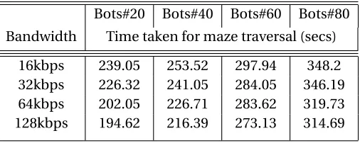
The observations from the experiment for this scenario have been shown in Table 4.2. We take an average of 15 readings per combination of CPU and the allocated bandwidth for determination of each sample trial result. The observations for the above case as mentioned above are obtained by running the simulations of maze traversal with the medium of exchange being only textual instant messages. The observed values, which represent the total time for completion of a single maze traversal, depict an increasing trend as we increase the number of bots i.e., decrease the amount of assigned CPU cycles and show a decrease in magnitude as we increase the amount of allotted bandwidth.
4.4.1.2 Choosing and fitting the metamodel
Table 4.2: Case 1: Chat Message Commands Bots#20 Bots#40 Bots#60 Bots#80 Bandwidth Time taken for maze traversal (secs)
16kbps 239.05 253.52 297.94 348.2 32kbps 226.32 241.05 284.05 346.19 64kbps 202.05 226.71 283.62 319.73 128kbps 194.62 216.39 273.13 314.69
The evaluation of the first order model described in Eq. (4.2) gives us the following resulting equation:
M1L(X) =189.22−0.37X1+1.9X2+0.002X1X2 (4.5)
The analysis of variance (ANOVA) evaluation of the above model, Eq. (4.5) gives us an R-square value of 0.9529. The closer the value of R-square to 1, the better is the model.
We further proceed towards the evaluation of the second order model shown in Eq. (4.3).The new model results in a much higher R-Square value of 0.9854.We thus choose the second model which shows a much better fit, for our RSM. By pluggingβ0=238.525,β1=0.106,β2=−0.949,β3=
0.018,β4=0.004 andβ5=0.002, we can obtain the final equation for our experiment as follows (see
Figure 4.3).
M1N L(X) =238.525+0.106X1−0.949X2+0.018X12+0.004X22+0.002X1X2 (4.6)
4.4.2 Case Study 2: The maze with voice communication traffic
10
20 30
40
50 60
70 80
0 20 40 60 80 100 120 200 250 300 350 400
Bots Response surface
Bandwidth (kbps)
Time (sec)
10 20
30 40
50 60
70 80
0 50 100 150 150 200 250 300 350 400
Bots Response Surface
Bandwidth (kbps)
Time (sec)
Table 4.3: Case 2: Using voice command simulation Bots#20 Bots#40 Bots#60 Bots#80 Bandwidth Time taken for maze traversal (secs)
16kbps 221.28 274.95 358 377.55 32kbps 220.44 262.85 341.69 363.11 64kbps 215.4 259.19 318.07 342 128kbps 208.15 246.30 285.83 313.96
instant message transferred between them. These files occupy extra bandwidth in addition to the occupation of the channel by the textual messages. Since it was tedious to actually transmit voice, and interpret the sent conversational clip inside the virtual world, we have preferred to use the file transfer scheme.
4.4.2.1 Observations
The observations for this scenario have been given in Table 4.3. These readings are also obtained by averaging about 15 readings per sample. The information transmitted in this case constitutes both textual messages and file transfer. The textual messages account for the actual instructions and the file transmission adds to the bandwidth occupancy of the transfer channel. The observed values, which represent the total time for completion of a single maze traversal, depict an increasing trend as we increase the number of bots, i.e., decrease the amount of allocated CPU cycles and show a decrease in magnitude as we increase the amount of allocated bandwidth.
4.4.2.2 Choosing and fitting the metamodel
Figure 4.4):
M2L(X) =169.69+2.8X1+0.04X2−0.009X1X2 (4.7)
Upon evaluating the second order model as represented in equation (4.3), we find that this model has a much better fit with an R-square value of 0.9776. Thus evaluating the model further, we come up with values for our factors,β0=149.314,β1=4.154,β2=−0.225,β3=−0.013,β4=0.002 and
β5=−0.009. Thus the resulting surface for Case 2 can be obtained as shown in Figure 4.5.
M2N L(X) =149.314+4.154X1−0.225X2−0.013X12
+0.002X22+0.009X1X2 (4.8)
ANOVA analysis of the observations shows us a 3% dependence on bandwidth, 32% dependence on the CPU, 1% variations due to interaction and 64% unexplained variation. Focussing on the dependence of the performance on CPU and bandwidth, we still see a major inclination of the server towards allocation of the CPU cycles as compared to the bandwidth.
4.5
Optimum Allocation of Resources
10
20 30
40
50 60
70 80
0 20 40 60 80 100 120 100 150 200 250 300 350 400 450 500
Bots Response surface
Bandwidth (kbps)
Time (sec)
10
20 30
40
50 60
70 80
0 20 40 60 80 100 120 150 200 250 300 350 400
Bots Response surface
Bandwidth (kbps)
Time (sec)
4.5.1 Cost Functions
In this section, we describe our cost functions. The CPU allocation and bandwidth (the two input factors) are used for deriving the cost function. The cost for the bandwidth could be derived with the help of market values for Internet services. Here is the proposed form:
Pb w=γ+δ∗l o g10(φb w) (4.9)
wherePb wis the cost for the allocated bandwidth,φb w represents the input bandwidth in kbps andγ andδare constants whose values were found by fitting the above equation to the data obtained from an internet service provider in our area as,γ=−27.944 andδ=11.402. Alternatively, we could use a linear pricing model which can be shown as:
Pb w=φb w∗pb w (4.10)
where,pb w represents the pricing parameter for bandwidth allocation.
Correspondingly, we propose a cost function for the CPU allocation. The cost function can be written down as:
PC PU=φC PU∗pC PU (4.11)
wherePC PU is the total cost for the CPU,φC PU is the allocation of CPU in cycles andpC PU is the pricing parameter for CPU.
The total costPTot a l is thus:
4.5.2 Optimization Problems
The optimization problems can be stated as follows.
min
φC PU,φb w
Completion Time(φC PU,φb w) (4.13)
Subject toPTot a l <=M,
wherePTot a l is the total cost and M is the monetary budget. Here, we aim to minimize the time needed for completion of the maze as a function of the CPU load and the bandwidth while we are given a certain monetary budget and completion time could be any any of the response surface proposed in Section 4.4
The second problem involves minimizing the cost for running the server given that the time for completion of the maze is less than a given time threshold.
min
φC PU,φb w
Cost(φC PU,φb w)
Subject toCompletion Time<=Tt hr e s hol d (4.14)
whereTT hr e s hol dis the maximum possible time for completion.
4.6
Performance Evaluation
In Table 4.4, we solve the optimization problem shown in Eq. 4.13 where the cost function is the linear one shown in Eq. 4.10 and Eq. 4.11. The pricing parameters arepC PU=1000 CPU pricing units and pb w=5 bandwidth pricing units. The results show that with a higher budget, we can have a higher allocation of CPU/BW that leads to superior performance.
Table 4.4: Results for time minimization
Budget ($) Bandwidth (kbps) CPU cycles (%) Time (secs)
10 1 0.5 358
150 4 12 341.69
350 19 25 283
500 29.8 35 263
800 51 54 229
1000 65 67 211
1500 101 99 184
Table 4.5: Results for cost minimization
Time Budget (sec) Bandwidth (kbps) CPU cycles (%) Cost ($)
185 99.55 97.25 1470
220 58.31 60.47 896
250 37.5 41.9 607
280 20.88 27.9 375.4
310 6.6 14.35 176.5
335 1 2.36 28.7
metric (i.e., time completion) is relaxed the cost decreases but at the same time the resource allocation decreases as well.
4.7
Summary
CHAPTER
5
Conclusion
We conclude the thesis with a brief summary of the work conducted by us on the topic and some related future work.
5.1
Summary
Virtual worlds as we know are growing at a tremendous pace and so are the computing requirements of such environments. It is thus imperative that we be proactive in optimizing the networking assets and processing power at hand while making sure that we do not compromise on the social networking aspect of these work spaces. A small change in the technical parameters can change the user experience. Analysis of the social aspect of this problem adds a new facet to the analysis of the performance of this framework. The kind of objects the user interacts with inside the world and the method and quality of their depiction can dictate the way a DE student understands a lecture taught remotely.
world and that we needed to model the performance characteristics according to the preferences of the subject i.e. the user. We needed to analyze such a world in order to create a framework keeping the user’s preferences in mind. Thus, analysis of the the perceptions of the users was a step necessary for modeling the performance parameters and also the framework. The proposed framework provided us with a base to model these performance characteristics and modulation of these characteristics enabled us to study these environments at a much greater depth.
We realized that high bandwidth networks and processors really play an important role in defining and controlling the quality of this term:virtual presence. It is obvious that providing the best network-ing qualities and good processors can give us the best performance. But in the advent of this grownetwork-ing demand for resources, it is necessary we utilize them in an optimum way and that being judicious holds the key. We thus have gone ahead with our design of the framework to obtain an understanding of the performance demands of these environments.
5.2
Future work
In this section, we propose a number of areas for future work in the topic of performance analysis of VCEs using networking capabilities.
5.2.1 Conducting the experiments with human subjects
The framework which was originally designed with the engineering of these experiments with human subjects in SecondLife (in the place of bots). Conducting the trials with human subjects could give us a new insight in this domain.
5.2.2 Resource optimization with the marketing point of view
Detailed analysis of the cost and time optimization with regards to the performance metric of VCEs could be carried out with respect to the marketing aspect of the area.
5.2.3 Analysis of the VCE with actual voice transmissions
REFERENCES
[1] Croquet project. http://www.opencroquet.org/.
[2] Cyberlandia. http://www.cyberlandia.net/.
[3] Kaneva. http://www.kaneva.com.
[4] Open software foundation. wiki: http://en.academic.ru/dic.nsf/enwiki/126389.
[5] Open source metaverse project. http://metaverse.sourceforge.net/.
[6] Pseudospace. http://www.pseudospace.net/.
[7] Quest atlantis. http://atlantis.crlt.indiana.edu/.
[8] Sciencesim. http://sciencesim.com/wiki/doku.php.
[9] SecondLife. http://secondlife.com/.
[10] Reina Y. Arakji and Karl R. Lang. Avatar Business Value Analysis: A Method for the Evaluation of
Business Value Creation in Virtual Commerce. Journal of Economic Commerce Research, 2008.
[11] Jared E. Bendis. Developing educational virtual worlds with game engines. InSIGGRAPH ’07: ACM SIGGRAPH 2007 educators program, page 26, New York, NY, USA, 2007. ACM.
[12] G. E. P. Box and K. B. Wilson. On the experimental attainment of optimum conditions.Journal of the Royal Statistical Society. Series B (Methodological), 13(1):1–45, 1951.
[13] George E P Box and Norman R Draper. Empirical model-building and response surface. John Wiley & Sons, Inc., New York, NY, USA, 1986.
Moham-FDG ’09: Proceedings of the 4th International Conference on Foundations of Digital Games, pages 232–239, New York, NY, USA, 2009. ACM.
[15] Luis Diego Briceño, Howard Jay Siegel, Anthony A. Maciejewski, Ye Hong, Brad Lock,
Moham-mad Nayeem Teli, Fadi Wedyan, Charles Panaccione, and Chen Zhang. Resource allocation in a client/server hybrid network for virtual world environments.
[16] J. A. Cornell.Response surfaces: designs and analyses. Marcel Dekker, Inc., New York, NY, USA, 1987.
[17] M. Isabel Reis dos Santos and Acácio M.O. Porta Nova. Statistical fitting and validation of
non-linear simulation metamodels: A case study.European Journal of Operational Research, 171(1):53 – 63, 2006.
[18] Marius A. Eriksen. Trickle: a userland bandwidth shaper for unix-like systems. InATEC ’05: Proceedings of the annual conference on USENIX Annual Technical Conference, pages 43–43, Berkeley, CA, USA, 2005. USENIX Association.
[19] S. de Freitas, G. Rebolledo-Mendez, F. Liarokapis, G. Magoulas, and A. Poulovassilis. Developing
an evaluation methodology for immersive learning experiences in a virtual world. InVS-GAMES ’09: Proceedings of the 2009 Conference in Games and Virtual Worlds for Serious Applications, pages 43–50, Washington, DC, USA, 2009. IEEE Computer Society.
[20] M. Gerhard, David J. Moore, and Dave J. Hobbs. Continuous presence in collaborative virtual
environments: Towards a hybrid avatar-agent model for user representation. InIVA ’01: Proceed-ings of the Third International Workshop on Intelligent Virtual Agents, pages 137–155, London, UK, 2001. Springer-Verlag.
[21] William J. Hill and William G. Hunter. A review of response surface methodology: A literature
survey.Technometrics, 8(4):571–590, 1966.
[22] Clyde W. Holsapple and Jiming Wu. User acceptance of virtual worlds: the hedonic framework.
[23] Jie Hui. Abstract hui, jie. qos provisioning in wi-fi networks: Capacity modeling and resource,
2005.
[24] Philippe Kerremans. Metaverse business launches event analysis tool for virtual worlds.
[25] Jack P C Kleijnen.Statistical tools for simulation practitioners. Marcel Dekker, Inc., New York, NY, USA, 1986.
[26] Jack P. C. Kleijnen. Verification and validation of simulation models. European Journal of Operational Research, 82(1):145 – 162, 1995.
[27] R. Mead and D. J. Pike. A biometrics invited paper. a review of response surface methodology
from a biometric viewpoint.Biometrics, 31(4):803–851, 1975.
[28] Raymond H. Myers, André I. Khuri, and Jr. Carter, Walter H. Response surface methodology:
1966-1988.Technometrics, 31(2):137–157, 1989.
[29] Robert G. Sargent. Research issues in metamodeling. InWSC ’91: Proceedings of the 23rd conference on Winter simulation, pages 888–893, Washington, DC, USA, 1991. IEEE Computer Society.
[30] Timothy W. Simpson, J. D. Poplinski, P. N. Koch, and J. K. Allen. Metamodels for computer-based
engineering design: Survey and recommendations.Eng. Comput. (Lond.), 17(2):129–150, 2001.
[31] Xavier Vilajosana, Daniel Lázaro, Angel A. Juan, and Leandro Navarro. Towards decentralized
APPENDIX
A
A.1
Configuring the OpenSim core server
We start with the basic installation guidelines for configuring the server. The steps are given below. 1. The OpenSim installation file can be downloaded from[put the reference here]. We extract the file on our machine and run the runPrebuild.bat file in the top directory. 2. We next open the resulting .sln file with visual studio and build it in place or run the compile.bat file. 3. Running nant in the same subdirectory will build the file. 4. We start the server with the command - ReplaceSYSTEMIPwith the ip address of your server.
Post-Installation.
1. Inside bin directory, we make a copy of the OpenSim.ini.example file as OpenSim.ini Making walls opaque
Open the fileOpenSim.ini
Regions.ini or default.xml located inside the directory/bin/Regions Changes: change the internal IP address to 0.0.0.0
confirm that SystemIp is the IP address of the system.
3. Flattening the terrain
change region<Region_Name> terrain fill 21
4. Loading and saving the terrain load oar<Terrain_Name> save oar<Terrain_Name>
5. Disable authentication checks
Inside OpenSim.ini, modify value of authentication to: authentication=false
6. Changing the gravity of the region to correct the posture of bot and avoid bent legs. Inside OpenSim.ini, changeav_capsule_standup_tensor_linux=1700000from its old value - 500000.
7. Changing the landing point. To make sure that the inception point of all bots does not coincide with the maze.
(a) In each region, go to the place where you would like yourself and others to arrive at.
(b) From your viewer go toAbout Land(by clicking on the Region name at the top of your viewer screen in the middle of the menu bar).
(c) click on theOptionstab.
(d) set theTeleport RoutingtoLanding Point.
A.2
Configuring the OpenSim voice server
Voice capability can be installed on the OpenSim server through the installation of a module called FreeSwitch.
The FreeSwitch module is available externally for download and is available for 32bit systems. The installation steps are as follows.
1. Install FreeSwitch by executing the FreeSwitch binary downloaded.
2. Open /FreeSwitch/conf/autoload _configs/modules.conf.xml.
3. Uncomment<load module="mod_siren"/>.
4. Uncomment<load module="mod_xml_curl">.
5. Save the filemodules.conf.xml.
6. Open /FreeSwitch/conf/autoload_configs/xml _curl.conf.xml.
7. Change the configuration to matchhttp://opensimulator.org/wiki/FreeSwitch _Moduleand save it.
8. OpenFreeSwitch/conf/vars.xml.
9. Add a new codec toglobal_codec_prefs:G722132000h, save the file.
10. Open and setupOpenSim.ini.
11. Search for the[FreeSwitch]section and makeenabled=true.
12. Make sure all instances ofip.address.of.freeswitch.serverare modified to equal your server’s ip_ address, save the file.
15. Start the client and go to user preferences.
16. Uncheck the enable voice chat option.
17. Go to estate options and make sure that the allow voice chat option is checked.
18. Go toAbout Land, click on themediatab and check theUse a private spatial channeloption.
19. Go again touser preferences,voice chattab and check the EnableVoice chat option.
20. Voice chat should be enabled inside OpenSim now and you can use it by pressing the talk button on the bottom right of your client.
A.3
Scripting code - Opensim
The OpenSimulator environment uses its own internal scripting language for programming objects inside the world. For eg. If your avatar comes up against a door inside the world and you want to open the door to entire or exit the structure, clicking on the door can activate a script which would open the door for you. Such scripts are embedded in virtual objects inside these environments.
A.3.1 LSL example code snippets
A.3.1.1 Distance Monitor
// Distance calculator. vector lPos = <135,114,22.6>;
//Modify acc to start position <133.29,114.081,20.906> float dist_traveled = 0;
integer listen_handle; default
{
state_entry() {
listen_handle = llListen(12,"","",""); }
//Listen for distance broadcasts
listen(integer channel, string name, key id, string message) {
if(message != "reset distance") {
vector pos = (vector)message; float xDist = pos.x - lPos.x; float yDist = pos.y - lPos.y;
dist_traveled += llSqrt(xDist*xDist + yDist*yDist);
//Display the distance traveled
llSay(0,"Distance traveled: "+(string)dist_traveled); lPos = pos;
if(pos.z == 1 && xDist==0 && yDist==0) {
dist_traveled = 0; }
else if(pos.z == 1 && xDist!=0) {
//llShout(0,"Distance traveled: "+(string)dist_traveled); }
}
if(message == "reset distance") {
dist_traveled = 0; lPos = <135,114,22.6>; }
}
// If someone clicks on the object, display the last noted distance. touch_start(integer total_number)
{
// Display the distance.
A.3.2 Bandwidth control code
Bandwidth limitation was done by throttling the packet arrival and departure rate on a certain port on the system. The packets were marked using the Netfilter module and then their rate of flow was restricted using the code snippet displayed in Figure A.2.
#Create the root handle for qdisc
sudo /sbin/tc qdisc add dev eth0 root handle 1:0 htb
#Add a class with the rate
sudo /sbin/tc class add dev eth0 parent 1:0 classid 1:1 htb rate 128kbit #Add a filter with the class id of the above class
#sudo /sbin/tc filter add dev eth0 protocol ip handle 6 fw classid 1:1
sudo /sbin/tc filter add dev eth0 protocol ip handle 7 fw classid 1:1
#Display the created filter sudo tc -s filter show dev eth0
#Display the created class sudo tc -s class show dev eth0