HIGHLIGHTED ARTICLE
| INVESTIGATION
A General Approximation for the Dynamics of
Quantitative Traits
Katarína Bod’ová,1Gasper Tkaˇ cik, and Nicholas H. Bartonˇ Institute of Science and Technology Austria (IST Austria), Klosterneuburg A-3400, Austria
ABSTRACTSelection, mutation, and random drift affect the dynamics of allele frequencies and consequently of quantitative traits. While the macroscopic dynamics of quantitative traits can be measured, the underlying allele frequencies are typically unobserved. Can we understand how the macroscopic observables evolve without following these microscopic processes? This problem has been studied previously by analogy with statistical mechanics: the allele frequency distribution at each time point is approximated by the stationary form, which maximizes entropy. We explore the limitations of this method when mutation is small (4Nm,1) so that populations are typically close tofixation, and we extend the theory in this regime to account for changes in mutation strength. We consider a single diallelic locus either under directional selection or with overdominance and then generalize to multiple unlinked biallelic loci with unequal effects. Wefind that the maximum-entropy approximation is remarkably accurate, even when mutation and selection change rapidly.
KEYWORDSquantitative genetics; maximum entropy; diffusion approximation, quasi-stationarity
M
OST traits of interest have a complex genetic basis depending on very many loci. Quantitative genetics gives a sophisticated statistical description of the components of trait variance that can predict the immediate change due to selection. The present abundance of genetic markers allows us to find some of the loci that affect traits, but such QTL typically account for only a small fraction of the genetic variance (Hill and Kirkpatrick 2010; Yanget al.2010). While we may be able to predict breeding values and estimate the distribution of effects, it does not seem possible—even in principle—to iden-tify the individual alleles responsible for the bulk of heritable variance. Thus, we cannot hope to predict the evolution of quantitative traits by using a direct population genetics ap-proach based on the frequencies of each individual allele.Here we develop a general method that allows us to closely approximate the evolution of quantitative traits knowing only the distribution of allelic effects and mutation rates but without requiring knowledge of individual allele frequencies. This can be seen as an extension of the classical infinitesimal
model to include arbitrary gene interactions and the effects of selection, mutation, and drift on the genetic variance. It also can be viewed as a generalized version of the quasi-steady-state assumption (QSSA) that is often made in dynamical reaction systems (Segel and Slemrod 1989; Goeke and Walcher 2013) to noisy systems described by partial differ-ential equations (PDEs), where the dynamics are approxi-mated using a quasi-stationary distribution assumption (QSDA); here we use the maximum-entropy (MaxEnt) prin-ciple to define that distribution.
In physics, the MaxEnt principle has a long history, starting with the seminal work of Jaynes (1957), who interpreted the Boltzmann distribution of statistical physics as the most ran-dom distribution subject to a constraint onfixed average en-ergy. In the recent decade, there has been a resurgence of interest in MaxEnt, especially when applied to biophysics problems ranging from the statistics of neural spiking (Schneidmanet al.2006; Tkaˇciket al.2014), birdflocking (Bialeket al.2012), protein structure (Weigtet al.2009), and immunology (Moraet al.2010). These approaches have been generalized to describe temporal dynamics of high-dimensional systems, known collectively asmaximum-caliberordynamical/ kinetic maximum-entropy models (Presséet al.2013), where the entropy of distribution over temporal paths is maxi-mized given constraints on dynamical variables. Surprisingly,
Copyright © 2016 by the Genetics Society of America doi: 10.1534/genetics.115.184127
Manuscript received October 28, 2015; accepted for publication February 9, 2016; published Early Online February 16, 2016.
Supplemental material is available online at www.genetics.org/lookup/suppl/ doi:10.1534/genetics.115.184127/-/DC1.
1Corresponding author: Institute of Science and Technology Austria (IST Austria), Am
however, MaxEnt distributions have not been used widely as a variational ansatz for cases discussed in this work, where the evolution equation for the distribution might be knowna priori, e.g., as is the case with the diffusion approximation in popula-tion genetics. In such a case, the approach differs from the maximum-caliber methods because it involves a combination of a static MaxEnt ansatz for the stationary microscopic distri-bution with a quasi-stationary assumption in the diffusion/ Fokker-Planck equation, which together extend the static MaxEnt inference to a dynamical approximation.
Prügel-Bennett and Shapiro (1997) and Rattray and Shapiro (2001) introduced the MaxEnt approximation to the dynamics of polygenic systems, predicting the cumulants of the trait dis-tribution under mutation, selection, and drift; their main moti-vation was to understand evolutionary algorithms rather than natural populations. The same method was described indepen-dently in physics (Plastinoet al.1997) and used to approximate cosmic-rayfluxes (Hick and Stevens 1987).
However, neither of the two applications of MaxEnt was taken up in their respectivefields. Barton and de Vladar (2009) modified Prügel-Bennet, Rattray, and Shapiro’s method so that it could be justified from population genetics principles. With this modification, it gives the stationary distribution exactly and is accurate in the limit of slowly changing conditions. Numer-ical calculations showed that it is remarkably accurate, even when selection or mutation changes abruptly. However, the method is fully valid only when mutation is stronger than drift (4Nm.1), so populations are almost neverfixed for one or other allele. Yet, in nature, mutation is typically weaker than drift, so most sites arefixed; in this case, Barton and de Vladar’s approximation applies only in cases where mutation or popu-lation size does not change with time.
We begin by summarizing the stationary MaxEnt approxi-mation and its extension to nonstationary problems. We then extend the MaxEnt approximation so that it applies over the full range of mutation rates and test the accuracy of this approxi-mation for directional selection and for balancing selection that favors heterozygotes. This extension is a combination of the continuous approach of Barton and de Vladar (2009) and a special treatment of the dynamics at the boundaries. A similar approach, where the boundaries have to be treated differently, has been used in the semidiscrete, semicontinuous methods studied in reaction-diffusion systems (Flegg et al. 2011; Robinsonet al.2014) and also in travelingfitness waves, where thefluctuations can be introduced to the model using a cutoff function (Tsimringet al.1996; Hallatschek 2011). We initially consider the distribution of allele frequencies at a single locus and then extend consideration to multiple loci with a distribu-tion of effects. Throughout, we assume that recombinadistribu-tion is fast relative to other processes so that the population is in link-age equilibrium and can be described by its allele frequencies.
Dynamics of Allele Frequencies
The dynamics of allele frequenciesp¼ ðp1;. . .;pLÞ(for bial-lelic loci) can be described by a diffusion process using a
deterministic forward Kolmogorov equation (i.e., the Fokker-Planck or diffusion equation). The evolution of the joint prob-ability densitycðp;tÞof allele frequencies satisfies
@c
@t ¼ 2 XL
i¼1
@ @pi
½MiðpiÞc þ1 2
XL
i¼1
@2
@p2i ½ViðpiÞc (1)
where the number of loci that contribute to the trait isL. The second term of (1) equalsViðpiÞ ¼piqi=2Nand cap-tures stochasticity of the allele frequencies arising from ran-dom sampling, i.e., the random drift. While in the case of linkage disequilibrium this term would contain a double sum-mation, reflecting correlations between loci, the off-diagonal terms vanish at linkage equilibrium. (The factors of 2 in the brackets of (1) arise because we assume a diploid population ofNindividuals; the corresponding haploid model would be the same, apart from these factors.)
The first term of (1) captures deterministic changes of allele frequencies. We consider
MiðpiÞ ¼ ðbgiþhhiÞpiqi
12 2hhi bgiþhhipi
þmqi2npi
(2)
wherebis the strength of directional selection,hdenotes a higher-order correction that captures dominance,mandnare the forward and backward mutation rates, andgiandhiare the additive effects of theith locus on the traits under selec-tion.MiðpiÞcan be written in a potential form
MiðpiÞ ¼piqi 2
@ðaAÞ
@pi
where the potentialaA, obtained by inverting this relation-ship, reflects effects of selection and mutation:
aA¼ X j
ajAj¼logWþmUþnV
¼bzþhHþ2mX
L
i¼1
logpiþ2n
XL
i¼1
logqi
(3)
with quantitiesz,U,V, andHdefined as
z¼X
L
i¼1
giðpi2qiÞ ; H¼
XL
i¼1
2hipiqi (4)
U¼X
L
i¼1
2 logpi; V¼
XL
i¼1
2 logqi (5)
whereqi¼12pi, andgiandhiare the effects of loci on the traitszandH, respectively.
selection coefficients and Aw various selected traits. In the case of dominance, the terms associated with selection are logW¼bzþhH¼awAw, where aw¼ ðb;hÞ and
Aw¼ ðz;HÞ. Here we assume a weak selectionb1 such that logWlogW.
The deterministic effects on allele frequency can be sum-marized into a vector of coefficientsaand a vector of com-plementary quantitiesA. We study directional selection and dominance with nonsymmetrical mutation and defineaand
Aas
a¼ ðb;h;m;nÞ; A¼ ðz;H;U;VÞ (6)
In the sections that follow, we show that A and a can be understood as constraints and corresponding Lagrange mul-tipliers, respectively, of a particular variational problem.
Forh¼0 andm¼n, this represents the simplest scenario of directional selection with symmetrical mutation. Directional selection of strengthbacts on a traitz, assumed to be additive, while selection of strengthhacts on heterozygosityH. In this work, we consider unequal effects gi on the trait but equal effectshi¼1 onH. This can be easily extended to distribution of effectshi. A wide variety of other models can be treated in the same way. For example, de Vladar and Barton (2011) stud-ied stabilizing selection on an additive trait.
This diffusion process is known to be an accurate contin-uous-time approximation to a wide range of specific popula-tion genetics models (Kimura 1955a; Ewens 2012); moreover, it corresponds directly to the coalescent process that describes the ancestry of samples taken from the popu-lation (Wakeley 2008). In order to represent the popupopu-lation in terms of allele frequencies, we must assume that linkage disequilibria are negligible, which will be accurate if recom-bination is sufficiently fast. For simplicity, we also assume two alleles per locus.
The stationary distribution of (1) has the form (Wright 1931; Kimura 1955a)
cðpÞ ¼1
ℤexpð2NaAÞ
YL
i¼1 ðpiqiÞ21
¼1
ℤW
2NYL
i¼1
p4Ni m21q4Ni n21
(7)
whereℤis a normalization constant, also called apartition function. This distribution falls to zero at the boundaries (p = 0, 1) provided that 4Nm.1 and 4Nn.1. However, when mutation rates fall below this threshold, the distribution de-velops singularities at boundaries (if 4Nmor 4Nnis small, the singularity occurs at p = 0 or p = 1, respectively), even though the density function is still integrable.
MaxEnt in Equilibrium Quantitative Genetics
The stationary distribution (7) can be derived from a varia-tional MaxEnt principle. The key assumption is that selection and mutation act only through a set of observable quantities,
which can be arbitrary functions of allele frequencies
A¼ fAiðpÞg; the strength of selection and mutation is given by the corresponding set ofa¼ faig. Together these define the potential functionaA.
We can define an entropy, relative to a reference measure fðpÞ, as
SH½c ¼ 2 Z
½0;1L
cðp;tÞlog
cðp;tÞ fðpÞ
dp (8)
which has a unique maximumcðp;tÞ ¼fðpÞat the reference distribution; the entropy is (minus) the Kullback-Leibler di-vergence from fðpÞ. The key choice is to set the reference distribution as the neutral distribution of allele frequencies in the absence of mutation or selection:
fðpÞ ¼Y
L
i¼1
ðpiqiÞ21 (9)
Note thatfðpÞis not integrable, but it does provide the neu-tral probability distribution given that the allele is notfixed and yields the stationary distribution under mutation, selection, and drift when we maximize SH subject to a normalization constraint and constraints hAi ¼ hAiobs. The latter condition enforces a constraint on the ensemble aver-ages hAðpÞi ¼RAðpÞcðpÞdp. These macroscopic quantities represent information that, in principle, could be observed. We refer tohAðpÞias observables, even though this does not necessarily mean that their values over time are known. The constrained maximization of entropy is solved by a method of Lagrange multipliers; for details, see Appendix A. For the example in (6), the constraints include
1. R½0;1LcðpÞdp¼1–normalization constraint,
2. hzi ¼ hziobswith Lagrange multiplier 2Nb, 3. hHi ¼ hHiobswith Lagrange multiplier 2Nh, 4. hUi ¼Uobswith Lagrange multiplier 2Nm, and 5. hVi ¼Vobswith Lagrange multiplier 2Nn.
The normalization condition sets the total probability of the allele frequency distribution to 1 and introduces the partition functionℤas a constant multiplier in (7).
genetics, A characterizes properties of a quantitative trait whose means can be observed (hAi) and that evolves in re-sponse to the evolutionary forcesa. In statistical physics,A andarepresent conjugate pairs of thermodynamic variables, which can be interpreted as the constraints and Lagrange multipliers in the variational MaxEnt problem, commonly encountered when microscopic states of the system are un-observed but its macroscopic features are known.
Note that there is some flexibility in the choice of the reference distributionfðpÞ, where different choices may lead to the same stationary distribution. For instance, one may take the neutral distribution that involves mutation terms fðpÞ ¼Qkpi4Nm21q4Nn21
i while omitting the constraints on U andV and assuming thatm andnare functions of time. In this way, the reference distribution would be normalizable. Because these approaches are equivalent, one can view the constraints onUandVas conditions that regularize the allele frequency distribution.
Dynamic MaxEnt Approximation
Our aim is to approximate the dynamics of a high-dimensional system by a small number of variables, which include the quantities that determine fitness. We approximate the real distribution of allele frequencies by the stationary distribution obtained by the MaxEnt method with a small number of constraints and use it as an ansatz in the diffusion equation. This leads to effective dynamical forces a* that yield the correct dynamics for the observed quantities. The assumption
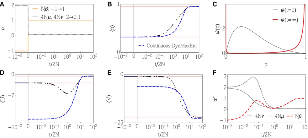
that the population is perturbed only through the forcesais crucial to the success of our approximation. If we could ma-nipulate individual allele frequencies in an arbitrary way, then the long-term evolution would become essentially un-predictable: alleles that are initially rare could increase to cause arbitrary changes as they eventually rose to apprecia-ble frequency (Barton and de Vladar 2009) (Figure 1). The overall strategy of the dynamical MaxEnt (DynMaxEnt) ap-proximation is summarized in Table 1, while the terminology from statistical physics and quantitative genetics is provided in Table 2. Various approximate methods, discussed in our work, are summarized in Table 3.
Wefirst describe the continuous DynMaxEnt method, pro-posed in Barton and de Vladar (2009), which requires a suf-ficient number of mutations in every generation. However, a discrete approximation, also used in Barton and de Vladar (2009) and described in Appendix C, is applicable when the mutation rate is small and selection is limited. The dynamics are then formulated in terms offixed classes of alleles. How-ever, the discrete approximation is not accurate unless the mutation rate is very small, and even then it has a limitation when Nb1 (Appendix C). Similarly, the continuous method fails for 4Nm ,1 (Appendix D). We compare the performance of these methods in Appendix G andfind that while the discrete method applies to a very small mutation rate and the continuous method to a large mutation rate, the intermediate regime is not captured by either of them. This is similar to the result of Mustonen and Lässig (2007, 2008), who studied fitness waves in the problem of fluctuating
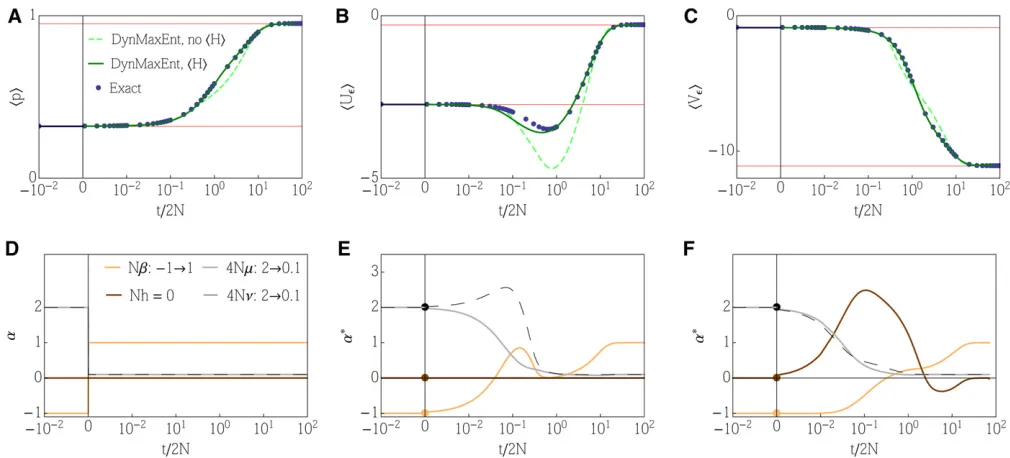
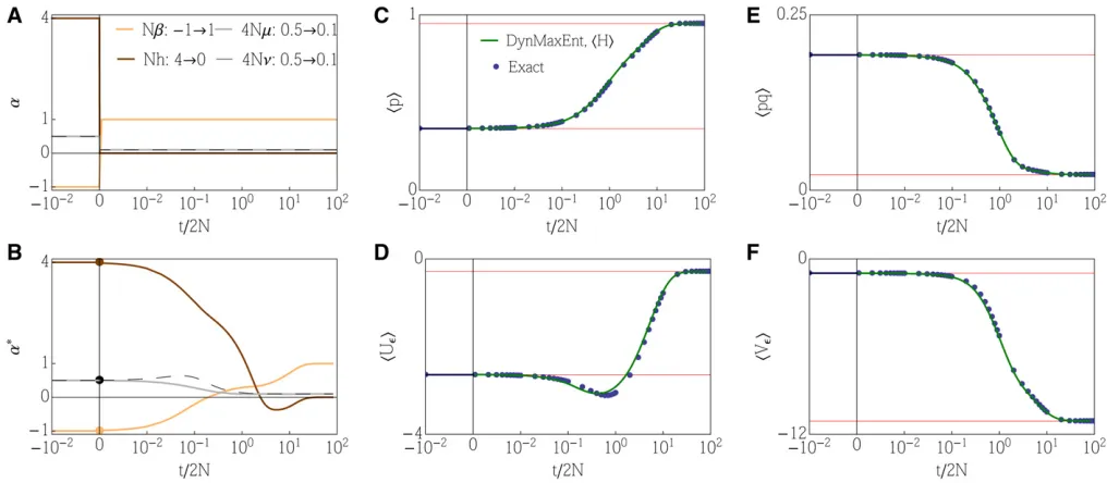
Figure 1 Example 1: details of the general DynMaxEnt method. The response of the observed quantities: (A–C) Observableshpi,hUei, andhVei
selection and introduced a novel approximation that is accu-rate for small selection timescales. Figure 2 in Mustonen and Lässig (2008) also shows an intermediate regime in which neither the diffusion theory nor the novel approximation is accurate. In this work, we present ageneral DynMaxEnt ap-proximation that is applicable in all regimes. This approxima-tion is compared to the numerical soluapproxima-tion of the diffusion equation. Instead of using individual-based simulations, which are computationally demanding, we consider allele frequencies to hold biologically relevant values pk¼k=2N,
for k¼0;. . .;N, and forward iterate an explicit transition matrix, consistent with the diffusion equation. This approach, provided in a Mathematica notebook (Supplemental Material,File S1), is also feasible when a moderate number of loci have different effects on the trait of interest.
Continuous DynMaxEnt approximation
Any set of forcesawill cause the population to evolve to a stationary distributionðf=ℤÞexpð2NaAÞ; this is the distri-bution that maximizes entropy subject to constraints onhAi, the 2Nabeing the Lagrange multipliers. Now suppose that the forces change abruptly, from a0 to a1, and no further information about the system is provided. The expected ob-servableshAiwill evolve toward the new stationary distribu-tion. At any time, there will be a set of forcesa* that would produce the currenthAiif the population were stationary; we expect that thea* will evolve froma0toa1as the population evolves from one stationary state to the other. Thus, we can describe the dynamics either by the change inhAior, equiv-alently, by the change ina*.
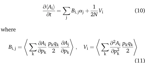
Under the diffusion approximation, the expectations change as
@hAii
@t ¼ X
j
Bi;jajþ 1
2NVi (10)
where
Bi;j¼
* X
k
@Ai
@pk
pkqk
2
@Aj
@pk
+
; Vi¼
* X
k
@2A i
@p2 k
pkqk
2 +
(11)
[Equations 13 and 14 of Barton and de Vladar (2009); note that in their Equation 13 the expectation should be taken over the whole equation, not inside the derivatives as typed].
The expectations that appear on the left-hand side of (10) are not the same as the ones on the right; therefore, the system is not closed. We now introduce the continuous DynMaxEnt approximation, namely, that Bi;j andVi in the dynamically changing system are approximated by the values that they would have at the corresponding stationary state that gener-ates the actualhAi; the stationary distribution coincides with the MaxEnt distribution. If the population were at a station-ary state under the forcesa*, chosen to produce the current expectationshAi, then there would be no change:
@hAii
@t ¼0¼ X
j
B* i;ja*j þ
1 2NV
*
i (12)
where the asterisks denote values at the stationary distribu-tion. The approximation has form ð1=2NÞV*
i 2 P
jB*i;ja*j, which gives Equation 15 of Barton and de Vladar (2009) as
@hAii
@t ¼ X
j
B* i;j
aj2a*j
(13)
It may be more convenient to follow the rates of change ina*, which can be written in terms of the covariance of fluctua-tions in theA. Using matrix notation,
@a*
@t ¼ 1
2NC*21B* ða2a*Þ (14)
where
C*¼CovðAi;AjÞ ¼
@2logℤ
@ai@aj
(15)
with an initial conditiona*(0) =a0anda=a1. The differ-enceja12a0jrepresents the change in evolutionary forces. Because the matricesB* andC* depend only on the effective forcesa*, as shown in Appendix B, the dynamical system for a* is closed. A detailed derivation of the DynMaxEnt method under more general conditions can be found in Appendix E. Intuitively, one may assume quasi-stationarity in (10), provided that the evolutionary forcesachange on a slower timescale than the timescales of selection (1/b), mutation (1/m), and random drift (2N). Then the adiabatic approxi-mation in (14) should be accurate not only for the predicted observables but also for the microscopic distribution. However, we will show that even when the evolutionary forces change
Table 1 Summary of the DynMaxEnt approach in four steps
Step 1 Formulate dynamics, as in (1), for the probability distribution of the state variablescðpÞ.
Step 2 Obtain the stationary distributioncand write it in an exponential (log-linear) formcðpÞ}fðpÞexpð2NaAÞin terms of observableshAiand constant forcesa.
Step 3 RepresentcðpÞas a solution of a variational MaxEnt problem with reference distributionfðpÞ, constraints onhAi, and Lagrange multipliersa(nonunique).
Step 4 Use a quasi-stationarity assumption to approximate the dynamics of observables using the stationary distribution where the coefficientsaare allowed to change over time to match the correct dynamics of observables. This criterion leads to a reduced dynamical system for the effective coefficientsa*.
abruptly,i.e., whenja12a0jis not small, the approximation remains accurate—even though there is no guarantee that the inferred microscopic distribution agrees with the correct one.
The matrixBcan be seen as a generalization of the addi-tive genetic covariance matrix, where the @Ai=@pk corre-sponds to (twice) the marginal effects of the kth allele on Ai. The MaxEnt approximation consists of assuming that this matrix is approximately what one would obtain at equilib-rium with the currenthAi. Thus, (13) is an extension to the ”breeder’s equation”(Lynch and Walsh 1997), which allows for quantitieshAithat can be any function of allele frequencies— not just trait means—and that allows for randomfluctuations, mutational bias, and nonadditive selection.
The DynMaxEnt method can be contrasted with the maximum-caliber method, reviewed in Pressé et al. (2013). DynMaxEnt uses static observables to infer the correct sta-tionary allele frequency distribution but allows the Lagrange multipliers to change over time in accordance with the known diffusion equation, ensuring that the observables are correct at all times. However, the maximum-caliber method uses constraints on temporal characteristics to arrive at a distribution over the allele frequency paths with constant values of Lagrange multipliers. DynMaxEnt is suitable for our problem because it only assumes knowledge of initial and changed evolutionary parameters and no further information on the properties of the allele frequency paths.
General DynMaxEnt approximation
When numbers of mutations are small (i.e., 4Nm , 1 and 4Nn ,1), we face a problem of diverging components in the continuous DynMaxEnt approximation as a result of a U-shaped allele frequency distribution (for simplicity, we will consider a single locus). IfA¼ ðz;H;U;VÞ, this divergence is caused by diagonal elements of matrixBthat correspond toU and V, in particular, B3;3¼ hpq=2 ½@pUðpÞ2i ¼ h2q=pi for 4Nm ,1 and B4;4 ¼ hpq=2 ½@pVðpÞ2i ¼ h2p=qi for 4Nn, 1 (see Appendices B and D for more detail). Therefore, the continuous DynMaxEnt approximation fails completely in a regime of dynamic selection and mutation when 4Nm,1 or 4Nn,1 simply because the right-hand side of the dynamical system (14) is ill defined. The breakdown of the continuous
DynMaxEnt method, when the number of mutations are small (i.e., for small populations), is not a numerical problem but a fundamental limitation of the method itself. However, it can be avoided by considering a modified diffusion problem that does not aim to resolve all details of the allele frequency distribution close to thefixation and loss but instead agrees with the original problem in terms of the probability that the allele frequency is extreme.
We define the boundary layers as½0;eÞandð12e;1for
e1 butfinite. The value of the truncation parametereis discussed later, but typically,e1=N. We then replace the original diffusion equation with solution cðp;tÞ by a new system of PDEs with solution ceðp;tÞ that agrees with the true dynamics in the following properties:
1. The stationary distribution in the bulk is the same for both problems:ceðp;t¼NÞ ¼cðp;t¼NÞ, forp2 ½e;12e. 2. The stationary probabilities of extreme allele frequencies
are the same for both problems:
P½p,e ¼ Ze
0
cðp;t¼NÞdp¼ Ze
0
ceðp;t¼NÞdp
and
P½p.12e ¼ Z1
12e
cðp;t¼NÞdp¼ Z1
12e
ceðp;t¼NÞdp
to the lowest order ine.
3. As the truncation parameter goes to 0, the problem con-verges to the original diffusion equation;i.e., it develops singularities at the boundaries:
lime/0ceðp;tÞ ¼cðp;tÞ:
Replacing the original diffusion equation with a set of coupled diffusion equations in different regions of the state space captures an important characteristic of the problem: the presence of multiple timescales in the allele frequency dy-namics. When the system is perturbed from stationarity by a change in the Lagrange multipliers (selection, mutation, het-erozygosity),e.g., by a dramatic drop in number of mutations, the correct distribution very quickly adjusts to the form p4Nm21q4Nn21 at the boundaries. Only then does the mass in the interior slowly transfer to the vicinity of thefixed states to converge to the new stationary distribution. This results in a very fast dynamics ofhUiandhViand a considerably slower dynamics of the trait mean and the mean heterozygosity.
DynMaxEnt can capture these multiscale features only if it can incorporate a low and changing rate of mutation. The quick initial adjustment of the mutation rates is then naturally fol-lowed by a slow dynamics of the trait mean and heterozygosity because the speed of the transfer of the mass between thefixed states is limited by the infrequent rate of mutation. Similarly to
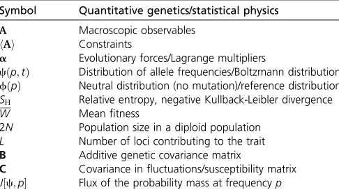
Table 2 Table of key terms and constants
Symbol Quantitative genetics/statistical physics
A Macroscopic observables
hAi Constraints
a Evolutionary forces/Lagrange multipliers
cðp;tÞ Distribution of allele frequencies/Boltzmann distribution
fðpÞ Neutral distribution (no mutation)/reference distribution SH Relative entropy, negative Kullback-Leibler divergence W Meanfitness
2N Population size in a diploid population L Number of loci contributing to the trait
B Additive genetic covariance matrix
other observables, the boundary masses also can be expressed as means of functions of allele frequency and thus treated as additional observables. The appropriate function is a character-istic functionx½a;bwhere
x½a;b¼
1 p2 ½a;b
0 else (16)
Splitting the problem domain augments the degrees of free-dom by hx½0;ei and hx½12e;1i, which control the boundary dynamics independently of the bulk dynamics and the corre-sponding Lagrange multipliers 2Nkand 2Nr. The values of k andr will be determined later. The general DynMaxEnt method, derived in Appendix E and summarized next, pro-vides a way to couple the boundary dynamics with the bulk dynamics to account for the multiscale features and resolve the technical problems of the continuous method while keep-ing the same number of degrees of freedom as the continuous DynMaxEnt.
Wefirst split the allele frequency domain into the bulk part and the boundary part and define the diffusion equation separately in the three regions in Appendix E. We couple the equations by a boundary flux that is consistent with the original diffusion equation, thus leading to the same probability mass at the boundaries as in the continuous DynMaxEnt method. The stationary distribution of the problem (E4) has the form
ceðpÞ ¼1
ℤW
2N
8 < :
e2Nke4Nm21q4Nn21 if p,e
p4Nm21q4Nn21 otherwise
e2Nrp4Nm21e4Nn21 if p.12e
(17)
with ℤ¼RceðpÞdp, whereℤis the normalization constant, and the relative masses in the three regions are determined by constantskandr. The stationary distribution (17) is not generally continuous atp¼e;12e. However, it can still be obtained by maximizing a relative entropy with a bounded base distribution
feðpÞ ¼ 1
ℤ0 8 > > < > > :
ðeqÞ21 if p,e
ðpqÞ21 otherwise
ðpeÞ21 if p.12e
ℤ0¼
Z 1
0
feðpÞdp
(18)
complemented by the following constraints on hAi and Lagrange multipliers 2Na:
A¼ ðlogW;Ue;VeÞ (19)
a¼ ðaW;m;nÞ (20)
where instead ofUandVthat diverge at the boundaries, we take their truncation top2 ½e;12e:
Ue¼
2 loge p,e
2 logp else ; Ve¼
2 logq p,12e
2 loge else (21)
The two remaining parameters,kandr, are matched to sat-isfy conditions 2 from the preceding list, leading to
k¼ 2 1
2Nlogð4NmÞ and r¼ 2 1
2Nlogð4NnÞ (22)
This relationship ensures that the approximate stationary distribution has the same proportion of the mass at the boundaries to the stationary solution of the original diffusion. Generalized to multiple loci, the MaxEnt distribution has the form
ceðpÞ ¼1
ℤW
2NYL
i¼1
8 > > > > > > < > > > > > > : 1 4Nme
4Nm21q4Nn21
i if pi,e
p4Ni m21q4Ni n21 otherwise
1 4Nnp
4Nm21
i e4Nn21 if pi.12e
(23)
withℤsuch that 1¼RceðpÞdp. We remark that the reference distributionfeðpÞis the stationary distribution in the absence of selection and mutation. Therefore, feðpÞ ¼seðpÞ21, whereseis the state-dependent diffusion coefficient:
seðpÞ ¼ 8 < :
eq p,e pq else pe p.12e
(24)
The diffusion equation in the split domain can be used to derive a new DynMaxEnt approximation for arbitrary muta-tion strengths. This is done in a manner similar to the
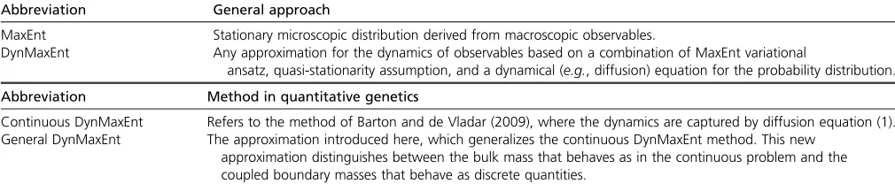
Table 3 Overview of the approximations
Abbreviation General approach
MaxEnt Stationary microscopic distribution derived from macroscopic observables.
DynMaxEnt Any approximation for the dynamics of observables based on a combination of MaxEnt variational
ansatz, quasi-stationarity assumption, and a dynamical (e.g., diffusion) equation for the probability distribution.
Abbreviation Method in quantitative genetics
Continuous DynMaxEnt Refers to the method of Barton and de Vladar (2009), where the dynamics are captured by diffusion equation (1). General DynMaxEnt The approximation introduced here, which generalizes the continuous DynMaxEnt method. This new
continuous DynMaxEnt method using the ansatz (17) and a quasi-stationarity assumption. The derivation, detailed in Appendix E, leads to the same dynamics as the original method:
@hAi
@t ¼Beða2a*Þ (25)
@a*
@t ¼ 1 2NC
21
e Beða2a*Þ (26)
where (26) is a closed dynamical system for a*. However, since constant prefactors in the stationary distribution (23) depend on mutation rates, the matrixCecontains additional
terms:
Be¼
seðpÞ 2
@Aj
@p
@Ak
@p ; Ce¼CovðAj;AkÞ 2
0W 1 2NmCov
A;x½0;eÞ
1
2NnCov
A;x½12e;1Þ
(27)
where the subtracted terms form a square matrix of the same dimension as CovðAj;AkÞ. Its leftmost columns, denoted by 0W, represent a contribution to the terms Covð;AWÞ. Because the stationary distribution (23) depends on the selection-related Lagrange multipliers only throughW2N¼eaWAW, in
a similar manner to the continuous DynMaxEnt method, all added terms are zero. In contrast, the presence of the muta-tion-related Lagrange multipliers in (23) as the scaling fac-tors results in additional terms added to Covð;UeÞ and
Covð;VeÞ, forming the remaining two columns in (27). The
components of the matricesBeandCeare functions of
effec-tive forces only, similar to the continuous DynMaxEnt approx-imation. The difference is that the expectations involve integrals through parts of the domain ½0;1 (bulk part or boundary parts), and thus the terms have to be evaluated numerically.
Applications of the General DynMaxEnt Method
In the following, we show the performance of the general DynMaxEnt method in the parameter regimes when the continuous DynMaxEnt method is not applicable because the dynamics (14) become singular. These examples involve dynamic selection and mutation in the regime 4Nm;4Nn,1. To illustrate the method step by step, we provide a pedagog-ical Mathematica notebook with the code for the general DynMaxEnt method (File S1).
Performance of the DynMaxEnt approximation for differ-ent scenarios is compared to the discrete and continuous approximations in Appendix G.
Example 1: Low and changing mutation
Here we consider a single locus under directional selection. As we show in Appendix E, this also corresponds to the case of multiple loci with equal effects. Despite its apparent simplicity,
the system still contains 2Ndegrees of freedom that capture the allele frequency distribution in a population ofNdiploid individuals. The general DynMaxEnt approximation, based on a stationary MaxEnt approximation, reduces the dynamics to a few degrees of freedom that correspond to the Lagrange multipliersa*ðtÞ. For instance, whenA¼ ðz;Ue;VeÞ, the full
dynamics in the 2N-dimensional space reduces to a three-dimensional (3D) spaceðb*;m*;n*Þ.
The general DynMaxEnt method is tested in the most challenging situation when the initially strong mutation suddenly changes to 4Nm1. The continuous DynMaxEnt method does not apply to this example for two reasons. First, when effective mutation drops below 4Nm*¼1 or 4Nn*¼1, the components of matrixBdiverge because of singularities of the stationary allele frequency distribution. Second, even when the mutation rates are keptfixed at their terminal val-ues (m*¼m,n*¼n), resulting in a reduced dynamics, the continuous DynMaxEnt method does not give correct dynam-ical predictions for small mutation rates. A closer look at the failures of the continuous DynMaxEnt method is provided in Appendix D.
The general method (withe¼1=2N) gives a satisfactory estimate of the trait mean at the beginning of the adaptation process, as shown in Figure 1, while a quick drop in effective mutation, compensated by a change in the effective selection, results in a quick loss of polymorphism. When the equilibra-tion of the effective mutaequilibra-tion is too fast, the speed of the dynamics that are limited by effective mutation becomes slower than necessary and leads to underestimation of trait mean andhUei. This can be observed over the medium
time-scalet/2N1–10.
Over long timescales, the approximate dynamics accu-rately match the exact dynamics. When we employ an addi-tional constraint on the mean heterozygosity, although noa priori selection is acting on it, we increase the number of degrees of freedom from three to four. While a general fea-ture of variational approximations is that an increase in the number of constraints leads to an improvement in the perfor-mance of the approximation, this particular choice yields a match that is almost indistinguishable in all four observables (including the addedhpqi), as shown in Figure 1.
The dynamics of Lagrange multipliers in Figure 1 (E and F) demonstrates separation of timescales. An initial quick drop in mutation n* and subsequentlym* to the vicinity of their steady states is compensated by the changes inb* (andh*) and followed by a slow relaxation ofb* (andh*) to equilib-rium once the mutation rates are barely changing. It is in-teresting that the dynamics of the effective forces differs significantly between cases E and F.
Example 2: Overdominance
intermediate peak represents an increased probability of het-erozygous individuals. We consider an analogous example to Example 1 but add initially strong selection on heterozygosity (trimodal distribution of allele frequency) that switches to a purely directional selection.
Figure 2 shows an almost perfect agreement between the exact solution and the approximation despite the fact that the approximation is not built to capture rapid switches in the forces but, to the contrary, assumes that the forces change slowly. The effective forces do not capture the rapid change in the real forces on the system but show a slow–fast relaxation to their new steady states. Appendix H shows a complemen-tary simulation when the initial (a0) and terminal conditions (a1) are switched. The system follows a different trajectory in the directiona0/a1anda1/a0.
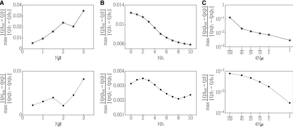
In all the simulations presented here, we use 2Ne¼1; such a thresholdecorresponds to an allele frequency of a single individual out of a population of size 2N. In Appendix F, we provide additional simulations to show that there exists an optimal thresholdNethat minimizes the approximation error. Moreover, we show that in the worst-case scenario, where a strong change in selection is coincident with a low and chang-ing mutation, the relative error of the approximation is on the order of 1%.
Example 3: Multiple loci with different effects
In this example, we show the applicability of the DynMaxEnt approximation for the evolution of quantitative traits that depend on multiple loci with different effects. The state space of the system ofLindependent loci contains essentiallyð2NÞL degrees of freedom because each locus is characterized by an
allele frequency distribution with 2Ndegrees of freedom. The reduction of the dimensionality to three (directional selec-tion) or four (overdominance) degrees of freedom thus offers an immense simplification of the problem in which instead of tracking the full allele frequency distribution we are tracking just the dynamics of the Lagrange multipliersa* correspond-ing to the underlycorrespond-ing constraints.
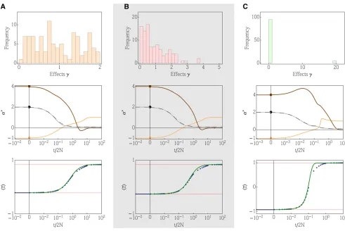
How does the method perform for different distributions of effects? A simple case, in which all effects are the same (gi¼1), coincides with Example 2 because the dynamics become the same as for a single locus (Appendix I). We consider three distinct distributions of effects to demonstrate both the effect size distributions typically assumed and also extreme examples. We chose a uniform distribution in½0;2, exponential distribu-tion with mean 1, and a bimodal distribudistribu-tion with many loci of small effect and a few loci of large effect. We chose all distri-butions to havehgi ¼1 for an easier comparison.
Figure 3 shows a comparison between the exact dynamics and the general DynMaxEnt approximation. All forces, includ-ing forward and backward mutations, were initially perturbed to a state where 4Nm¼4Nn,1, the regime where the con-tinuous approximation does not apply. When the distribution of effects was uniform or exponential, the approximation showed almost a perfect match with the true dynamics in all observed moments. Intuitively, one expects that when the dis-tribution of effects is strongly bimodal, with many small effects and a few large effects, the approximation will perform badly. This is so because the large-effect loci dominate the quick re-sponse of the system, while the small-effect loci form a second wave of adaptation at a later time that is difficult to capture by the simple approximation schemes. Figure 3 shows these two
Figure 2 Example 2: details of the general DynMaxEnt method. (A) Changes in evolutionary forces, including a rapid decrease in mutation, comple-mented by a change in selection strength and a change in the selection strength on heterozygosity. (B) The effective forcesa*. (C–F) The response of the observed quantitieshpi,hpqi,hUei, andhVei. Exact dynamics, obtained by numerically solving the diffusion equation using a discretization of space
timescales in the dynamics of Lagrange multipliers. The ap-proximation of the observables still gives a solid match, but the second wave of adaptation due to small-scale effects is not perfectly accurate anymore.
Discussion
A central result in population genetics is that the stationary distribution of allele frequencies is the product of the neutral distribution and the mean fitness raised to the power of population size: cfW2N (Wright 1937; Kimura 1955b, 1964). This result can be interpreted via an optimization principle: selection constrains the expected values of the traits that determinefitness, but the allele frequency distri-bution is distorted as little as possible by this constraint—the distortion being measured by (minus) the relative entropy. Our approximation is to assume that this MaxEnt principle holds even away from equilibrium, with the approximate distribution of allele frequencies having the stationary func-tionalformat all times. This provides a variational ansatz for
the diffusion equation and results in a set of dynamical equa-tions for the parameters of the MaxEnt distribution.
This MaxEnt approximation can be justified in the limit of slowly changing conditions. Yet, provided that mutation rates are above a critical threshold (4Nm.1), it is remarkably accurate even in the worst case, when parameters change abruptly. Even for a single locus, this approximation gives a substantial reduc-tion in complexity: the whole distribureduc-tion is described by a small number of dynamical variables that correspond directly to the forces of mutation and selection. The method extends directly to multiple loci such that the joint distribution of allele frequencies can be approximated by a small number of variables.
This paper extends the approximation to low mutation rates (4Nm,1), where the original approximation breaks down completely. The problem is that when 4Nm,1, populations are likely to be nearfixation—i.e., the distribution is concen-trated near the borders. When mutation rate or population size changes, the distribution near the boundaries changes imme-diately, whereas the distribution in the interior changes much more slowly. To see why this is so, think of the probability that
Figure 3 Example 3: dynamics of quantitative traits for 100 loci of different effects. The effects are randomly drawn from (A) uniform distribution in
a population carries one or a few copies of an allele. Because the lifetime of such rare alleles is short and is determined primarily by mutation and random reproduction, this proba-bility changes rapidly with those processes and in the short term is independent of selection or of the total population size. In contrast, the distribution of polymorphic alleles in the in-terior changes slowly with changes in mutation rate because it takes a long time for new mutations to reach high frequency or for polymorphic alleles to be lost by drift.
The MaxEnt approximation for the expectations of a set of traitshAiextends the“breeder’s equation”to include random fluctuations, mutation, and an arbitrary relation between se-lected traits and the underlying genotype. It takes the form
@thAi ¼B*ða2a*Þ(13), whereB* is a generalization of the additive genetic covariance,aare the actual forces of selec-tion and mutaselec-tion, anda* are the effective forces that would yield the same expectationshAi. Our extension is simply to modifyB* by truncating the distribution of allele frequencies within a distancee1=2Nof the boundaries, thus suppress-ing its divergence for low mutation rates. The approximation is insensitive to the location of the truncation thresholde. We give examples of directional selection and dominance; here we assume additivity across loci, but de Vladar and Barton (2011) show how the method applies to stabilizing selection, which induces pairwise epistasis between loci. We emphasize that the approximation can be applied without detailed knowledge of individual loci: only the distribution of allelic effects is needed. The approximation also can be generalized in principle to traits with linkage disequilibrium. The con-straints for such a case also would involve pairwise measures, e.g., the correlations between loci.
Like the MaxEnt approximation, the infinitesimal model (Fisher 1919, p. 403) reduces the dimensionality of the dynam-ics by following trait values rather than individual alleles. However, these approaches are quite distinct. The infinitesimal model assumes that there are so many genes that the distribu-tion of allele frequencies at each locus is hardly perturbed by selection; thus, the genetic variance that segregates within fam-ilies remains approximately constant. This is equivalent to as-suming thatNbon each allele is small (Robertson 1960). In contrast, the MaxEnt approximation can be applied to a single locus, with largeNb, and predicts the change in genetic vari-ance owing to selection. The infinitesimal model is broader, in that it describes the effects of linkage disequilibrium—though, because it assumes free recombination, these effects are only significant when selection on traits is strong; see Bulmer (1974) for an extension to allow linkage. However, if selection is weak enough that the population is at linkage equilibrium, the MaxEnt approximation will be more accurate than the infini-tesimal model because it accounts for the effects of selection on the genetic variances. Of course, this does require knowledge of the distribution of effects of alleles and their interactions.
What are the possible applications of our results? First, our results allow us to tractably predict the temporal evolution of interesting macroscopic observables, such as the trait mean or heterozygosity, even when these are determined by an
arbitrary function of a single locus or multiple loci under dynamically changing evolutionary forces. This is made pos-sible by the drastic dimensionality reduction of the MaxEnt ansatz. The examples we presented here focused on exploring this “forward prediction” scenario in regimes where previ-ously proposed approximation methods break down.
The MaxEnt approximation predicts the evolution of the allele frequency distribution—yet almost always we have only a single realization of the evolution of any one locus. However, whole-genome sequencing gives us information about the fre-quencies of alleles at very large numbers of loci. If these can be treated as independent realizations of a process common to all loci (or at least all loci in a functional class), then we can apply our method. Indeed, our assumptions are the same as those typically made in analyzing the distribution of frequencies of synonymousvs.nonsynonymous variants: each allele is taken to have an additive effect onfitness, drawn from some specific distribution. Usually, the distribution is assumed to be station-ary. However, related species that have different effective population sizes (e.g., Loeweet al.2006) or newly formed sex chromosomes (e.g., Zhouet al. 2013) require a time-dependent analysis of the kind proposed here.
Second, our results have consequences for inference of evolutionary forces from genomic and phenotypic data. The success of the MaxEnt approximation suggests that the allele frequency distribution remains close to the stationary form, even when selection, mutation, and population size are changing rapidly. This, in turn, suggests that it may be difficult to detect such changes from sequence data taken at a particular time point; note that the moments of the allele frequency distribution correspond directly to the distribution of genealogies. This is consistent with thefinding that unless selection is very strong (Nb1), it has only weak effects on genealogical structure (Williamson and Orive 2002; Barton and Etheridge 2004).
time point we were provided with the temporal profile of changing observableshAðtÞi, we could use our results to solve an inference problem and learn about the time courses of evo-lutionary forcesa.
Third, our results, together with previous relevant theoretical work, allow us to interpret the evolutionary process in informa-tion-theoretic terms. What is the meaning of entropy, beyond being simply a tool for approximation? Minus the relative entropy is the Kullback-Leibler distance, a measure of divergence from the neutral distribution. If we include mutation in the base distribu-tionf(18), then minus the relative entropy measures the de-gree to which selection concentrates populations around states of highfitness. Following Kimura (1961), entropy changes can be seen as the information about its selective history that the population can transmit (Watkins 2008). Arguably, concentra-tion aroundfit states is a better measure of adaptation than the increase in meanfitness: thoughfitness differences determine the rate of adaptation, they do not measure the outcome. Fitness mayfluctuate, and absolutefitness must stay close to zero, on average, if populations are to persist. Mustonen and Lässig (2010) derive an intriguing relation between the gain in infor-mation (equal to the reduction in entropy) and thefitnessfluxF:
2NE½F$2DS where F¼ ZT
0
X
i
biDpidt (28)
[(28) corrects a factor 2 error in Mustonen and Lässig (2010)]. This applies to a haploid population at linkage equilibrium, as assumed throughout this paper. Selection may change arbi-trarily over time so that this relation gives a lower bound on the fitnessfluxF that is required to achieve a given gain in information (i.e., reduction in entropyDS). If selection changes slowly—as required for our MaxEnt approximation to be accu-rate—then the inequality approaches an equality. Thefitness flux can be separated into a component resulting from selection (which must be positive and equal to the additive variance in fitness VW) and the remaining components, resulting from mutation and drift. Because forces other than selection are expected, on average, to act against adaptation, the latter com-ponent is negative, so the additive variance infitness should set a bound on the rate of information gain (i.e., 2NVW$2DS). Our approximation states that even out of equilibrium, the distribution of allele frequencies minimizes the information gain, subject to constraints on selected traits. By drastically reducing the dimensionality of the system to cover only the expectations of selected quantities, we can simplify expres-sions for the totalfitnessflux and variance infitness over the evolutionary trajectory and therefore may be able to under-stand how these quantities limit the amount of information that can be accumulated by selection.
Acknowledgments
We thank Harold de Vladar and Richard Kollár for helpful discussions. The research leading to these results has re-ceived funding from the European Research Council under
the European Union’s Seventh Framework Programme (FP7/2007-2013)/ERC grant agreement number 250152 (N.B.). This work was supported in part by the Human Fron-tiers Science Program (grant number RGP-0065/2012 to G.T.).
Literature Cited
Barton, N., and J. Coe, 2009 On the application of statistical physics to evolutionary biology. J. Theor. Biol. 259: 317–324. Barton, N. H., and H. P. de Vladar, 2009 Statistical mechanics and
the evolution of polygenic quantitative traits. Genetics 181: 997–1011.
Barton, N. H., and A. M. Etheridge, 2004 The effect of selection on genealogies. Genetics 166: 1115–1131.
Bialek, W., A. Cavagna, I. Giardina, T. Mora, E. Silvestri et al., 2012 Statistical mechanics for natural flocks of birds. Proc. Natl. Acad. Sci. USA 109: 4786–4791.
Bulmer, M., 1974 Linkage disequilibrium and genetic variability. Genet. Res. 23: 281–289.
de Vladar, H. P., and N. H. Barton, 2011 The statistical mechanics of a polygenic character under stabilizing selection, mutation and drift. J. R. Soc. Interface 8: 720–739.
Ewens, W. J., 2012 Mathematical Population Genetics 1:
Theoret-ical Introduction (Interdisciplinary Applied Mathematics, Vol.
27). Springer, New York.
Fisher, R. A., 1919 XV.—the correlation between relatives on the supposition of mendelian inheritance. Trans. R. Soc. Edinb. 52: 399–433.
Flegg, M. B., S. J. Chapman, and R. Erban, 2011 The two-regime method for optimizing stochastic reaction-diffusion simulations.
J. R. Soc. Interface9: 859–868.
Goeke, A., and S. Walcher, 2013 Quasi-steady state: Searching for and utilizing small parameters, pp. 153–178 inRecent Trends in
Dynamical Systems. Springer, New York.
Goldman, N., and Z. Yang, 1994 A codon-based model of nucle-otide substitution for protein-coding DNA sequences. Mol. Biol. Evol. 11: 725–736.
Hallatschek, O., 2011 The noisy edge of traveling waves. Proc. Natl. Acad. Sci. USA 108: 1783–1787.
Hick, P., and G. Stevens, 1987 Approximate solutions to the cos-mic ray transport equation the maximum entropy method. As-tron. Astrophys. 172: 350–358.
Hill, W. G., and M. Kirkpatrick, 2010 What animal breeding has taught us about evolution. Annu. Rev. Ecol. Evol. Syst. 41: 1–19. Iwasa, Y., 1988 Freefitness that always increases in evolution. J.
Theor. Biol. 135: 265–281.
Jaynes, E. T., 1957 Information theory and statistical mechanics. Phys. Rev. 106: 620.
Kimura, M., 1955a Solution of a process of random genetic drift with a continuous model. Proc. Natl. Acad. Sci. USA 41: 144. Kimura, M., 1955b Stochastic processes and distribution of gene
frequencies under natural selection. Cold Spring Harb. Symp. Quant. Biol. 20: 33–53.
Kimura, M., 1961 Natural selection as the process of accumulat-ing genetic information in adaptive evolution. Genet. Res. 2: 127–140.
Kimura, M., 1962 On the probability offixation of mutant genes in a population. Genetics 47: 713.
Kimura, M., 1964 Diffusion models in population genetics. J. Appl. Probab. 1: 177–232.
Lynch, M., B. Walshet al., 1997 Genetics and Analysis of
Quanti-tative Traits, Vol. 1. Sinauer Associates, Sunderland, MA.
McDonald, J. H., M. Kreitmanet al., 1991 Adaptive protein evo-lution at the adh locus in Drosophila. Nature 351: 652–654. Mora, T., A. M. Walczak, W. Bialek, and C. G. Callan, 2010 Maximum
entropy models for antibody diversity. Proc. Natl. Acad. Sci. USA 107: 5405–5410.
Mustonen, V., and M. Lässig, 2007 Adaptations to fluctuating selection in Drosophila. Proc. Natl. Acad. Sci. USA 104: 2277– 2282.
Mustonen, V., and M. Lässig, 2008 Molecular evolution under fitnessfluctuations. Phys. Rev. Lett. 100: 108101.
Mustonen, V., and M. Lässig, 2010 Fitnessflux and ubiquity of adaptive evolution. Proc. Natl. Acad. Sci. USA 107: 4248–4253. Plastino, A., H. Miller, and A. Plastino, 1997 Minimum Kullback entropy approach to the Fokker–Planck equation. Phys. Rev. E 56: 3927–3934.
Pressé, S., K. Ghosh, J. Lee, and K. A. Dill, 2013 Principles of maximum entropy and maximum caliber in statistical physics. Rev. Mod. Phys. 85: 1115.
Prügel-Bennett, A., and J. Shapiro, 1997 An analysis of genetic algorithms using statistical mechanics. Physica D 104: 75–114. Rattray, M., and J. L. Shapiro, 2001 Cumulant dynamics of a population under multiplicative selection, mutation, and drift. Theor. Popul. Biol. 60: 17–31.
Robertson, A., 1960 A theory of limits in artificial selection. Proc. R. Soc. Lond. B Biol. Sci. 153: 234–249.
Robinson, M., M. Flegg, and R. Erban, 2014 Adaptive two-regime method: application to front propagation. J. Chem. Phys. 140: 124109.
Schneidman, E., M. J. Berry, R. Segev, and W. Bialek, 2006 Weak pairwise correlations imply strongly correlated network states in a neural population. Nature 440: 1007–1012.
Segel, L. A., and M. Slemrod, 1989 The quasi-steady-state as-sumption: a case study in perturbation. SIAM Rev. 31: 446–477.
Sella, G., and A. E. Hirsh, 2005 The application of statistical physics to evolutionary biology. Proc. Natl. Acad. Sci. USA 102: 9541–9546. Tkaˇcik, G., O. Marre, D. Amodei, E. Schneidman, W. Bialeket al.,
2014 Searching for collective behavior in a large network of sensory neurons. PLoS Comut. Biol. 10: e1003408.
Tsimring, L. S., H. Levine, and D. A. Kessler, 1996 RNA virus evolution via afitness-space model. Phys. Rev. Lett. 76: 4440. Wakeley, J., 2008 Coalescent Theory: An Introduction, Vol. 1.
Rob-erts & Company, Greenwood Village, CO.
Watkins, C., 2008 Selective breeding analysed as a communica-tion channel: channel capacity as a fundamental limit on adaptive complexity, pp. 514–518 inProceedings of the 10th In-ternational Symposium on Symbolic and Numeric Algorithms for Scientific Computing (SYNASC’08). IEEE Computer Society, Los Alamitos, CA.
Weigt, M., R. A. White, H. Szurmant, J. A. Hoch, and T. Hwa, 2009 Identification of direct residue contacts in protein-protein interaction by message passing. Proc. Natl. Acad. Sci. USA 106: 67–72.
Williamson, S., and M. E. Orive, 2002 The genealogy of a se-quence subject to purifying selection at multiple sites. Mol. Biol. Evol. 19: 1376–1384.
Wright, S., 1931 Evolution in mendelian populations. Genetics 16: 97.
Wright, S., 1937 The distribution of gene frequencies in popula-tions. Proc. Natl. Acad. Sci. USA 23: 307.
Yang, J., B. Benyamin, B. P. McEvoy, S. Gordon, A. K. Henderset al., 2010 Common snps explain a large proportion of the herita-bility for human height. Nat. Genet. 42: 565–569.
Zhou, Q., C. E. Ellison, V. B. Kaiser, A. A. Alekseyenko, A. A. Gorchakov
et al., 2013 The epigenome of evolving drosophila neo-sex
chromosomes: dosage compensation and heterochromatin for-mation. PLoS Biol. 11: e1001711.
Appendix A: Solution of MaxEnt by the Method of Lagrange Multipliers
The variational problem
max
c SH½c ¼ 2
Z
½0;1L
cðp;tÞlog
cðp;tÞ fðpÞ
dp (A1)
withfðpÞ ¼QLi¼1ðpiqiÞ2 1
subject to constraints Z
½0;1L
cðpÞdp¼1 ; Z
½0;1L
AðpÞcðpÞdp¼ hAiobs* (A2)
[e.g., for directional selection and asymmetrical mutationA¼ ðz;U;VÞand a¼ ðb;m;nÞ] can be solved by the method of Lagrange multipliers, yielding an unconstrained maximization of a Lagrangian
L½c;l;a ¼SH½c2l 2 6 6 4
Z
½0;1L
cðpÞdp21 3 7 7
522NX
k
ak
2 6 6 4
Z
½0;1L
AkcðpÞdp2hAkiobs
3 7 7
5 (A3)
with multiplierslanda. The variational derivative of this function with respect to its argumentcis
dL½c;l;a ¼ Z
½0;1L
dc
logc
f212l22NaA
dp (A4)
and leads to a solution
cðpÞ ¼fðpÞ
ℤ e2NaA (A5)
where the normalizationℤ¼expð212lÞand the Lagrange multipliers are such that observables are correctly matched. The distributioncðpÞcoincides with the stationary solution of the Fokker-Planck equation (1) provided that theavalues are the evolutionary forces (selection, mutation) and the A values are the traits associated with the underlying processes. The evolutionary forces appear in the constrained optimization as Lagrange multipliers 2Na.
Appendix B: Matrices B and C in the Continuous DynMaxEnt Approximation
Whena¼ ðb;h;m;nÞandA¼ ðz;H;U;VÞ, the explicit form of matrixBis
B*¼
h
XL
k¼1
2 6 6 6 6 6 6 6 6 6 4
g2kpkqk 2gkp2kqkðqk2pkÞ gkqk 2gkpk
2gkp2kqkðqk2pkÞ 2p3kqkðqk2pkÞ2 2pkqkðqk2pkÞ 22p2kðqk2pkÞ
gkqk 2pkqkðqk2pkÞ 2
qk
pk 2
2
2gkpk 22p2kðqk2pkÞ 22 2
pk
qk
3 7 7 7 7 7 7 7 7 7 5
i
(B1)
as implemented in the Mathematica notebook (File S1). Because the expectationhfðpÞi ¼R½0;1LfðpÞcðpÞdpis taken over the
stationary distributioncðpÞ, which depends on the effective parametersa*, the matrixB* is also a function of the effective evolutionary forces. The components of matrix B* may be calculated using special functions, as in Barton and de Vladar (2009).
Similarly, the components of the matrixC* can be written as
C*
whereAiðpÞare functions of the microscopic allele frequencies, and after averaging over the stationary distributioncðpÞ, only the dependence on the effective forcesa* remains. Thus, the right-hand side of vector equation (14) is solely a function of effective evolutionary forcesa*, forming a system of ordinary differential equations of dimension equal to the number of observables.
Appendix C: Discrete Dynamics in the Limit of Small Nm
As 4Nmand 4Nnbecome very small, the probability distribution (7) becomes concentrated at the boundaries. The populations then switch betweenfixation for the favorable and deleterious alleles at a given locus and can be described by the fractionP, Q¼12P, of populationsfixed (or nearlyfixed) for each allele:
dP
dt ¼lþQ2l2P (C1)
The probability offixation for the favorable allele isP^¼ ½n=mþexpð24NbÞ21(Kimura 1962), and the rates of substitution of alleles by their counterparts,lþandl2, are
l2¼4Nnb e
24Nb
12e24Nb and lþ¼4Nmb
1
12e24Nb (C2)
Hence, the exact dynamics in the regime of small mutations have a form
4NdP dt ¼4Nb
4NmQ24Nne24NbP
12e24Nb (C3)
How does the standard MaxEnt approximation compare in the limit of low mutation rates? We keep mutation ratesfixed and follow a single variableP¼ hpi; we define the complementary variableb* as the selection that givesPat stationarity. In the limit of low mutation rates,
p¼ R1
0pp4Nm21q4Nn21e4Nb*ð2p21Þdp
R1
0p4Nm21q4Nn21e4Nb*ð2p21Þdp
1 4Nn
e24Nb* 1 4Nmþ
1 4Nn
(C4)
implying
e4Nb*¼4Nn 4Nm
P
Q (C5)
The same equilibrium formula is given by the ratio of substitution ratesP=Q¼lþ=l2. Under the MaxEnt approximation, the
rate of change is
4NdP
dt ¼ hpqið4Nb24Nb*Þ (C6)
Moreover, in the limit of small mutations,
hpqi ¼ R1
0p4Nmq4Nne4Nb*ð2p21Þdp
R1
0p4Nm21q4Nn21e4Nb*ð2p21Þdp
e4Nb*21
4Nb*
1 4Nmþ
e4Nb*
4Nn
(C7)
where this expression has been obtained by computing contributions to the integrals separately for each of the boundaries½0;d and½12d;1, ford1 and for 4Nm;4Nnd. Note that integration by parts has been used, resulting in the presence of the term 4Nb* in the denominator of (C7). Equation (C6) then becomes
4NdP dt ¼
4NnP24NmQ
4Nb* ð4Nb24Nb*Þ ¼ 2 6 6
4 4Nb log
4Nn 4Nm
P Q
21 3 7 7
Thus, the MaxEnt approximation to the full distribution does not converge to the exact dynamics (C3) as mutation rates become small. Nevertheless, the dynamics are approximated quite well, provided that selection is not too strong (e.g.,j4Nbj,2). The MaxEnt approximation greatly underestimates the rate of change at the margins and gives no effect of selection at the extreme allele frequencies (see Figure C1, left).
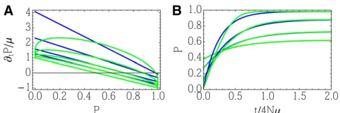
Figure C1 Discrete MaxEnt approximation. (A) The exact rate of change, obtained from the discrete model (C3) (blue), compared with the MaxEnt approximation (C8) (green) in the limit of small 4Nm¼4Nn;Nb¼0;0:5;1;2;4 (bottom to top) and 2N¼1000. Rates are scaled relative to the neutral mutation rate, assumed to be symmetrical (m¼n). (B) Dynamics following an abrupt switch from 4Nb¼20:5;21;22;24 to the reverse.
However, the equilibria necessarily agree: the exact and the approximate rates of change are zero at the same point. The right plot in Figure C1 shows the exactPðtÞand the MaxEnt approximation; these are close to 4Nb¼62, but the solution becomes poor for 4Nb¼4 (upper pair of curves). The MaxEnt solution is accurate for 4Nb #2 becausePremains within the interior [1=ð1þe2Þ ¼0:112,P,0:888), where the rate of change is approximated well.
Appendix D: Failure of the Continuous DynMaxEnt for 4Nm,4Nn <1
The log meanfitness typically will be a sum over moments of allele frequencies. For example, a selection gradientbon a trait with mean z¼2Pigiðpi2qiÞ will introduce a component where aW¼b and AW¼z; a model with dominance requires aW¼ ðb;hÞandAW¼ ðz;HÞ, and epistasis introduces mixed second-order moments of the allele frequencies. Thus, the matrix
Bis an expectation over polynomial functions of allele frequencies and is well behaved.
In contrast, the elements ofBthat describe mutation diverge when 4Nm,1 or 4Nn,1. To see this, consider a single locus for whichA¼ ðz;H;U;VÞ ¼ ð2p21;2pq;2 logp;2 logqÞ, and the elementsB3;3,B3;4, andB4;4areh2q=pi,h22i,h2p=qi(B1). Thus,B3;3diverges when 4Nm,1, andB4;4diverges when 4Nn,1. If we can assume that mutation rates arefixed, then we can avoid the difficulty either byfixing the mutation rates always at their actual values (i.e.,m¼m*,n¼n*) or by choosing a reference distribution that includes mutation,e.g.,f¼Qkpk4Nm21q4Nn21
k , and dropping the observablesUandV. These two approaches are equivalent becausefixing the mutation rate leads to@thzi ¼B1;1ðb2b*Þ þB1;2ðh2h*Þ, leading to the same dynamics forb* andh* as if the reference distribution included mutation.
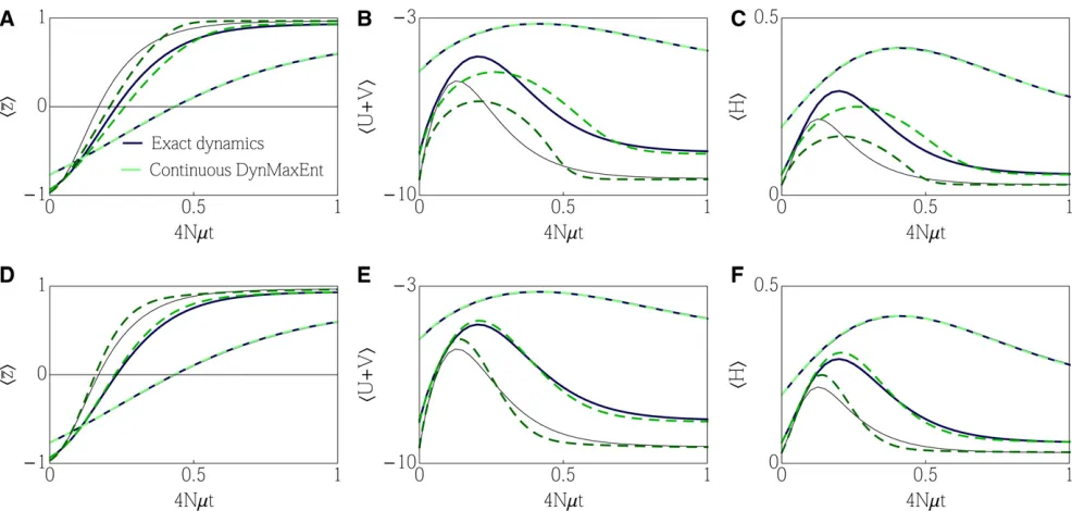
Wefirst explore the continuous DynMaxEnt approximation for 4Nm.1 and compare its accuracy with that for 4Nm,1. We study the worst-case scenario when a selection suddenly changes sharply fromNb¼ 24 toNb¼4; this is by no means an adiabatic change. Mutations equal 4Nm¼4Nn¼2;1=2;1=4, where thefirst choice (4Nm.1) allows a full continuous DynMaxEnt approximation including constraints on hUi andhVi, while the second and third choices require afixed instantaneous mutation rate and constraints on hUi and hVi dropped to keep the entries of the additive covariance matrixBfinite. Figure D1 (top row) shows the predicted observableshzi,hUþVi, andhHiestimated by the continuous DynMaxEnt method for each of the mutation rate alternatives compared with the exact solution, while keeping the het-erozygosityfixed throughout the simulation (not employing the constraint onh2pqi). The method is accurate for 4Nm¼2 (where the mutation rate also changes dynamically) but shows significant deviations from the true dynamics for 4Nm¼4Nn¼1=2;1=4.
Figure D1 Failure of the continuous DynMaxEnt approximation for strong selection. Dynamical response to a fast change in selectionNb¼ 24 to Nb¼4 for symmetrical mutation rates that are unperturbed and 2N¼1000. Each panel shows three simulations with mutation rates 4Nm¼4Nn2 f2;1=2;1=4g(light-green to dark-green) where the exact observables (black) are compared with the continuous DynMaxEnt approxi-mation (green, dashed). (A–C) Simulation with constraintshzi,hUi, andhViwhen 4Nm;4Nn.1 and a single constrainthziwhen 4Nm;4Nn,1. (D–F) Simulation with constraintsz,hHi,hUi, andhViwhen 4Nm;4Nn.1 and two constraintshziandhHiwhen 4Nm;4Nn,1.
Figure D2 Effective coefficients
a*of the continuous DynMaxEnt approximation for the scenario of Figure D1. (A) 4Nm¼4Nn¼2, (B) 4Nm¼4Nn¼1=2, and (C) 4Nm¼4Nn¼1=4 are compared between the simulation without (solid line)vs.with (dashed line) the heterozygosity as a degree of freedom. The population size is 2N¼1000.
introducing additional constraints onh2pqi. This is visible both for 4Nm.1, where the number of Lagrange multipliers was increased from three to four, and for 4Nm,1, where the constraint onhziwas complemented by the second constraint on a mean heterozygosityhHi ¼ h2pqi.
Figure D2 presents the dynamics of Lagrange multipliers in the example in Figure D1, where a sudden change in selection fromNb¼ 24 toNb¼4 was applied to three systems with different mutation ratesNm; Nn2 f2;1=2;1=4g. While in the superthreshold regime 4Nm; 4Nn.1, the mutation is allowed to change in the continuous DynMaxEnt approximation; in the subthreshold regime 4Nm; 4Nn,1, it isfixed.
Figure D2 suggests that increasing the number of constraints; which increases the dimensionality of the problem, is associated with a slower convergence to a steady state and a separation of timescales. This is visible both for 4Nm.1 (left), where the number of Lagrange multipliers was increased from three to four, and for 4Nm,1, where the constraint onhziwas complemented by the second constraint on a mean heterozygosityhHi ¼ h2pqi.
with the stationary form, but polymorphism decays more slowly, so the full distribution is not from the stationary class. The continuous DynMaxEnt method fails to capture the true dynamics because the mutation rates have to be instantly adjusted to the terminal values.
Figure D3 shows that three measures of diversity (hUi;hVi;hpqi) change rapidly, withhUi and hVifalling most rapidly because they are more sensitive to the rapid changes near the boundary thanhpqi. Note thathUi ¼ h2 logpifalls untilt1=2N because probability accumulates close top¼0 (note the log scale in Figure D3) but then increases again more slowly as favorable mutations substitute, transferring probability away fromp0. The mean changes rapidly and substantially while
Figure D3 Failure of continuous DynMaxEnt approximation for changing mutations 4Nm,1 and 2N¼1000. (A) Changes in evolutionary forces that draw the system out of equilibrium include a rapid decrease in mutation, complemented by a change in selection strength. (B, D, and E) The response of the observed quantitieshpi,hUi, andhVi. (C) The initial andfinal stationary allele frequency distributions. (F) The effective forcesa*.
heterozygosity is still high but then changes more slowly aftert1=2N, when the genetic variance is low and selection is limited by the influx of new mutations.
The changes in effective parametersa* are shown in Figure D3F. Because we assume that the population is initially in its stationary state, these parameters necessarily begin at their actual values (4Nm*,4Nn*¼2,Nb*¼ 21=2). After the mutation rate decreases, the probability of beingfixed increases rapidly, and therefore, 4Nm* and 4Nn* fall quickly, approaching their new values byt=2N0:1;m* fallsfirst because the probability of being nearp¼0 increases faster than the probability of being nearp¼1. Over this time,Nb* changes even while the meanhpihardly changes in order to compensate for changingNmand Nn. At later times, when the effective mutation rates are constant and close to their actual (low) rates,Nb* increases as the mean changes.
Fixing the effective mutation rates makes DynMaxEnt unable to capture transient properties of the adaptation process. The dynamics of the mean allele frequency followp9¼2hpqiðb2b*Þ, whereb* can be obtained at each time as a value that gives the current mean allele frequency givenm*¼mandn*¼n. The effective directional selection can be used further to compute the change of observables, as displayed in Figure D3 (dashed blue). This continuous DynMaxEnt approximation fails to capture transient dynamics of the observed quantities but still converges to the correct state. If the exact dynamics are followed for a short time from the switch of the evolutionary forces and only then is the continuous DynMaxEnt approximation initialized, the approximation would more closely agree with the actual observables. This is so because the real dynamics of the trait mean slow down in time as the system gets close to an equilibrium and therefore are better captured by an approximate process whose speed of adaptation is limited by the smallfixed mutation rate.
Appendix E: Derivation of the General DynMaxEnt Approximation for Low Mutation from the Diffusion Equation 1