http://dx.doi.org/10.4236/ojdm.2014.42007
The Paired Assignment Problem
Vardges Melkonian
Department of Mathematics, Ohio University, Athens, USA Email: [email protected]
Received 18 January 2014; revised 17 February 2014; accepted 16 March 2014
Copyright © 2014 by author and Scientific Research Publishing Inc.
This work is licensed under the Creative Commons Attribution International License (CC BY).
http://creativecommons.org/licenses/by/4.0/
Abstract
We consider a variation of the maximum bipartite matching problem where each completed task must have at least two agents assigned to it. We give an integer programming formulation for the problem, and prove that the basic solutions of LP-relaxation are half-integral. It is shown that a fractional basic solution can be further processed to obtain an optimal solution to the problem.
Keywords
Matching Problems, Linear Programming, Basic Solutions, Graph Algorithms
1. Introduction
1.1. Problem Definition
We are given a bipartite graph =
(
,)
where each edge e∈ has one endpoint in and the other endpoint in . Elements of are normally referred as agents (or people), and elements of are referred as tasks (or jobs). Then a→ ∈t means that agent a can perform task t (not every agent can perform every task). In classic maximum bipartite matching problem the goal is to find a matching in (a set of pairwise non-adjacent edges) that contains the largest possible number of edges. A matching is a one-to-one assignment: each agent can be assigned to at most one task, and each task can be assigned to at most one agent.We consider the following variation of the maximum bipartite matching problem. Each agent still can be assigned to at most one task. But in our problem a task can be completed only if at least two agents are assigned to it. The goal is to maximize the number of completed tasks.
The problem can be given by the following integer program (IP):
max j
j J y
∈
∑
(1). . pj 1, for each , j J
s t x p P
∈
≤ ∈
2 , for each ,
pj j
p P
x y j J
∈
≥ ∈
∑
(3), binary, for each , .
pj j
x y p∈P j∈J (4)
Here is the set of agents, is the set of tasks. yj is a binary variable which is equal to 1 if task j is completed. xpj is a binary variable which is equal to 1 if agent p is assigned to task j. The objective of Function (1) is trying to maximize the number of completed tasks. Constraint (2) provides that each agent is assigned to no more than one task. Constraint (3) provides that if a task is completed then at least two agents are assigned to it.
1.2. Applications
The problem was first considered in [1] as a solution method for a combinatorial problem related to circuit re- duction. [1] gave an integer program for the problem. In this paper we give a more efficient solution method based on the LP-relaxation of the integer program.
A few typical examples of the problem are given below. A group has members (agents) who should be as- signed to projects (tasks). Each member can work only on some of the projects based on her/his qualifications. A project can be pursued only if at least two members are assigned to it. The goal is to maximize the number of projects that are pursued.
In a variation of the facility location problem, potential facility sites are the tasks, and demand points are the agents. Not every potential facility can serve every demand point (based on distance, compatibility, etc.). It is economical to open a facility only if it is assigned to serve at least two demand points. The goal is to maximize the number of open facilities.
Another possible situation is in the following. A company should assign guides to several tourist groups (tasks). Each group is from a certain country and needs guides who speak their language. The company has sev-eral guides (agents); each guide speaks sevsev-eral languages. Each group should be assigned two guides (primary and backup) satisfying the language requirement. The goal is to maximize the number of possible assignments.
1.3. Literature Review
Matching and assignment problems are of great importance in graph theory and combinatorial optimization ([2] [3] [4]). The history of development, applications and solution methods of matching and assignment problems are discussed in [4]. Some variations of matching problems are discussed in [5]. A survey of assignment prob- lems is given in [6]. In most variations the goal is to find a one-to-one assignment subject to some kind of re- strictions. But some variations allow assignments of multiple agents to the same task or multiple tasks to the same agent ([7]-[9]). The generalized assignment problem ([8]) allows an agent to do multiple tasks provided that the set of tasks assigned to an agent do not exceed its capacity. In [7] an agent can be assigned several tasks, and the goal is to find an assignment that minimizes the total time of completing all the tasks.
Our model was introduced in [1]. To the best of our knowledge, no other model has considered the variation that a task can be completed only if two or more agents are assigned to it.
1.4. Our Results
The maximum bipartite matching problem can be solved by network flow techniques. It can be formulated as a maximum flow problem and solved by the augmenting path algorithm. Another solution method is linear pro- gramming. The constraint matrix of its integer program is totally unimodular, and thus the LP-relaxation returns integer solutions.
1.5. Outline of Paper
The paper is structured as follows. In Section 2, we show that any basic solution of the LP relaxation of (IP) is half-integral. In Section 3, we show how the basic solutions can be further processed to increase the number of completed tasks. In Section 4, we give an algorithm for solving the paired assignment problem and show that it returns an optimal solution. Future directions are discussed in Section 5.
2. Description of Basic Solutions of LP-Relaxation
The linear programming relaxation (LP) of the integer program (IP) is obtained by replacing the binary requirements of xpj and yj with 0≤xpj ≤1 and 0≤ yj ≤1 .
Theorem 1 Basic solutions of (LP) are half-integral. Specifically, every x variable is integerpj , and every
j
y variable takes value 0, 0.5, or 1.
Proof: Suppose the functional constraints of (LP) are rewritten in a standard form Av≤b. The coefficient matrix of Constraints (2) and (3) has the following form:
0 C
D F
where
• C represents the coefficients of xpj variables in Constraints (2); • D represents the coefficients of xpj variables in Constraints (3); • F represents the coefficients of yj variables in Constraints (3).
Matrix C D
is totally unimodular because each column has exactly one 1 and one –1. Matrix F is a diagonal matrix with 2’s on the main diagonal.
Suppose B is a basis matrix for the augmented form of Av≤b. Then the corresponding basic solution can be computed as follows:
( )
1
det adj
v=B b− =B b B
.
Next we evaluate det
( )
B . First we expand by the columns of slack variables; in the result all the rows that correspond to basic slack variables will be crossed out. Then we expand by the columns of yj variables. Consider the following cases.Case 1. Suppose we expand by a column of a yj variable that takes a fractional value in the basic solution. Then the slack variables of both yj≤1 and −yj ≤0 are basic, and thus both rows were crossed out in earlier expansions. So there is only one non-zero entry left in the column of yj, namely 2 in corresponding Constraint (3). Thus, the expansion will result in 2 times the corresponding cofactor.
Case 2. Suppose we expand by a column of a yj variable that takes value 1 in the basic solution. Then the slack variable of −yj ≤0 is basic, and thus the corresponding row was crossed out earlier. There are two non-zero entries in the column of yj: 2 in corresponding Constraint (3) and 1 in yj ≤1. The minor of entry 2 is 0 since after crossing its column only 0's are left in the row of yj≤1. Thus, the expansion will include only one non-zero term, which is 1 times the corresponding cofactor.
Case 3. Suppose we expand by a column of a yj variable that takes value 0 in the basic solution. Then the slack variable of yj≤1 is basic, and thus the corresponding row was crossed out earlier. There are two non-zero entries in the column of yj: 2 in corresponding Constraint (3) and –1 in −yj ≤0. The minor of entry 2 is 0 since after crossing its column only 0's are left in the row of −yj ≤0. Thus, the expansion will include only one non-zero term, which is -1 times the corresponding cofactor.
The matrix obtained after crossing out all basic yj columns with corresponding rows is totally unimodular as a submatrix of a classic assignment problem. Thus, based on Cases (1)-(3), det
( )
B is either 2k or −2k where k is the number of yj variables that take fractional values in the basic solution.Next, for each different type of variable, we evaluate adj
B b and the value of the variable. Consider a basic variable xpj.
here, and the cofactor of e is either 2k
or −2k
. Then the corresponding additive term in B badj is 0, 2k , or 2k
− since we have only 0's and 1's in b.
Suppose e is an element in the column of xpj in a constraint of type (3). The right-hand side of the constraint in the standard form is 0. Thus, the corresponding additive term in B badj is also 0.
Summarizing, all the additive terms in B badj are 0, 2k
, or −2k
. Thus, xpj can take only integer values since det
( )
B is either 2kor −2k . Consider a basic variable yj.
Suppose e is an element in yj’s column. Submatrix Be obtained by crossing its column and row has only one 2 less than the original matrix B. Thus, if we repeat the analysis done in Cases (1)-(3) for Be we can have the following possible values for its determinant: 2k
or −2k
if yj takes an integer value, 2k−1 or
1
2k−
− if yj takes a fractional value. Then the corresponding additive term in B badj is 0, 2k , −2k
, −2k−1 , or −2k−1
since we have only 0’s and 1’s in b. Thus, the only values yj can take are 0, 0.5, and 1 since
( )
det B is either 2k
or −2k .
3. Increasing Number of Completed Tasks by Reassignment
Suppose we have a solution to (LP). Based on Theorem 1, each yj variable takes one of the following values, 0, 0.5, or 1. Correspondingly, we distinguish three types of task-nodes in the current solution.
Definition 1 A task-node is called • completed if the corresponding yj=1; • incomplete if the corresponding yj=0.5; • unassigned if the corresponding yj =0.
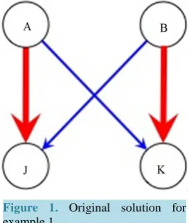
[image:4.595.245.382.553.715.2]Suppose we have a half-integral solution. It would be reasonable to include the completed tasks in the solution. But simply including the completed tasks might not give a good solution. Consider the example 1 of
Figure 1. We will have the following convention for the rest of paper. Any arc that takes value 1 in the LP-relaxation will be called red arc and will be colored red (bold) in our figures; any arc that takes value 0 in the LP-relaxation will be called blue arc and will be colored blue in our figures. In the example of Figure 1, an optimal basic solution has no task with two agents assigned to it (both yJ and yK are 0.5). But we can clearly have one completed task by assigning both A and B to J as it is done in Figure 2.
In order to increase the number of completed tasks we need a reassignment from the current solution. The following result provides a general strategy for such a reassignment.
Lemma 1 Any reassignment that increases the number of completed tasks will decrease the number of incomplete tasks by at least two.
Proof: Suppose there are k completed and l incomplete tasks in the current solution with LP-value 0.5
k+ ×l. Recall that k+0.5×l is the optimal value of the LP-relaxation. Suppose there is another solution with at least k+1 completed tasks. Since the LP-value of any feasible solution cannot be more than k+0.5×l then the number of incomplete tasks in the new solution is no more than 2×
(
k+0.5× −l) (
k+1)
= −l 2. Lemma 1 implies that incomplete tasks should be the key in any reassignment that increases the number of
Figure 2. Reassigned solution for example 1.
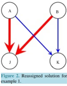
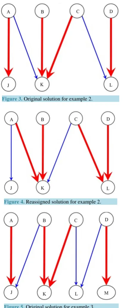
completed tasks. To get some insight how such an increase can be achieved consider example 2 given in Figure 3 and Figure 4 and example 3 given in Figure 5 and Figure 6.
In Figure 3, tasks J and L are incomplete, and task K is completed. By reassigning agents, as it is done in Figure 4, L becomes completed and J unassigned, thus increasing the number of completed tasks from 1 to 2.
InFigure 5, tasks J and M are incomplete, task K is completed, and L is unassigned. By reassigning agents, as it is done in Figure 6, J and L become completed, and K and M become unassigned, thus increasing the number of completed tasks from 1 to 2.
We need the following definition to discuss the common pattern in the above examples.
Definition 2 Let A→J and A→K be two arcs with the same agent-node A as origin. If in a current solution A→J is red (assigned) and A→K is blue (unassigned) then we call J← →A K a red-blue arc pair.
All our examples, where we were able to create more completed tasks by reassignment, have the following feature. There are two incomplete tasks which are connected by a sequence of red-blue arc pairs. The number of completed tasks is increased by recoloring those red-blue pairs of arcs: the red arcs become blue, and the blue arcs become red. Recoloring the arcs essentially means reassigning every agent-node in the sequence to a different task.
In example 2, the original sequence is J← →A K← →C L which becomes J← →A K← →C L after recoloring. In example 3, the sequence is J← →B K← → ←C L D→M which becomes
J← →B K ← → ←C L D→M after recoloring.
The increase in number of completed tasks happens because the task-nodes in sequences change their statuses. In our examples, an unassigned task becomes assigned (e.g., task L in example 3); incomplete nodes can become completed (e.g., task L in example 2) or unassigned (e.g., task J in example 2); completed tasks can become unassigned (e.g., task K in example 3) or stay completed (e.g., task K in example 2).
But we do not have a completed task-node with both incident arcs blue in the original sequence. It would mean that the two agents assigned to the task are not in the sequence. Thus, by recoloring we would assign two more agents to a task which is already completed. In that case it is unlikely that we would increase the number of completed tasks by reassignment.
The above analysis of the patterns observed in our examples leads to the following important concept. Definition 3 A sequence P of red-blue arc pairs, that connects two incomplete task-nodes, is called a valid path if
• there are no interior incomplete nodes on P;
• any interior completed node on P has at least one incident red arc in the sequence.
Using the concept of valid path, the following result generalizes the strategy of increasing the number of completed tasks observed in our examples.
Theorem 2 If there is a valid path connecting two incomplete task-nodes in a half-integral solution then we can increase the number of completed tasks by 1 by recoloring all the arcs on the path.
Figure 3. Original solution for example 2.
Figure 4. Reassigned solution for example 2.
Figure 5. Original solution for example 3.
First we categorize the task-nodes on P, and describe how recoloring will change their statuses.
1) If u is an unassigned node then it has two incident blue arcs on P. Thus, recoloring will make both arcs red, and u will become a completed node (e.g., task L in example 3).
2) If u is an incomplete node and its incident arc on P is blue then recoloring the arc will make u completed (e.g., task L in example 2).
3) If u is an incomplete node and its incident arc on P is red then recoloring the arc will make u unassigned (e.g., task J in example 2).
Figure 6. reassigned solution for example 3.
5) If u is a completed node with one incident red arc and one incident blue arc on P then after recoloring u will stay completed with one incident blue arc and one one incident red arc on P (e.g., task K in example 2).
Note that we cannot have a completed node with two incident blue arcs on P since P is a valid path. As discussed above, only type (5) nodes do not change their status in the result of recoloring. Thus, our goal is to find out how status changes in other type of nodes affect the number of completed tasks on P. To answer that question we need to discuss the possible configurations of type (1)-(4) nodes on P.
Suppose u and v are task-nodes of type (1)-(4) on P. We say u and v are P-neighbors if all the internal task-nodes (if any) on the subpath of P joining u and v are type (5) nodes. Based on the definition of type (5) nodes, any two neighboring arcs on the subpath joining two P-neighbors have different colors. Also, based on their definitions, type (1) and (2) nodes have only incident blue arcs on P while type (3) and (4) nodes have only incident red arcs on P. Based on the last two observations, we have the following intermediate result.
Lemma 2 Any node of type (1) or (2) can be a P-neighbor only with a node of type (3) or (4), and conversely, any node of type (3) or (4) can be a P-neighbor only with a node of type (1) or (2). In other words, on P, type (1) or (2) nodes are alternated by type (3) or (4) nodes.
Now we are ready to discuss how the number of completed tasks will be changed in the result of recoloring. We have three possible cases.
Case 1: Both incomplete nodes i1 and i2 on P are of type 3. Based on Lemma 2, the number of type (1) nodes on P is more than the number of type (4) nodes on P exactly by 1. After recoloring, incomplete nodes i1 and i2 become unassigned, each type (1) (unassigned) node becomes completed, and each type (4) (completed) node becomes unassigned. Thus, the number of completed nodes is increased exactly by 1.
Case 2: Both incomplete nodes i1 and i2 on P are of type 2. Based on Lemma 2, the number of type (4) nodes on P is more than the number of type (1) nodes on P exactly by 1. After recoloring, both i1 and i2 become completed, each type (1) (unassigned) node becomes completed, and each type (4) (completed) node becomes unassigned. Thus, the number of completed nodes is increased exactly by 1.
Case 3: One of i1 and i2 is of type 2, and the other one is of type 3. Based on Lemma 2, the number of type (4) nodes on P is equal to the number of type (1) nodes on P. After recoloring, the incomplete node which is of type (2) will become completed, each type (1) (unassigned) node becomes completed, and each type (4) (completed) node becomes unassigned. Thus, the number of completed nodes is increased exactly by 1.
Summarizing, in any case the number of completed nodes is increased exactly by 1. This concludes the proof of theorem 2.
4. Algorithm for Paired Assignment Problem
The result of Theorem 2 is the basis of the following algorithm for solving the paired assignment problem. Algorithm 4.1 Algorithm for Paired Assignment
In the next two subsections we show that: 1) a valid path can be found efficiently using a modified version of breadth-first search (BFS); 2) the algorithm returns an optimal solution for the problem.
4.1. Procedure for Finding a Valid Path
We need to define an auxiliary digraph to do the search. For each red-blue pair of arcs J← →P K we define a directed arc J←K connecting the task-nodes by choosing the direction of the red arc. Let be the set of all directed arcs defined this way (note that two directed arcs J←K and J←L might have their original blue-red pairs sharing the red arc). Then we have a digraph =
(
,)
defined on the set of all tasks . For example, the digraph corresponding to the original graph of Figure 5 is J→K← →L M .The search of a valid path can be done in . The equivalent of a valid path in D is an undirected path P connecting two incomplete nodes such that
• there are no interior incomplete nodes on P;
• any interior completed node on P has at least one of its incident arcs incoming.
The modified BFS for finding a valid path in is done as follows. One of the incomplete nodes, say I, is chosen to be the root node. The modification to BFS concerns the completed nodes in the queue.
• If a completed node C is reached from its parent-node K in the queue through an incoming arc K→C then C is marked as fully visited and the search continues from C as in standard BFS. Namely, after all the nodes reached from C by an arc, incoming or outgoing, are included in the queue we dequeue C and do not consider it again in the search (as suggested by its name).
• If a completed node C is reached from its parent-node K1 in the queue through an outgoing arc K1←C then C is marked as partially visited. At this point, a node L can be considered a child of C and included in the queue only if it is reached from C through an outgoing arc L→C. But C is not dequeued yet; we allow to visit it again. If at some point in the search it is visited from a node K2 through an incoming arc K2→C then C becomes fully-visited and the search from it is continued as in standard BFS described above.
We quit the search when
1) either another incomplete node J is found; in this case the output is a valid path connecting I and J; 2) or no other incomplete node is found and there are only partially visited nodes left in the queue; in this case I is not connected to another incomplete node by a valid path.
4.2. Optimality of the Algorithm Output
We claim that algorithm 4.1 returns an optimal solution for the original problem (IP), based on the following result.
Theorem 3 If there is no valid path connecting any two incomplete task-nodes then the number of completed tasks cannot be increased. Thus, Algorithm 4.1 returns an optimal solution for the paired assignment problem.
Proof: The proof is by induction on the number of task-nodes.
Basis step. The theorem statement is clearly true for any graph with only one task-node. Inductive step.
Inductive hypothesis. Assume that the theorem statement is true for any graph with less than n task-nodes. That is, for any graph with less than n task-nodes, if
• assignment S represents an optimal solution of (LP),
• there is no valid path connecting any two incomplete task-nodes in S, then S has maximum possible number of completed tasks.
We need to prove the same for any graph with n task-nodes. Suppose an instance of the problem is given by a graph with n task-nodes. Let S1 be a solution for ,
• corresponding to an optimal solution of (LP), • and with no valid paths connecting incomplete nodes.
Let S2 be a different solution that is obtained by reassigning some agents. Let the number of completed tasks in S1 be M. We need to prove that the number of completed tasks is no more than M in S2.
If none of incomplete and unassigned tasks in S1 becomes completed in S2 then the number of completed tasks clearly cannot be increased. So we need to consider the following two cases.
2) An unassigned node in S1 becomes completed in S2. Case 1: Node i is incomplete in S1 and becomes completed in S2.
Get a reduced graph ′ from by deleting task-node i and the two agent-nodes p and q assigned to i in S2. Denote the reduction of S1 in ′ by S1′, and the reduction of S2 in ′ by S2′.
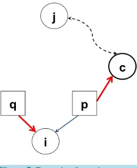
Let c be the node from which i is getting its second assignment in S2. Namely, suppose task-node p was assigned to c in S1 and is reassigned to i in S2 (see Figure 7). Note that c cannot be an incomplete node in S1; otherwise c← →p i would be a valid path connecting incomplete nodes i and c in S1. Thus,
c is a completed node in S1, and becomes incomplete in S1′. We can state the following about S1′.
1) The number of completed tasks in S1′ is M−1 since it was M in S1 and c was completed in S1 but incomplete in S1′.
2) S1′ is an optimal solution to the linear program for the reduced graph ′ based on the following reason. We cannot have another assignment S2′ with larger LP-value for ′; otherwise, by adding p→i and
q→i to S2′, we could get an assignment with larger LP-value for original .
3) We cannot have c connected to an incomplete node j in S1′ by a valid path jc; otherwise jc← →p i would be a valid path connecting incomplete nodes i and j in S1. Thus, there are no valid paths connecting two incomplete task-nodes in S1′ since we didn't have any in S1 and c is the only new incomplete task in S1′ compared to S1.
Based on (2) and (3), the conditions for inductive hypothesis hold for S1′. Thus, we can claim that the number of completed tasks cannot be increased in the result of reassignment from S1′ to S2′. Then, based on (1), the number of completed tasks in S2′ is at most M−1, and the number of completed tasks in S2 is at most M when we add i to the completed tasks of S2′.
Case 2: Node u is unassigned in S1 and becomes completed in S2.
Get a reduced graph ′ from by deleting task-node u and the two agent-nodes p and q assigned to u in S2. Denote the reduction of S1 in ′ by S1′, and the reduction of S2 in ′ by S2′.
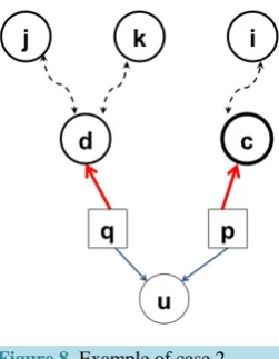
Let c and d be the nodes from which u is getting its assignments in S2. Note that c and d cannot be both incomplete in S1; otherwise we would have a valid path between c and d through the unassigned node u (Figure 8). Then we might have the following two subcases.
Subcase 2.1: c is completed and d is incomplete in S1.
Then, after deleting agent-nodes p and q with their assignments to c and d, c becomes incomplete and d becomes unassigned in S1′.
We can state the following about S1′.
1) The number of completed tasks in S1′ is M−1 since it was M in S1 and c was completed in S1 but incomplete in S1′.
2) S1′ is an optimal solution to the linear program for the reduced graph ′ based on the following reason. We cannot have another assignment S2′ with larger LP-value for ′; otherwise, by adding p→u and
[image:9.595.245.383.539.708.2]q→u to S2′, we could get an assignment with larger LP-value for original .
Figure 8. Example of case 2.
3) We cannot have c connected to an incomplete node i by a valid path ic in S1′; otherwise ic← → ← →p u q d would be a valid path connecting incomplete nodes i and d in S1 (see Figure 8). We also cannot have two incomplete nodes j and k connected by a valid path jk that has d as an interior unassigned node in S1′; otherwise jd would be a valid path connecting incomplete nodes j and d in S1 (Figure 8). Thus, there are no valid paths connecting two incomplete nodes in S1′.
Based on (2) and (3), the conditions for inductive hypothesis hold for S1′, and we can claim that the number of completed tasks cannot be increased in the result of reassignment from S1′ to S2′. Then, based on (1), the number of completed tasks in S2′ is at most M−1. Hence the number of completed tasks in S2 is at most
M when we add u to the completed tasks of S2′. Subcase 2.2: Both c and d are completed in S1.
Then, after deleting agent-nodes p and q with their assignments to c and d, both c and d become incomplete in S1′.
We can state the following about S1′.
1') The number of completed tasks in S1′ is M−2.
2') S1′ is an optimal solution to the linear program for the reduced graph ′ based on the following reason. We cannot have another assignment S2′ with larger LP-value for ′; otherwise, by adding p→u and
q→u to S2′, we could get an assignment with larger LP-value for original .
3') We cannot have both c and d connected to two different incomplete nodes i and j in S1′ by valid paths ic and d j; otherwise ic← → ← →p u q d j would be a valid path connecting incomplete nodes i and j in S1. But we might have one of c and d connected to an incomplete node in
1
S′ by a valid path, or c and d connected to each other by a valid path in S1′. Based on (3'), further division into cases is needed.
Subcase 2.2.1: Suppose none of c and d is connected to an incomplete node in S1′ by a valid path. Then there are no valid paths connecting two incomplete nodes in S1′, and based on (2'), the conditions for inductive hypothesis hold for S1′. Hence the number of completed tasks cannot be increased in the result of reassignment from S1′ to S2′. Then, based on (1'), the number of completed tasks in S2′ is at most M−2. Thus, the number of completed tasks in S2 is at most M−1 when we add u to the completed tasks of S2′.
Subcase 2.2.2: Suppose c is connected to an incomplete node in S1′ by a valid path (that incomplete node could be d itself). Then after recoloring all the arcs on the path the number of completed tasks will increase by 1. Let S1′′ be the solution obtained from S1′ by recoloring the arcs on the valid path.
We can state the following about S1′′.
1'') The number of completed tasks in S1′′ is M−1 since it has one more completed task than S1′. 2'') S1′′ is an optimal solution to the linear program for the reduced graph ′ since it is obtained from S1′ by recoloring the arcs on a valid path which is not changing the LP-value.
3'') There are no more valid paths joining two incomplete nodes in S1′′.
(1''), the number of completed tasks in S2′ is at most M−1. Hence the number of completed tasks in S2 is at most M when we add u to the completed tasks of S2′.
Thus, we proved that the number of completed tasks cannot be increased in any of the above cases. This completes the proof of Theorem 3.
5. Future Directions
Below are some possible future directions.
It would make sense to consider the weighted version of the problem. Weights could be associated with the arcs (to make it a variation of the assignment problem) or/and with the nodes.
It is interesting whether there is a purely combinatorial algorithm for solving the problem (without using linear programming).
A generalization of the paired assignemnt problem could be the following: task i can be done only if at least
( )
f i agents are assigned to it.
• The special case when f i
( )
=1 for every task i is the classic maximum matching problem. • Our problem is the special case when f i( )
=2 for every task i.• The problem for general f i
( )
might be hard to solve.References
[1] Melkonian, V. (2011) Circuit Integration through Lattice Hyperterms. Discrete Mathematics, Algorithms and Applica-tions, 3, 101-119.
[2] Ahuja, R., Magnanti, T. and Orlin, J. (1994) Network Flows: Theory, Algorithms, and Applications. Prentice Hall, En-glewood.
[3] Alevras, D. (2009) Assignment and Matching. Encyclopedia of Optimization, 1, 106-108. [4] Lova’sz, L. and Plummer, M.D. (1986) Matching Theory. North-Holland, Amsterdam.
[5] Goddard, W., Hedetniemi, S.M., Hedetniemi, S.T. and Laskar, R. (2005) Generalized Subgraph-Restricted Matchings in Graphs. Discrete Mathematics, 293, 129-138. http://dx.doi.org/10.1016/j.disc.2004.08.027
[6] Pentico, D. (2007) Assignment Problems: A Golden Anniversary Survey. European Journal of Operational Research, 176, 774-793.
[7] Aora, S. and Puri, M.C. (1998) A Variant of Time Minimizing Assignment Problem. European Journal of Operational Research, 110, 314-325. http://dx.doi.org/10.1016/S0377-2217(97)00266-X
[8] Cattrysse, D.G. and Van Wassenhove, L.N. (1992) A Survey of Algorithms for the Generalized Assignment Problem.
European Journal of Operational Research, 60, 260-272.