A New Quantum Radial Wavelet Neural Network Model
Applied to Analysis and Classification of EEG Signals
Saleem M. R. Taha,
Ph.D. Department of Electrical Engineering College of Engineering, University of BaghdadJadiryah, Baghdad, Iraq
Abbas K. Nawar,
M.Sc. Department of Electrical Engineering College of Engineering, University of BaghdadJadiryah, Baghdad, Iraq
ABSTRACT
In this paper, a new model of multi-level transfer function radial wavelet neural network using quantum computing is achieved. This model is applied to analyze and classify the electroencephalographic (EEG) signals. The independent component analysis (ICA) is used as processing after normalization of these signals. Some features are extracted from the data using the clustering technique (CT). A new factor that combines the accuracy and the time of classification is suggested to evaluate the performance of the proposed model with other previous models. This factor represents the accuracy to time ratio (ATR). The average accuracy of the proposed quantum radial wavelet neural network (QRWNN) model is 90.5619125% at 50 minutes. The ATR value is 1.8112, which shows the superiority of the proposed model.
General Terms
Pattern Recognition, Theory, Algorithms
Keywords
EEG Signals, Neural Networks, Quantum Computing, Radial Basis Functions, Wavelet Transforms, Radial Wavelet Neural Networks
1.
INTRODUCTION
In the 1990s the concept of quantum neural network (QNN) was developed. It is based on quantum mechanics to overcome the shortcomings and inadequacies of traditional neural network model. Since then, many researchers in different fields made their QNN model. It is based on multi-incentive function making use of quantum superposition state in quantum theory. This QNN model has been successfully used in many applications giving high classification results in pattern recognition with uncertainty and cross-data.
The quantum wavelet neural network (QWNN) model has been introduced [1]. It is a neural network with multi-resolution based on the wavelet analysis theory and the theory of quantum superposition. The incentive function of the hidden layer in QWNN model uses non-linear wavelet instead of the non-linear sigmoid function in QNN. The superposition of selected wavelet function is called multi-wavelet incentive function. The QWNN model has advantage in accuracy and generalization ability for pattern classification.
This paper proposed a new quantum radial wavelet neural network (QRWNN) model. It combines Gaussian wavelet basis function with radial basis function and quantum neural network. Then it is applied to a very important application of analysis and classification of electroencephalographic (EEG) signals. The main advantage of the proposed QRWNN model is the capability to independently reveal the having of
uncertainty in the sample data and adaptively learn to quantify the existing uncertainty and reducing the computation processes during the training process, thus reducing the time of classification.
The EEG examination is a standard procedure in the study of all forms of cerebral disease. Its use in the study of patients with seizures and those suspected of having seizures becomes essential [2]. The EEG consists of a set of multichannel signals. The pattern of changes in signals indicates brain activities. There are five categories of these signals: delta, theta, alpha, beta, and gamma. Each of which is associated with a certain activity of the brain.
2.
THE PROPOSED QUANTUM
RADIAL WAVELET NEURAL
NETWORK MODEL
Radial basis functions (RBFs) are embedded into a two-layer feed forward neural network (FFNN), such a network is characterized by a set of outputs. Each unit of the hidden layer implements a radial activated function. The output units implement a weighted sum of hidden unit outputs. In pattern classification application the input represents feature vectors, and the output corresponds to a class. QRWNN is a new field which combines the QNN with radial wavelet (RW). A motivation for using QRWNN is that the concept (quantized) is used to develop the hidden units of these networks. According to the idea of quantum state superposition, transfer function of neurons in the hidden layer is expressed as linear superposition multi-level transfer function leading to reduce the quantum interval. Hence, the classification has more freedom. Another advantage is that the input weights are cancelled, as well as the number of neurons in the hidden layer is reduced. Therefore the number of output weights becomes small.
The proposed QRWNN consists of inputs, one layer of multilevel hidden nodes, and output nodes. Let the only synaptic weight connecting the ith output nodes to the jth hidden nodes be . Let
, where m is the number of the feature vectors of data set X. Suppose a multilevel hidden unit has discrete quantum levels. Its activation function can be written as a superposition of activation functions, each shifted by . Gaussian wavelet has been chosen to serve as an adaptation basis function to network’s hidden layer.
= (1)
(2) Where is activation function, is a slope factor, and
widths of the multi-level activation function, called the quantum intervals, are determined by jump-positions . The input to the jth hidden unit from kth feature vector is
. Therefore response of the jth multi-level hidden
node to the kth feature vector can be written as
T .
= (3)
=
Therefore response of the jth multi-level hidden node to the kth feature vector can be written as
(4)
The output vector of output layer is
(5)
The general model of the QRWNN is
(6)
Where k is sample number.
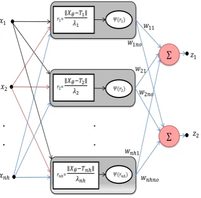
[image:2.595.55.252.447.641.2]The linear partition generated by an additional hidden unit has all the degree of freedom to align itself along any direction on the feature space. On other hand, the activation function within multi-level hidden nodes transfer function can only “spread-out” or “collapse-in” parallel to each other [3]. Figure 1 shows the structure of the QRWNN.
Fig 1: Quantum radial wavelet neural network structure.
3.
A GRADIENT-DESCENT-BASED
LEARNING ALGORITHM FOR THE
QRWNN
The assumed underlying algorithm is easily calculated, best for large data sets. Convergence between these learning algorithms based on rate . If they are too large (such as
constant) oscillation may occur. If they are too small, may not move far enough to reach a local minimum [4]. This can be done in two ways: on-line learning or example-by-example, in which the weights out are adjusted after every training
pattern; and batch or off-line learning, in which learning (weight adjustment) occurs after all of the training examples have been presented to the network once [5].
The learning of QRWNN parameters is considered in two steps. The synaptic weights out need to be update first in order to train the QRWNN to consistently partition the feature space of the given data set. Simultaneously, the uncertainty present in the feature space must be learned through the adaptation of the parameters .
3.1
Updating the Weights out of QRWNN
Let be the desired output vector for the input feature vector . Let be the actual output. A gradient-descent-based algorithm for learning the synaptic weights of the QRWNN can be derived by minimizing the quadratic error function sequentially for each .
with .
Where is the actual output of the training pattern and output . is desired output of the training pattern and output . is the total number of the training pattern. E are mean square error functions.
The weights out are adjusted after each feature vector
so that is minimized, this method is called example-by-example or on-line learning. The advantages of this method are [4]:
It requires less computation per step.
Randomization may help escape poor local minima.
The parameters are updated by minimizing objective
function .
(7)
Where = .
At any epoch , adjustment of parameters are performed.
3.2
Updating the Quantum Intervals
The quantum intervals of quantum neurons in the hidden layer can be learned by minimizing the class-conditional variances at the output of hidden nodes. On other hand quantum intervals can be learned by a minimal output variety of hidden layer neuron based on the same data category of sample data. The output of variance for class is [5]
(8)
Where
and it represents the sum of outputs of hidden neurons for all the inputs that belong to class divided by the number of samples in that class.
=
=
=
.
.
.
.
The adjustment of quantum intervals will be realized by minimizing objective function G.
(9)
The update equation for can be obtained by setting the change in , say proportional to the gradient of G with respect to as
(10)
(11)
Where = .
According to Equations (10) and (11), the adjustment formula of is:
(12)
Where is the learning ratio of
Algorithm: Training The QRWNN
The 1st step in the QRWNN classifier algorithm is to initialize all the parameters according to the above equations.
Update the synaptic output weights: For k=1,2,…,m
For j=1,2,…,
For s=1,2,…,
=
For i=1,2,….,
For i=1,2,…,
Update the quantum intervals For k=1,2,…,
For k=1,2,…,
For s=1,2,…,
=
For j=1,2,…,
For k=1,2,…,m For j=1,2,…,
For s=1,2,…,
4.
DATA SELECTION
From the data available at [6], the whole database consists of five EEG data set (denoted A-E), each containing 100 single channel EEG signals of 23.6 seconds from five seprate classes. Sets A and B consisted of signals taken from surface EEG recordings of five healthy volunteers with eye open and eye closed, respectively. Signals in set C and set D were recorded in seizure-free intervals from five epileptic patients from the hippocampal function formation of the opposite hemisphere of the brain and from within the epileptic zone, respectively. Set E contains the records of five epileptic patients during seizure activity. All EEG recordings were made with the same 128-channel amplifiers system, using an average common reference. The recorded data was digitised at 173.61 samples per second using 12-bit resolution. Band-pass filter setting were 0.53-40 Hz (12dB/oct). The amplitude of EEG recordings are given in micro volt [7].
5.
CLASSIFICATION OF EEG SIGNAL
The classification of EEG can be divided into three parts. Part one is to process raw EEG signals by removing all noise and artifacts, but preserving all the characteristics of the original signal. As well as cleaning the signal from the influence of the reference electrode, if one is used [8]. Independent Component Analysis (ICA) is the best method to accomplish all of these, since the EEG data are non-Gaussian, non-linear, and non-stationary [9].Part two is feature extraction by cluster technique (CT). Feature extraction is the process of extracting useful information from the signal. Features are characteristics of a signal that are able to distinguish between normal and abnormal cases of EEG signals. The requirements for feature extraction are [8]:
Reducing the size of the data by selecting appropriate features.
Preserving all information from the signal that is needed for classification.
The CT method is proposed for feature extraction from the original EEG database. It is conducted in three steps as follows:
Step 1: Each EEG data is divided into n groups, which are called clusters with specific time interval.
Step 2: Each cluster is partitioned into m sub-clusters with a specific duration.
Step 3: Eight statistical features are extracted from each sub-cluster data point. The statistical features are minimum, maximum, mean, median, first quartile range, third quartile range, inter-quartile range and standard deviation of the EEG data.
Part three is EEG signal classification by QRWNN model. Where the obtained features are employed as the input to the proposed QRWNN model.
6.
EXPERIMENTS ON EEG SIGNALS
The epileptic EEG data has five sets, Set A to Set E, and each set contains 100 channel of data. Every channel consists of 4069 data points with 23.6 seconds. Each channel data is normalized and then divided into 16 groups where each group is called cluster and each cluster consists of 256 data points of 1.475 seconds. Then every cluster is again partitioned into sub-clusters. Each sub-cluster contains 64 observations of 0.3688 second. Eight statistical features are calculated from each sub-cluster. These features are the input for each of five different classification techniques, namely: Feed Forward Neural Network (FFNN), Quantum Neural Network (QNN), Wavelet Neural Network (WNN), Quantum Wavelet Neural Network (QWNN), and finally the Quantum Radial Wavelet Neural Network (QRWNN).
The number of elements of each pair has been divided into two parts:
First part is used for training network called training samples. These samples usually take 70% from data. The data sample is sent through the network to find and then calculate error and accuracy of training data.
Second part is used for testing network called testing samples. These samples take the remaining 30% of data. The testing samples are tested by the above methods and the error and accuracy of testing data are calculated.
The performance of a particular run of the program, or a particular reading by an expert was evaluated in terms of the accuracy of the classification. This accuracy represents the per cent of the ratio of the total number of correct classifications to the total number of testing samples.
7.
RESULTS
In this work the patterns for training and testing processes are chosen randomly. Training is conducted until the standard of error fell below 0.0001. The mean square error denotes the error limit to stop QRWNN training.
A three layer structure of QRWNN is applied. It consists of 32 inputs, 2 outputs, 10 hidden layer nodes and 2 quantum intervals. The slope factor of multi-level transfer function is chosen to be 0.4 by trial and error. The learning rate for weight adjusting is set to 0.5.
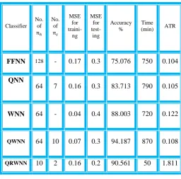
For QRWNN the average accuracy of 90.561% is obtained after 500 iterations. The average Mean Square Error (MSE) is 0.16 and time of the training process is 50 minutes. Table 1 shows the results of the five classification techniques.
[image:4.595.307.564.269.522.2]In order to evaluate the performance of the proposed QRWNN model with the other models (FFNN, QNN, WNN, and QWNN), a comparison factor is proposed. It represents a trade-off between the time taken for classification and the accuracy of it. This factor represents the classification accuracy to classification time ratio and is denoted as (ATR). As the value of ATR becomes high that refers to a better performance. The ATR value of QRWNN classifier is 1.811, while its values for FFNN, QNN, WNN and QWNN are 0.104, 0.105, 0.122 and 0.108, respectively. That shows the superiority of the QRWNN model.
TABLE 1. Comparison of EEG classification results
Classifier No.
of No.
of MSE
for
traini-ng
MSE for test-ing
Accuracy %
Time
(min) ATR
FFNN 128 - 0.17 0.3 75.076 750 0.104
QNN
64 7 0.16 0.3 83.713 790 0.105
WNN 64 - 0.04 0.4 88.003 720 0.122
QWNN 64 10 0.07 0.3 94.187 870 0.108
QRWNN 10 2 0.16 0.2 90.561 50 1.811
8.
DISCUSSION
An epileptic EEG data is used in this work to test the performance of the proposed QRWNN model. All calculations are performed using MATLAB (version 7.12.0.635). 2240 vectors are used for training and 960 vectors for testing.
function sense provides considerable flexibility in designing the QRWNN model. The other advantage of QRWNN over QWNN is the reduction of the number of neurons in the hidden layer which could lead to a little computation, 10 hidden nodes for QRWNN but 128 hidden nodes for FFNN and 64 hidden nodes for QNN, WNN and QWNN. This means reducing the total number of parameters (input weights, output weights, and jump position) to be learned.
9.
CONCLUSION
In this paper a QRWNN model with Gaussian wavelet as an incentive function is proposed for classification of EEG signals. Because EEG signals possess a combination of slow variations over long periods, with sharp transient variations over short periods, wavelet neural networks are more natural choice than other mainstream neural networks for EEG analysis. Thus, the main contribution of this work is the development of a new QRWNN model for the analysis and classification of EEG signals. It has been found that using quantum neurons instead of traditional neurons and radial features are often able to learn faster. The other advantage of QRWNN is the reduction of the hidden layer nodes leading to a little computation. The results of the experiments demonstrated that the proposed QRWNN model has the best performance by having the highest value of ATR compared to FFNN, QNN, WNN and QWNN EEG classifiers. The ATR factor represents a compromise between classification accuracy and time of classification. Thus, its value provides a performance indication of different techniques. The ATR value of QRWNN is greater than its values of FFNN, QNN, WNN and QWNN by 17.41, 17.24, 14.84 and 16.76 times, respectively. In addition, we can choose the suitable basis function for the data in QRWNN making it more flexible than the rest.
10.
REFERENCES
[1] Taha, Z. K. 2012 Quantum Neural Network Model with Wavelet Theory. M. Sc. Thesis. Electrical Engineering Dept., University of Baghdad.
[2] Ropper, A. H. and Brown, R. H. 2011 Adams and Victor’s Principles of Neurology, 8th
edition.
[3] Karayiannis, N. B. and Purushothaman, G. 1997. Quantum neural networks (QNN’s): inherently fuzzy feed forward neural networks, IEEE Transactions on Neural Networks, vol. 8, no. 3.
[4] More on Regression Gradient Descent Classification. COMP-652 Lecture 2, September 6, 2005. Available: http://www.facweb.litkgp.ernet.in/~sudeshna/courses/
[5] Mahdi, A. A. H. 2010 The Application of Neural Network in Financial Time Series Analysis and Prediction Using Immune System. M. Sc. Thesis. School of Computing and Mathematical Sciences, Liverpool John Moores University.
[6] EEG Time Series (epileptic data). 2005. Available: http://www.meb.Unibonn.de/epileptologie/science/physi kleegdata.html
[7] Siuly, Y. L. and Wen, P. 2010. Analysis and classification of EEG signals using a hybrid cluster technique. In Proceedings of the IEE/ICME International Conference on Complex Medical Engineering, Gold Cost, Australia, July 13-15, pp. 34 – 39.
[8] Horlings, R. 2008. Emotion Recognition Using Brain Activity. Man-machine Interaction Group, Delft University of Technology, Faculty of Electrical Engineering, Mathematics, and Computer Science.