Interference Mitigation in Cognitive Radio using Genetic Algorithm

Interference Mitigation in Cognitive Radio using

Genetic Algorithm

Soma Chakraborty

School of Electronics Engineering, KIIT University,

Bhubaneswar-751024, Odisha, India

Rashmi Deka

School of Electronics Engineering, KIIT University,

Bhubaneswar-751024, Odisha, India

Jibendu Sekhar Roy

School of Electronics Engineering, KIIT University,

Bhubaneswar-751024, Odisha, India

ABSTRACT

In order to improve the spectrum utilization, cognitive networks have been proposed. A cognitive network can reuses the spectrum of licensed user in a way such that the services of the licensed users are not disrupted harmfully. This paper presents the optimization of interference generated by a secondary network to a primary network for a cognitive radio (CR) networks using genetic algorithm (GA).The interference model used for optimization, in cognitive radio networks, is presented employing power control. A power control scheme is studied to govern the transmission power of a CR node. The probability density functions (PDFs) of the interference received at a primary receiver from a CR network are first studied numerically and then under the control scheme the interference distributions are fitted by log-normal distributions with reduced complexity. In GA optimization, the chromosome’s genes correspond to the adjustable parameters in a given radio, and the chromosomes are genetically manipulated so that GA can find a set of parameters that optimize the radio according to the user’s current needs.

General Terms

Interference, spectrum sharing radio, power control, genetic algorithm.

Keywords

Cognitive radio, Shadowing, Hidden node, Probability distribution function (PDF).

1.

INTRODUCTION

With the increasing demand and growth in wireless services over the past few years, the spectrum is becoming more and more congested especially in the bands below 3GHz. With the requirement to improve spectrum utilization, the newly emerging cognitive radio (CR) technology has attracted increasing attention [1-3]. A CR network is envisioned to be capable of reusing the unused or underutilized spectra of current systems by sensing its surrounding environment and adapting its operational parameters autonomously. Cognitive radio tries to take advantage of the unused spectrum of the licensed (primary) users [4, 5]. In addition to spectrum sensing algorithms, sharing protocols, policies, among other things, the interference management has become important in cognitive radio, in order to manage and fulfill the regulatory constraints. To treat and quantify interference produced by the unlicensed users at the licensed receivers, management of interference is required [6, 7]. In order to manage this interference, the cognitive (secondary) users must be able to adjust their parameters to fulfill these constraints.

In the paper, an interference model for cognitive radio (CR) networks employing power control scheme is studied to illustrate the effect that the different parameters produce on the interference in the licensed bands. The distribution of the interference power at a primary receiver is studied when the interfering secondary terminals are distributed in a Poisson field. A power control scheme is studied to govern the transmission power of a CR node. Further, for power control scheme, their interference distributions are fitted by log-normal distributions, which reduce computational complexity compared to a numerical approach to obtain PDFs [8-10]. Here, Genetic Algorithm using MATLAB is used as the optimization tool. Some parameters are optimized in order to mitigate interference in a cognitive radio network. The impacts of ε (minimum distance between the static receiver and an interferer), shadowing, and small scale fading on the probability density function (PDF) of the interference power is investigated. Moreover, the effect of imperfect static system knowledge & hidden node on the interference experienced at the receiver is also investigated.

2.

INTERFERENCE

CONTROLLING

BEHAVIOR

AND

SYSTEM

MODEL

Interference in the context of CR networks can be classified into two types: intra-network interference and inter-network interference [6].Intra-network interference, also known as self-interference, refers to the interference caused within one network. Some examples of intra-network interference include inter-symbol interference in frequency-selective channels and multi-access interference (MAI) in multiuser networks. It exists to some extent in every wireless communication system, and there are a number of techniques to mitigate them efficiently. On the other hand, inter-network interference refers to the mutual interference between the primary and CR networks (interference from CR to primary networks and vice versa).

Cognitive behaviour may be divided into three categories: Interference avoiding behaviour, interference controlling behaviour and interference mitigating behaviour [11-15].

2.1

System Model

P (k) =exp (-λA)(λA)k/k! (1)

Interference is caused to the static or primary receiver by secondary networks that transmit in the same frequency band as the static radio. Interference between static radios is not taken into consideration. The interference power at the static receiver is modeled as a random variable [16, 17]. The path loss function is

g (rj)=rj -α

(2)

where, rj is the distance between the jth (j = 1, 2…) active CR transmitter and the primary receiver and α is the pathloss exponent. If α is not greater than 2, the sum interference power at a receiver would be a function of the network size and would be infinite for an infinite sized network.

For secondary networks without any interference region, we have ε = 0 and consequently g(R)→∞. With a typical value of the pathloss exponent β = 4, following similar steps in we can obtain the closed-form expression of the PDF of Y as [8, 17]

fy (y)=(π/2)λy -3/2

e- π³λ²/4y (3)

The above PDF falls into the category of Levy distribution S1/2(σ, 1, μ) with the scale parameter σ =π

3_λ2

/2 and the shift parameter μ = 0.

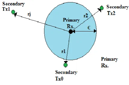
Fig 1: A primary receiver having a region of interference of radius ϵ surrounded by secondary transmitters.

2.2

Modeling the Interference Statistic at the

Static Receiver

The static receiver is at the center of a circular region with radius a (that extends to infinity). Interfering radios are uniformly distributed in this region with intensity n per unit. The minimum distance between the static receiver and an interferer is assumed to be greater than some positive value ε > 0. Hence the region has an inner-radius ε. The normalized interference power at the static receiver from this annular region is then,

X (n, ε,α)=∑J(n, ε,α) g(r) (4)

Here, J (n, ε, α) is the set of interfering radios with density n in the annular region with radius r such that ε ≤ r ≤ a. The sum of

random variables is asymptotically log-normal under certain conditions. These conditions shown to be satisfied for the sum of received powers from interferers uniformly distributed in a circular region with a non-zero inner-radius. In addition, simulation results show that the distribution of the interference statistic X (n, ε, α) is heavy-tailed. The log-normal distribution is heavy tailed, positively skewed and is suitable to model random variables that are constrained by zero but have a few very large values. Measurements and experimental results have also shown that out-of-cell interference can be well-approximated by a log-normal distribution [16]. Taking into account these observations and the fact that fit tests support it, X (n, ε, α ) is modeled as a log-normal random variable. A cumulant-matching approach is used for the modeling.

The probability density function of a log-normal variable is

p(x)=(1/xσ√2π)exp(-(ln(x/m))2_/2σ2₎ (5)

Parameters m and σ are given by m1 = m exp (0.5 σ2

) and m2 = m2 exp (σ2) (exp (σ2) - 1). Here, mk is the k th cumulant of X (n, ε, α) and is calculated.The moment generating function (MGF) of X (n, ε, α) is first derived to calculate the first two cumulants. The derivation is based on the method used in to calculate the characteristic function of X (n, 0, α).

When characteristics of the interference statistics are investigated to derive desirable features for SS schemes the kth cumulant of the interference statistic at the static receiver when interfering radios are distributed in an annular region with ε < r < ∞ is [17]

mk=(2nπ/(kα-2)) Px k _{1/ ε} kα-2 (6)

Here, n is the density and Px is a scaling factor for the transmit power of interfering spectrum sharing radios. The kth cumulant decreases linearly with a reduction in n, exponentially with a reduction in Px and exponentially (as a factor α) with an increase in ε. A reduction in the variance narrows the density distribution and translates to faster decay of outage probabilities with increasing tolerable interference powers.

2.3

Impact of Shadowing

The effect of small-scale fading in addition to log-normal shadowing was also investigated via simulations and analysis. However, it was found that the interference is dominated by log-normal shadowing and the inclusion of small-scale fading does not significantly alter the results.

The kth _{cumulant of X}

shad (n, ε, ∞) is therefore given by [17]

Mk (Xshad(n, ε,∞))=2nπeσl²c²k²/2_{/(kα-2)( ε} kα-2

) (7)

Again the distribution of Xshad (n, ε, ∞) is fitted to a lognormal distribution. This is similar to the use of a log-normal to model the sum of randomly-weighted log-normal variables.

2.4

Hidden Node Problem

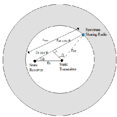
Let ras be the range from the static transmitter within which the SS radio can identify static radio transmissions and let θ be the angle of the line joining the SS radio transmitter and the static receiver w.r.t. the line joining the static transmitter and receiver. These variables are illustrated in Figure 2. Consider a disc of radius a. Then the area outside the sensing region is given by π(a2

-ras 2

). rmin (θ) is the minimum distance of the agile

transmitter from the static receiver such that the static transmitter is hidden from it. It is a function of θ and is given by

rmin(θ)=rscosθ + rassin(cos

-1

(rssinθ/ras))

(8)

Fig 2: CR transmitters distributed in the shaded region which is the hidden node region around a static transmitter

Let ε (θ)=max {rmin(θ),rphy}. The interference statistic at the static receiver for a spectrum sharing scheme employing interference avoidance in the absence of perfect system knowledge is given by

(9)

In case of imperfect sensing SS radios attempt to locate static radio receivers and static radio transmissions by either sensing signals from the static receivers or by sensing transmissions from static transmitters.

In either scenario, sensing errors might occur and interference could be caused at the static receiver by an individual SS radio transmission. Hence, unlike the perfect system knowledge scenario, an outage can be caused at the static receiver by an individual SS radio interferer in addition to an outage caused by the sum of received powers from SS radio interferers. The probability of sensing error (pse), increases as the distance

between the radio transmitting the signal and the SS radio increases and can be modeled as

Pse(r) =Crq; rphy≤ r ≤ rse

(10)

1; r > rse

Here, C is some weighting constant such that at distance rse

between the SS radio and the radio transmitting the signal to be sensed, Pse (rse) = 1 (C =1/rseq). q is a factor which can be used

to shape the distribution of pse. It is assumed that sensing error is

directly proportional to the path-loss, i.e., q = α.

The static receiver is assumed to transmit a signal indicating a static radio transmission in a particular frequency band. The probability of a SS radio, making an error while sensing this signal, is assumed to be given by pse (r), where r is the distance

between the SS radio and the static receiver. Thus in addition to the interference caused by radios outside the circular region with radius rmin, interference is caused at the static receiver by radios

inside the circular region that make an error in sensing the signal from the static receiver.

The interference statistic can now be re-written as

(11)

A radio in the annular region with inner-radius rphyand

outer-radius a (the number of radios is Poisson distributed with intensity measure n) interferes with the static radio with a probability of pres (r). This new distribution of interfering radios

can be modeled by a thinning operation on the original Poisson distribution where a point of the original Poisson process is retained with probability pres (r) that depends upon the distance r

from the centre of the circular region. The kth _{cumulant m}

k of is therefore given by

(12)

3.

APPLICATION

OF

GENETIC

ALGORITHM

TO

INTERFERENCE

MITIGATION

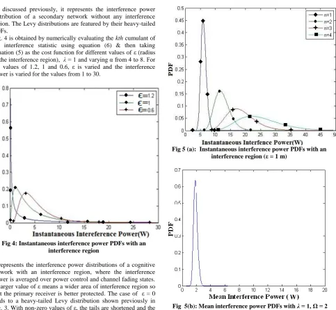
Using Genetic Algorithm MATLAB different parameters are taken and optimized. Taking equation (3) as the cost function the PDF of Y is evaluated numerically. The instantaneous interference (Y) is varied for the values 1 to 100 and the density parameter (λ=L) is varied for the values shown below. Fig. 3 shows the Levy distribution based on equation (3) with different values of λ (L) at interference region being zero i.e. ε = 0.

As discussed previously, it represents the interference power distribution of a secondary network without any interference region. The Levy distributions are featured by their heavy-tailed PDFs.

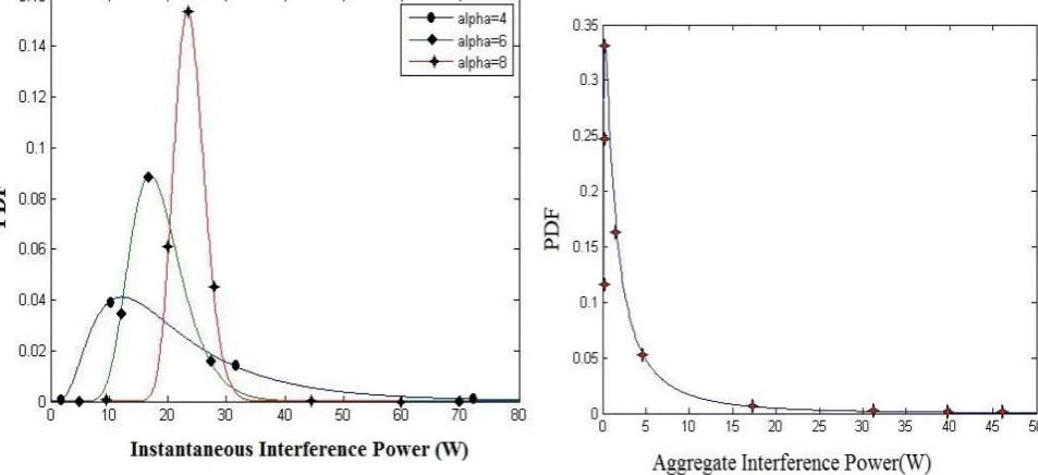
Fig. 4 is obtained by numerically evaluating the kth cumulant of the interference statistic using equation (6) & then taking equation (5) as the cost function for different values of ε(radius of the interference region), λ = 1 and varying α from 4 to 8. For the values of 1.2, 1 and 0.6, ε is varied and the interference power is varied for the values from 1 to 30.

Fig 4: Instantaneous interference power PDFs with an interference region

It represents the interference power distributions of a cognitive network with an interference region, where the interference power is averaged over power control and channel fading states. A larger value of ε means a wider area of interference region so that the primary receiver is better protected. The case of ε= 0 leads to a heavy-tailed Levy distribution shown previously in Fig. 3. With non-zero values of ε, the tails are shortened and the distribution of the interference power tends to be more confined. In Fig. 5, we assume ε = 1 m and show the impacts of the terminal density λ and average transmit power Ω on the interference power distribution. Moreover, with the increasing λ, the mean of the interference power scales linearly with λ, whereas the variance increases slower than a linear scale. The average transmit power Ω has a scaling effect on the interference Y. When Y follows a Gaussian distribution, both the mean and variance would be scaled by Ω to the same degree. The difference of the scaling effects of λ and Ω can be seen by comparing the two distributions obtained with (λ = 2, Ω = 1) and (λ = 1, Ω = 2), both scaled from that with (λ = 1, Ω = 1). The two distribution curves have roughly the same mean but a smaller variance is observed for the former case.

Fig 5 (a): Instantaneous interference power PDFs with an interference region (ε = 1 m)

Fig 5(b): Mean interference power PDFs with λ = 1, Ω = 2

Fig 6: Instantaneous interference power PDFs with an interference region (λ = 1)

It is seen that the PDFs in Fig. 6 has slightly heavier tails than that in Fig. 4. This is because that when the effects of fading and shadowing are taken into account, there is a higher probability that a strong and dominant interference would occur.

Fig 7: Instantaneous interference power PDFs with different power control exponents α with an interference region under

different fading scenarios (ε= 1.4 m, λ = 3)

It can be seen from Fig. 7 that (i) both the mean and variance of the accumulated interference are significantly reduced when adopting the power control scheme; (ii) introducing interference region also reduces the interference experienced at the primary receiver; (iii) increasing the power control exponent α leads to the decrease of interference.

Fig 8(a): Aggregated interference power PDFs with perfect system knowledge

Fig. 8(a) shows aggregated interference power for Log-normal approximation for interference distribution with perfect system knowledge taking α=4, λ=3 and for a hidden primary receiver under power control.

Fig 8(b): Aggregated interference power PDFs with hidden primary receiver

Fig 9: Aggregated interference power PDFs for perfect primary receiver knowledge and for Log-normal approximation for interference distribution with a hidden

primary receiver under power control

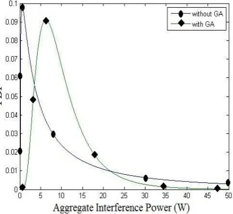
Fig. 10 shows the aggregate interference power for a perfect primary system knowledge using GA and without using GA. Fig. 11 shows the aggregate interference power for an imperfect primary system knowledge using GA and without using GA.

Fig 10: Aggregated interference power for perfect system knowledge

In Fig. 10 & fig. 11 it is observed that with GA, the tails are shortened and the distribution of the interference power tends to be more confined. It is seen that the increase in interference caused at the static receiver without GA tends to be greater as compared to the plot with GA.

Fig 11: Aggregated interference power for an imperfect system knowledge

4.

CONCLUSION

The distribution of the interference generated by a secondary network to a primary network has been optimized here using MATLAB genetic algorithm. Secondary terminals are assumed to be cognitive so that they can cease the transmission if any primary receiver within a distance of ε is detected. The characteristic function of the random interference is studied taking into account the cognitive ability, power control, and channel fading. Interference modeling from CR transmitters to a primary receiver when the knowledge of the primary receiver is imperfect, i.e., the hidden primary receiver problem is also done. Using GA, when more than one parameter is optimized it is found that the mean and the variance of the probability distribution function are reduced.

5.

REFERENCES

[1] Mitola J. 1999. Cognitive radio for mobile multimedia communications, IEEE International Workshop on Mobile Multimedia Communications, pp. 3-10.

[2] Federal Communication Commission, Spectrum policy task force report, Washington DC, FCC 02-155, 2 Nov. 2002.

[3] Federal Communication Commission, Facilitating opportunities for flexible, efficient, and reliable spectrum use employing cognitive radio technologies, NPRM & Order, ET Docket No. 03-108, FCC 03-322, 30Dec. 2003.

[4] Federal Communications Commission, Unlicensed operation in the TV broadcast bands, ET Docket No. 04-186, 2004.

[5] Rieser C.J. 2004. Biologically inspired cognitive radio engine model utilizing distributed genetic algorithms for secure and robust wireless communications and networking. Ph.D. dissertation, Virginia Polytechnic Institute and State University.

Interference Cancelation and Management Techniques, IEEE Vehicular Technology Magazine, vol. 4, no. 4, pp. 76-84.

[7] Subhedar M. and Birajdar G. 2011. Cognitive Radio Networks: A Survey,International Journal of Next-Generation Networks (IJNGN) vol.3, no.2, pp. 12-16.

[8] Hong X., Wang C.X. and Thompson J.S. 2008.Interference modeling of cognitive radio networks, Proc. IEEE VTC’08-spring, Singapore, pp. 1851–1855.

[9] Timmers M., Pollin S., Dejonghe A., Bahai A., Van der Perre L. and Catthoor F. 2008. Accumulative interference modeling for cognitive radios with distributed channel access, Proc. IEEE CrownCom’08, Singapore.

[10] Chen Z., Wang C.X., Hong X., Thompson J., Vorobyov S.A. and Ge X. 2010. Interference modeling for cognitive radio networks with power and contention control," Proc. IEEE Wireless Comm. or Networking Conf., WCNC'10, Sydney, Australia, pp. 1-6.

[11] Devroye N., Mitran P., and Tarokh V. 2006. Cognitive decomposition of wireless networks, Proceedings of CROWNCOM, Mykonos Island, Greece.

[12] Devroye N., Mitran P., Sharif M., Ghassemzadeh S.S. and Tarokh V. 2007.Information theoretic analysis of cognitive radio systems, In V. Bhargava and E. Hossain, editors, Cognitive Wireless Communication Networks.Springer.

[13] Devroye N. and Tarokh V. 2007. Fundamental limits of cognitive radio networks. In F.H.P. Fitzek and M. Katz, editors, Cognitive Wireless Networks: Concepts, Methodologies and Vision. Springer.

[14] Zhao Q. 2006. Spectrum opportunity and interference constraint in opportunistic spectrum access, IEEE International Conference on Acoustics, Speech and Signal Processing (ICASSP), vol. 3, pp. 605-608.

[15] Goldsmith A., Jafar S.A., Maric I. and Srinivasa S. 2008. Breaking spectrum gridlock with cognitive radios-An information theoretic perspective, IEEEJSACS.

[16] Sousa E.S. and Silvester J.A. 1990. Optimum transmission range in a direct sequence spread-spectrum multi- hop pack radio network, IEEE J. Sel. Areas Communication, vol. 8, no. 5, pp 762–771.

[17] Menon R., Buehrer R. and Reed J. 2008. On the impact of dynamic spectrum sharing techniques on legacy radio systems, IEEE Trans. Wireless Communication, vol. 7, no. 11, pp. 4198–4207.