Risk aggregation, dependence structure and diversification benefit

Munich Personal RePEc Archive

Risk aggregation, dependence structure

and diversification benefit

Bürgi, Roland and Dacorogna, Michel M and Iles, Roger

15 August 2008

Risk Aggregation, Dependence Structure and

Diversification Benefit

Roland B¨urgi, Michel Dacorogna, Roger Iles

August 15, 2008

Abstract

Insurance and reinsurance live and die from the diversification benefits or lack of it in their risk portfolio. The new solvency regulations allow companies to include them in their computation of risk-based capital (RBC). The question is how to really evaluate those benefits.

To compute the total risk of a portfolio, it is important to establish the rules for aggregating the various risks that compose it. This can only be done through modelling of their dependence. It is a well known fact among traders in financial markets that “diversification works the worst when one needs it the most”. In other words, in times of crisis the dependence between risks increases. Experience has shown that very large loss events almost always affect multiple lines of business simultaneously. September 11, 2001, is an example of such an event: when the claims originated simultaneously from lines of business which are usually uncor-related, such as property and life, at the same time that the assets of the company were depreciated due to the crisis on the stock markets.

In this paper, we explore various methods of modelling dependence and their influence on diversification benefits. We show that the latter strongly depend on the chosen method and that rank correlation grossly overestimates diversification. This has consequences on the RBC for the whole portfolio, which is smaller than it should be when correctly accounting for tail correlation. However, the problem remains to calibrate the dependence for extreme events, which are rare by defini-tion. We analyze and propose possible ways to get out of this dilemma and come up with reasonable estimates.

Keywords:Risk-Based Capital, Hierarchical Copula, Dependence, Calibration

1

Introduction

The purpose of insurance or reinsurance is to offer sharing of risks among individuals. It is thus in its nature to deal with a variety of risks on its balance sheet. Due to its core business, the risks originating from the insurance business should dominate the other risk factors. Nevertheless, building an internal model for such a company implies that one is able to aggregate the risks in a portfolio. There are a number of purposes for which an aggregate model of the insurance business is needed: risk management, cap-ital management, business steering, and profitability analysis are just a few examples.

For building a business plan of the company only the expected value of the insurance loss matters. In this case, the dependence between the lines of business is not relevant since the relationship

E "

∑

∑

E[Xi] (1)

holds for any vectorX= (X1, . . . ,Xn)of random variables, independent of the relation

between them. However, as soon as other properties implying the probability distribu-tion of the losses, such as a risk measure, are of importance, the dependence structure is of utmost relevance. It will drive significantly the risk of the overall portfolio.

There are a variety of dependencies which influence insurance claims. There is the whole class of the intuitive dependencies which are traditionally thought of when mod-elling single risk factors. For instance, the dependence of natural catastrophe events on the single property policies is a well studied discipline. Especially when analysing large insurance claims, it becomes obvious that such events rarely trigger one policy only, or even just a single line. Most large losses have a strong multi-line character and trigger several product categories simultaneously.

The collapse of the World Trade Center towers on September 11 2001 has shown in a dramatic way how insurance products of lines of business, which had thought to be independent until then, can be triggered at once. The scenario of both towers collapsing had been assumed to be impossible. 9/11 caused a human drama, many people lost their lives in and around the Twin Towers. Several surrounding buildings have also collapsed or suffered severe damages. Insurance-wise, several property policies were triggered. Next to the damage to the buildings, there was a large amount of business interruption claims, and several life policies were triggered, while cars parked under the towers were also destroyed and triggered motor policies.

In times of human tragedies, insurance companies show a fair amount of goodwill. This could, for instance, be seen when hurricane Katrina had destroyed New Orleans. The wind had caused the city levees to break, and the city was flooded. Whereas most of the property insurance policies covered wind, a vast number of policies did not cover flood. However, a substantial part of the insurance loss was technically a flood loss. Nevertheless, most insurance companies paid for the flood loss even when it was not covered. This shows that, in extreme cases, insurance policies can also be triggered for perils they do not even cover.

of business. The most significant is probably the dependence of the product definition and the legislation associated with the product. Due to the globalisation of the world economy, product definitions adapt rather quickly across markets, and the legislation of most countries is interlinked with the ones from other countries through an organisation such as the European Union. The claims amounts can be influenced considerably by the exclusions in the policy and by the court practice. This can be seen very prominently in the case of the US liability products; insurance claims were exploding in the late 1990s.

Whilst it would be easy to find other examples of large multi-line losses, it is hard to imagine why there should be a dependence between small losses. For instance, if a given year has no large natural catastrophe events, why should it be a good year for fire insurance? If not many severe car accidents happen, would we necessarily expect the amount of medical malpractice claims to be low? The world seems to be asymmetric; whereas large events can cumulate large claims, low claims in one line do not imply a good year for another line. Moreover, as the subprime crisis is once again reminding us, dependence also increases among financial markets when confidence decreases. Whilst confidence is lost quickly, it takes much longer for the industry to regain confidence. Asymmetry is also in this case very relevant. We will show in this article that the asymmetry of the dependence is a driver for the capital, and that it is important to take the asymmetry into account when modelling the dependence. We thus find it very topical for a book about stress testing to study how to model changes in dependence during stress situations.

The article is organized as follows: After a section dealing with the measurement of dependence and risk, we briefly introduce the concept of copula and various forms of them in Section 3. Section 4 deals with the set up of our model, the type of analysis we perform and the methodology. The results are presented and discussed in Section 5. Because estimation of dependence parameters is crucial to portfolio modelling, we present our approach to this problem in Section 6. Conclusions about this study are drawn in Section 7.

2

Measuring and Modelling Risks

2.1

Measuring and Modelling Dependence between Risks

There are a variety of methods to measure and model dependence. For interested read-ers, an excellent overview is provided in the work of the risklab of the ETH Zurich around Paul Embrechts [Embrechts et al., 2002, Embrechts et al., 2003]. Here we shall briefly mention few relevant points to our study. The most popular measure of depen-dence between two random variablesXi andXj, whose standard deviations exist, is

probably the Pearson correlation, also known as linear correlation

ρi j=

E[(Xi−µi)(Xj−µj)]

σiσj

whereµi andµj denote the mean andσi andσj the standard deviation ofXi andXj

respectively. The expectation value in the numerator is also called thecovarianceofXi

andXj.

Spearman’s rank correlation measures the correlation between the ranks ofXi andXj

rather than their nominal values:

RCi j=12·E[(Ui−0.5)(Uj−0.5)], (3)

whereUiis the relative rank, in other words the cumulative probability, ofXi. This is

a slightly more sophisticated measure, since it is independent of the distribution of the individual random variables and the existence of their second moments. The separation between the marginal distributions ofXiandXjand the correlation measure facilitates

the modelling of the risk.

A third popular risk measure is the Kendallτ

τi j=E[sign(Xi−X˜i)(Xj−X˜j)], (4)

where (X˜i,X˜j) is a second pair of random variables with the same distribution as

(Xi,Xj). It can be shown that, just as Spearman’s rank correlation, the Kendallτdoes

not depend on the marginal distributions.

All those measures assume underlying a linear dependence model and do not sensitive to inhomogenity of the dependence structure for low and high quantiles. We have just argued above that claims in case of stress are more dependent on each other. To model such a behaviour, we need to use more sophisticated concepts such as copulas. In this article, we will model dependence throughcopulas. As some of the readers may not be familiar with copula modelling, we will introduce the topic in Section 3.

2.2

Measuring Risk

Risk can be defined as the deviation of reality from the expectation. There are a number of risk measures used in the financial industry. One of the most popular risk measures in both banking and insurance is the value-at-risk (VaR), which is defined as the negative quantile at a certain probabilityα:

VaR(α)(X) =−x(α)(X) =−sup{x_|P[X_≤x]≤α}. (5)

This definition corresponds to the question: which is the minimum loss in theα% worst cases of the portfolio? The VaR has also been chosen as the central risk measure for the European Solvency II regulation.

However, there are a number of shortcomings to the VaR as a risk measure, above all that the VaR is not acoherentrisk measure: It violates the axiom of subadditivity of a risk measureρ,

ρ(X1) +ρ(X2)≤ρ(X1+X2), (6)

Translating this axiom into the language of business, this would mean that the diver-sification gain when running two risks in one company as opposed to two separate companies must be positive. This is an elementary property when calculating capital requirements of legal entities and holdings. Due to the lack of subadditivity, it is not possible to allocate the overall VaR to individual risk factors, which is a necessity in companies with an active performance measurement and capital management process.

For these reasons, many insurance companies prefer to use as a risk measure the ex-pected shortfallES(α)(X)to the VaR. We follow the definition of the expected shortfall as given in [Acerbi and Tasche, 2002]:

ES(α)(X) =−_α1E[X1_{X≤x(α)_}]−x(α)(P[X≤x(α)]−α)

. (7)

The expected shortfall is sometimes also calledtail-value-at-risk, tVaR. The expected shortfall is the answer to the question: what is theexpectedloss, given the loss is in the worstα% cases of the portfolio? In contrast to the VaR, the expected shortfall is a coherent risk measure [Artzner et al., 1999]. Furthermore, capital allocation to the various risk factors can easily be done using the Euler principle: the overall shortfall is subdivided into the contribution of each risk factor to the shortfall scenarios, i. e. the worstα% loss scenarios of the portfolio. This yields a fair and consistent method for allocating the capital,KX, to the riskXwithin the portfolioZ[Tasche, 2002]:

KX=−ES(α)(X|Z≤FZ−1(α)), (8)

whereFZis the cumulative probability distribution of the entire portfolioZ1.

Going back to the risk-based capital (RBC) for each random variableX, we define it as the risk above the expected:

RBC(X) =−ES(α)(X)−E[X]. (9)

We can then define the diversification gain as the capital which can be saved when running the risks together in a portfolio of a single company rather than each risk factor in a separate company:

DG(X)≡100%−RBC_∑ (∑iXi)

iRBC(Xi)

. (10)

This is the main variable of interest for our study. We will analyse the effect of depen-dence of random variables on the diversification gain.

3

Copula Modelling

One way of representing dependence between random variables are copulas. There are a number of good introductory readings to copula modelling, see for instance

1_{Since the expected shortfall, the risk measure we will use,is negative, it has a negative sign in the capital}

[Nelsen, 1999, Embrechts et al., 2003, Genest and Favre, 2007]. The basic idea of a copula is to translate any multivariate distribution F(x1,x2, . . . ,xn) into its marginal

distributionsF1(x1),F2(x2), . . . ,Fn(xn)and its copulaC(F1(x1),F2(x2), . . . ,Fn(xn))

de-scribing the dependence between the random variables X1, . . . ,Xn. Sklar’s theorem

[Sklar, 1958] shows the equivalence of multivariate distributions and the copula ap-proach.

For use of simplicity, we abbreviate (F1(x1),F2(x2), . . . ,Fn(xn))byu= (u1,u2, . . . ,un)

throughout this article. The copulas will generally just be defined foru. In order to obtain the realisation vectorx= (x1, . . . ,xn), the quantile functions of the marginal

distributions will have to be applied onu:x= (F₁−1(u1),F2−1(u2), . . . ,Fn−1(un)).

Ann-dimensional copulaC:[0,1]n_{→[0,1]is a function with the following properties}

C(u) = 0 wheneveruhas at least one component equal to 0 (11) C(u) = ui wheneveru= (1, . . . ,1,ui,1, . . . ,1) (12)

VC(B) =

∑

uvertex ofB

sgn(u)C(u)≥0 for anyB= [a,b]. (13)

In the last condition,VC(B)denotes the probability volume of B,which must not be

negative. The term sgn(u)is defined as

sgn(u) = (

1 ifuk=akfor an even number ofk,

−1 ifuk=akfor an odd number ofk.

(14)

There exists a vast variety of copulas. However, there are only few families of them used in practice. The following subsections give an overview of the most popular families: the Archimedean and elliptical copulas.

3.1

Archimedean Copulas

There are a number of excellent papers on Archimedean copulas, see for instance [Savu and Trede, 2006] or [Armstrong, 2003]. Archimedean copulas are defined through their generating functionφ:

C(u1, . . . ,un) =φ−1(φ(u1) +···+φ(un)). (15)

The functionCis called an Archimedean copula if and only if

(−1)k ∂k

∂ukφ−

1_{(u)≥0 fork∈N. (16)}

Archimedean copulas are

• commutative, i.e.C(u1,u2) =C(u2,u1)for allu1,u2∈[0,1],

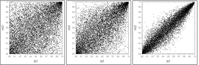
Figure 1:Rank scatter plots of the bivariate Clayton copula forθ=0.5,θ=2,θ=10.

3.1.1 The Clayton Copula

The Clayton copula, sometimes also called the Cook-Johnston copula, is defined by its generating function

φ(t) =1

θ

t−θ₋1. (17)

In the bivariate case, this leads to the cumulative copula density

C(u,v) =max

h

u−θ+v−θ₋1i−

1/θ

,0

. (18)

Scatter plots of the bivariate Clayton copula are shown for various values ofθin Fig-ure 1. It can be seen that the higher the value ofθ, the more the two random variables depend on each other. The limitθ_→0 corresponds to the uniform copula, i.e. the random variables are independent.

The Clayton copula is asymmetric. In its defined form, the Clayton copula acts on the lower tail of the distribution, whereas for upper tail the random variables are hardly dependent on each other. In insurance, however, the dependence should be modelled for the upper tails. This can easily be obtained by mirroring the copula by a transfor-mation(u,v)→(1−u,1−v). Throughout the following sections, we will consider the Clayton copula in its mirrored form.

3.1.2 The Gumbel Copula

The Gumbel copula is another representative of the family of Archimedean copulas. Its generating function is defined as

φ(t) = (−logt)θ. (19)

For the bivariate case, this leads to the cumulative copula density of

C(u,v) =exp

−h(−logu)θ+ (−logv)θi1/θ

Figure 2:Scatter plots of the bivariate Gumbel copula forθ=1.5,θ=2,θ=5.

Scatter plots of the bivariate Gumbel copula are shown for various values ofθin Fig-ure 2. As in the case of the Clayton copula, the dependence of the random variables grows with increasing value ofθ. In contrast to the Clayton copula, the Gumbel depen-dence acts on both upper and lower tail. Nevertheless, the Gumbel copula is asymmet-ric: in its definition, the dependence of high quantiles is stronger than the one of low quantiles.

3.2

Elliptical Copulas

Elliptical copulas are based on multivariate elliptical distributions, which are described for instance in [Fang and Zhang, 1990]. Prominent members of the family of elliptical copulas are the Gauss copula and the Student’s T copula. They will be described in the following subsections.

3.2.1 The Gauss Copula

The Gauss copula is the copula representation of a rank correlation process. It is based on the multivariate normal distribution. AssumingZ= (Z1, . . . ,Zn)to be a vector of

multivariate normally distributed random variables, the joint probability density func-tion is defined as

f(z) = 1 (2π)n_|Σ_|exp

−1

2z

′_Σ−1_z

, (21)

wherez= (z1, . . . ,zn)is a realisation ofZ. The correlation matrixΣis defined as

Σ= 

   

1 ρ12 . . . ρ1n

ρ21 1 . . . ρ2n

..

. ... ...

ρn1 ρn2 . . . 1



   

, (22)

whereρi jdenotes the correlation between the random variablesZiandZj. The

Figure 3:Rank scatter plot of the Gauss copula forρ=0.3,ρ=0.6, andρ=0.9.

In order to obtain the cumulative probability of the marginal distributions, i. e. the vectoruas described above, the cumulative density function of the univariate standard normal distribution has to be calculated:

ui=Φ(zi) =

1 2π

Z zi

−∞dtexp

−t 2 2 . (23)

Scatter plots of the bivariate Gauss copula are shown for various values of the correla-tion parameterρin Figure 3. The symmetry and linearity of the Gauss copula can also be seen reflected in the scatter plots: the same dependence is homogeneous for low and high quantiles, i. e. the rank correlation within any ellipsoid around the diagonal of the scatter plot is the same. The Gauss copula has become popular in stochastic simula-tion, mainly due to the simplicity of calibrating it by measuring the rank correlation. Furthermore, the algorithms of simulating multivariate random variables using a Gauss copula are well known. Nevertheless, as we will see in this article, the symmetry and the linearity of the Gauss copula are strong restrictions for modelling the dependence; assuming that in reality we observe an asymmetric dependence of insurance losses, as we argue for in the introduction, the risk diversification gain is substantially overesti-mated.

3.2.2 The Student’s T Copula

As the Gauss copula is based on the multivariate normal distribution, the Student’s T copula is based on the multivariate Student’s T distribution. A detailed discussion of the Student’s T copula can be found in [Demarta and McNeil, 2005].

LetY= (Y1, . . . ,Yn)be a random variable with a multivariate Student’s T distribution

withνdegrees of freedom. The probability density function is given by

f(y) = Γ

ν+n

2

Γ ν

2

p

(πν)n_|Σ_|

1+y′Σ−

1_y

ν

−ν+2n

. (24)

Figure 4:Rank scatter plots for Student’s T copula with constantν= 1 and increasing ρ= 0.3, 0.6 and 0.9 shown in the top row; and for constantρ=0.6 and increasingν= 1, 3 and 9 in the lower row

even more apparent when looking at the representation

Y=√WZ, (25)

whereZis a random variable with a multivariate normal distribution as described in Equation (21) andW is independent fromZand is inverse gamma distributedW _∼ Ig(ν/2,ν/2). The degree of freedom parameterνcan assume any positive real value. However, it is more difficult to find fast numerical algorithms for non-integer values of

νthan for integer values. Thus, many modellers prefer to work with integer values of

ν.

Similarly to the case of the Gauss copula, the cumulative probability of the marginal distributionsucan be obtained by calculating the cumulative distribution function of the univariate Student’s T distribution

ui=

Γ ν+1 2

Γ ν

2

√_πν

Z yi

−∞

dt

1+t

2

ν

−ν+21

. (26)

4

Setup of the Analysis and Methodology

4.1

Model Setup

In this article, we are interested in a variety of questions related to the estimation of diversification benefits when combining multiple risk factors. Foremost, we want to investigate the impact of the functional form of a copula. We will start our investigation by defining a benchmark sample that we will use as the reference to compare results.

Let us consider a standard property reinsurer whose products cover two perils: fire and windstorm. Our model reinsurer sells products in Germany and France. We will first have to think about how to set up a dependence structure for this business.

The windstorm peril underlies a strong dependence between Germany and France, as those are neighbouring countries, and the likelihood is big that a windstorm could pass over both countries in the same event. In an advanced company, the natural catastrophe peril windstorm would normally be modelled in an event set based way, which would include its dependence. However, for the sake of our investigation, we will assume that our model reinsurer has modelled the windstorm peril for both countries separately in the form of lognormal distributions and wants to model the windstorm dependence through a copula.

The fire peril underlies also a strong dependence between both countries. This may seem surprising at first glance: Why should a fire break out in Germany when there is a fire in France or vice versa? However, significant dependence between reinsurance products do not arise through the underlying peril itself but are caused by changes in legislation and insurance practice. Since both, France and Germany, are EU countries, their legislation will move somewhat in parallel. This implies a dependence between the fire losses.

Between the aggregate fire and windstorm perils, we want to model another depen-dence. The origin of this dependence is in both the reasons mentioned above: When-ever a windstorm event happens, it is likely to cause a number of fires in the correspond-ing country. Furthermore, both perils usually underlie a similar product definition and legislation and are therefore dependent. In conclusion, we model the dependence in the form of a hierarchical tree as shown in Figure 5: we subdivide the property portfolio of our model reinsurer into the perils fire and windstorm first and then into the peril regions Germany and France. This hierarchical structure is a natural way of expressing the dependence through our understanding of the business we are analysing. Moreover, there is nothing in this approach that prevents us to use an event loss set based model for windstorm to replace the lognormal model we will use throughout this article.

Figure 5:Model hierarchy used as a reference for comparing models.

probability density function (PDF) is defined as

f(x) = 1

xσ√2πexp

−(logx−µ)

2

2σ2

. (27)

We chooseµ=10 andσ=1 for each of the marginal distributions modelling our risk factors. For our purposes, the choice ofµ is hardly relevant; it is just a translational shift of the lognormal distribution and will not change our considerations on the di-versification gain. The parameterσinfluences the width and also the skewness of the distribution. The value ofσ=1 chosen for our study corresponds to a usual skewness of an aggregate insurance loss distribution.

As described in the introduction, there is strong evidence that the dependence of in-surance claims are asymmetric: Whereas it is less likely that low claim sizes in one line lead to low claim sizes in the other, it is very likely that large claims in one line trigger large claims in other lines. Therefore, we will choose the most asymmetric and the most severe one of the four copulas we investigate for our reference model to pro-duce our benchmark sample: the Clayton copula. We chooseθ=3 as the dependence between the windstorm regions,θ=2 as the dependence between the fire regions, and

θ=1 as the dependence between fire and windstorm. These parameters are higher than the ones observed in reality; the strong dependence of the reference model is chosen to strengthen the effects studied in this article and to increase the understanding. We deliberately choose an extreme case to better study the effect of dependence on the di-versification gain. We want to see how the various methods fair in reproducing a rather difficult case of dependent variables.

about aggregate losses than it is to think about copula densities.

In the following sections, we will investigate the behaviour of this reference model structure and how it can be modelled undermisspecification, i. e. using the ‘wrong’ functional form of the copula or using different hierarchies.

4.2

Methodology

The difficulty about our model setup is that many computational algorithms have to be combined to a consistent set of methods. The essential features needed are the generation of hierarchical random numbers and fitting methods for copulas. Both topics are well documented in the literature.

Algorithms to generate random variables from multivariate Archimedean copulas can be found for instance in [Whelan, 2004]. Gauss copulas are best sampled from using the methodology described by [Wang, 1998]. Student’s T copulas can be generated out of the Gauss copulas by extending Wang’s algorithm with the method described by [Demarta and McNeil, 2005].

In our study, we do not only want to generate samples from multivariate copulas, but from a hierarchical copula tree. The literature on this topic becomes sparser. Most authors follow the definition and approach as defined in [Savu and Trede, 2006]. How-ever, as mentioned above, our definition of a copula tree is slightly different: we define dependence between aggregate losses rather than between cumulative copula densities as in [Savu and Trede, 2006]. We have therefore developed a reordering schema to gen-erate hierarchical copulas, the description of which would lead beyond the scope of this article. It will be described in detail in a succeeding article [B¨urgi and M¨uller, 2008].

In the study, we define a benchmark set of observations with small theoretical diversi-fication benefits. We then fit those observations with various models of dependence. In the following paragraphs, we describe which methods we use to fit the various depen-dence model we presented in Section 3.

The fitting of Archimedean copulas was done with maximum likelihood estimation, see for instance [Savu and Trede, 2008]. GivenNvectors of observationsU1, . . . ,UN,

the log-likelihood function ofθis defined as

logL(θ) =

N

∑

j=1

logc(Uj), (28)

wherec(Uj)is the copula density ofUj. The estimator ofθis then given as the

maxi-mum of the log-likelihood function

ˆ

θ=max

θ logL(θ). (29)

The correlation matrix of the Gauss copula was determined by measuring Spearman’s rank correlation as given in Equation (3) and deriving the correlation coefficientρi jas

ρi j=2 sin

π

6RCi j

Figure 6:Value scatter (top) and rank scatter (bottom) of the reference perils.

This procedure is described in detail in [Wang, 1998].

The correlation matrix of the Student’s T copula was estimated by estimating the Kendallτi jbetween the random variablesXiandXjas given in Equation (4) and

cal-culating the correlation

ρi j=sin

π

2τi j

. (31)

The degree of freedom parameterνis estimated using maximum likelihood estimation. This method is described in more detail in [Demarta and McNeil, 2005].

5

Results and Discussion

Table 1: Parameters of the Gumbel (first row), the Gauss (second row), and the Stu-dent’s T (third row) hierarchies fitted to the Clayton reference model for fire Germany / fire France (left), fire / windstorm (middle), and windstorm France / windstorm Germany (right).

Fire Fire/Windstorm Windstorm

Gumbel θˆ=2.07 θˆ=1.54 θˆ=2.61 Gauss ρˆ=0.7 ρˆ=0.5 ρˆ=0.8 Student’s T ρˆ=0.71; ˆν=6 ρˆ=0.51; ˆν=9 ρˆ=0.81; ˆν=4

only use the rank scatter plots for the further discussions and we will call them simply scatter plots dropping the ‘rank’.

5.1

Modelling under Misspecification

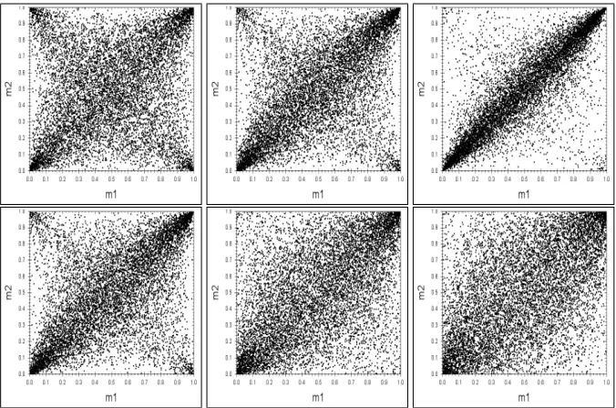
First of all, we will study the impact of the functional form for modelling dependence on the risk. For this purpose, we generate 100’000 samples from the reference struc-ture, our benchmark sample, which we will use as the realisations, i. e. the ‘observa-tions’. The other copulas described in Section 3 are fitted to those realisations, one for each node of the dependence tree.

The fitted parameters can be seen in Table 1. Since the reference hierarchy is cali-brated with a strong Clayton copula, also the fitted copula types show high values of their parameters. As a first analysis, let us look at the scatter plots in Figure 7. The Gumbel copula models the Clayton reference quite well. Due to its asymmetry, the fit of the upper tail looks optically similar. For low quantiles, the Gumbel copula models a weak dependence, whereas the Clayton implies almost independence in the lower tail. The Gauss and the Student’s hierarchies, however, deviate quite significantly from the Clayton reference. Both these copulas are symmetric, and therefore, the fits of the lower tail (striving to uncorrelated) and of the upper tail (striving to high correlation) are competing with each other. Looking at the upper tail, which is of particular impor-tance to us, we notice that the tail of the Clayton is much more pointed than the ones of the elliptic copulas. Due to its additional degree of freedom parameter, the Student’s T copulas model more points in the upper left and lower right corners of the scatter plot than the Gauss copulas.

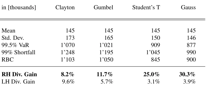
Table 2: Key statistics for the Clayton reference and the fitted hierarchies. All figures, except for the diversification gain, are in thousands.

in [thousands] Clayton Gumbel Student’s T Gauss

Mean 145 145 145 145

Std. Dev. 173 165 150 146

99.5% VaR 1’070 1’021 909 877

99% Shortfall 1’248 1’195 1’045 990

RBC 1’103 1’050 845 900

RH Div. Gain 8.2% 11.7% 25.0% 30.3%

LH Div. Gain 9.6% 5.7% 3.1% 3.9%

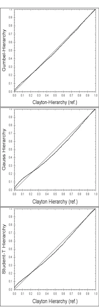
stronger correction in the upper part. It can be seen that the diagonal is approached at a higher value than in the case of the Gumbel. There are a number of more sophisti-cated goodness-of-fit methods used for copula fitting, as can be found for instance in [Savu and Trede, 2008] or [Berg, 2007]. However, as we are mostly interested in the diversification gain, we will focus on analysing the statistical properties of the fitted models.

As the distribution to measure the statistical properties and the diversification gain, we take the aggregate distribution as resulting from 250’000 simulations of the corre-sponding dependency trees. The key statistics of the Clayton reference and the fitted hierarchies can be found in Table 2. The mean of the aggregate distribution is in-dependent of the dependence as is shown in Equation (1). However, in the standard deviation it can be seen that the asymmetric Archimedean copulas show significantly more volatility than the symmetric elliptical ones.

The left handed (LH) diversification gain is shown as a measure for the effect of the dependence in the lower tail of the aggregate distribution. The LH diversification gain of 9.6% of the Clayton reference may appear surprisingly low, since the risk factors are nearly independent in the lower tail. This is due to the asymmetry of the lognormal marginal distributions: The bulk of the risk of the lognormal distribution is in the upper tail. Not surprisingly, the Gumbel (5.7%) underestimates the LH diversification gain; this corresponds to the observation we have made for the scatter plots that the Gumbel models a slight dependence in the lower tail. The symmetric elliptical copulas underestimate the LH diversification gain considerably: The Gauss (3.9%) by 60% and the Student’s T (3.1%) by almost 70%. However, the LH diversification gain is only of limited importance to us. Let us now focus on the risk in the upper tail.

underestimates the 99.5% VaR by more than 20%. The Student’s T (909’000) fits the Clayton reference slightly better than the Gauss due to its additional parameterν. However, the deviation is still more than 10%.

The picture is similar and even accentuated when considering the 99% shortfall: The Gumbel (1’195’000) approximates the Clayton reference (1’248’000) the best, the Stu-dent’s T (1’045’000) underestimates the shortfall by more than 10%, and the Gauss (990’000) shows the lowest shortfall, deviating from the reference by more than 20%. The deviations of the risk-based capital (RBC), being defined as the difference between the shortfall and the mean in Equation (9), worsen the picture even more dramatically: by subtracting the same constant of all the shortfalls, the relative deviations become higher.

The diversification gain is defined as the gain in the capital when combining all four risk factors in one company as opposed to running four companies with the risk factors in-dividually, see Equation (10). In this projection of our capital figures, a highly relevant projection for all insurance companies, the deviation becomes the worst: The Clayton reference shows a diversification gain of 8.2%. The Gumbel (11.7%) overestimates the diversification gain by over 40%, whereas the Student’s T (25%) overestimates it by over 200%, and the Gauss (30.3%) overestimates it by 270%. Using the elliptical cop-ulas to model the dependencies of the risk model would lead to a gross underestimation of the risk of this company.

To illustrate the consequences such an underestimation of the risk based capital can have, assume that our model reinsurance company has implemented an active capital management. If the company calculated its capital using the wrong functional form of the copula, it would pay back too much capital to its shareholders, up to 20% of its total risk-based capital in the case of the Gauss. If reality follows the highly asymmetric Clayton copula, the model company will need to increase its capital again when the losses need to be paid. Since this capital increase is not foreseen, the company might have to pay a high price to raise funds under financial distress.

5.2

The Effect of the Hierarchy

these reasons, the influence of the dependence structure is of high relevance. This is what we study in this subsection.

Figure 9:Portfolio modelled with a flat dependence.

We will now investigate how our model portfolio behaves if the dependence is modelled in one flat basket as shown in Figure 9 rather than the hierarchical tree as considered in the previous section. First of all, we fit a single flat Clayton copula to the hierarchical reference tree. We obtain ˆθ=1.2. We repeat the same process for a flat Gumbel and obtain ˆθ=1.55. For the Gauss and Student’s T, we allow individual correlations for each pair of risk factors, which are estimated as

ˆ

ΣG=

   

1.0 0.7 0.45 0.46 0.7 1.0 0.45 0.46 0.45 0.45 1.0 0.8 0.46 0.46 0.8 1.0

   

; ΣˆS=

   

1.0 0.71 0.45 0.46 0.71 1.0 0.45 0.46 0.45 0.45 1.0 0.81 0.46 0.46 0.81 1.0

   

. (32)

The degree of freedom parameter of the Student’s T is estimated as ˆν=10.

For the elliptical copulas, the main difference between the hierarchy and the flat struc-ture consists in the correlation between the fire and the windstorm risk factors. The reason for this is that the original Clayton reference tree models a dependence be-tween the sum of the fire and windstorm perils. The flat structure, however, assumes a correlation between the underlying risk factors, and therefore, these correlations are underestimated. Note also that the degree of freedom parameter of the Student’s T is higher than in any of the three previous nodes of the hierarchical tree. Thus, the Student’s T copula can compensate slightly for the underestimated correlations.

Looking at the scatter plots in Figure 10, we see that the flat Clayton and Gumbel have the same scatter plot for all pairs of risk factors, since we have only allowed one parameter in the model. The elliptical copulas show a similar scatter plot as shown in Figure 7 for their hierarchical variants; the differences in their parameters are rather small compared to the hierarchical case.

Table 3:Key statistics for the Clayton reference and the fitted flat baskets. All figures, except for the diversification gain, are in thousands.

in [thousands] Clayton ref. Clayton Gumbel Student’s T Gauss

Mean 145 145 145 145 145

Std. Dev. 173 173 163 151 144

99.5% VaR 1’070 1’078 1’029 902 870

99% Shortfall 1’248 1’251 1’189 1’043 978

RBC 1’103 1’106 1’044 898 832

RH Div. Gain 8.2% 7.8% 12.7% 25.4% 30.3%

LH Div. Gain 9.6% 9.14% 7.2% 3.2% 4.0%

having only one parameter, and despite the model difference of fitting the dependence to all underlying risk factors rather then the sum of fire and windstorm, and despite the obvious differences in the scatter plots, the flat Clayton model fits the hierarchical reference tree almost perfectly. The quantile / quantile plots of the other fits resemble the ones of their corresponding hierarchical variants shown in Figure 10, with slightly amplified deviations due to the poorer modelling.

The key statistics of the Clayton reference and its fitted flat structures, sampled from 250’000 simulations, are shown in Table 3. The strong similarity observed in the quan-tile / quanquan-tile plot can also be seen in the statistical figures: The flat Clayton (7.8%) models the Clayton reference extremely accurately; it even underestimates the refer-ence slightly as the only model. All other flat copulas yield slightly worse but very similar results as seen for their hierarchical counterparts shown in Table 2. All devia-tions between the flat and the hierarchical variants are below 10%.

In conclusion it can be said that the error of modelling flat structures rather than hier-archical structures does not have a strong effect on the diversification gain, even when three parameters are replaced by one as in the case of the Clayton and the Gumbel. This shows that the choice of the functional form of the copula is the key driver of the diversification gain. The asymmetry of the Archimedean copulas is the essential property which allows for accurate representation of the asymmetric reference data. Even though the flat Gauss and the flat Student’s T have more parameters than the flat Clayton and the flat Gumbel, they overestimate the diversification gain considerably.

5.3

Extending the Reference Model

mod-elled by a flat structure. In this section we extend the investigation to see under which circumstances the modelling of the hierarchical structure as opposed to a flat model matters.

First of all, we extend the model from four to eight risk factors. This increases the variety of dependencies which can be modelled. We remain with the choice of equal risk factors, all lognormal distributed withµ=10 andσ=1, as we are mostly interested in the dependence. As the reference hierarchy, we choose a three-level tree as shown in Figure 12.

The eight risk factors are grouped in four pairs, each with a separate dependence. The four aggregate distributions are grouped in two pairs with a dependence, and their two aggregate distributions underlie the top-level dependence.

We stick to the Clayton copula as the functional form of the copula of the reference model to produce a benchmark sample. In order to find out where the misspecified flat model becomes inaccurate, we investigate six different reference scenarios defined in table 4 by various combinations of the Claytonθ. The goal is to see if some combina-tions would have stronger effects than others.

Scenario 1 corresponds to a straight-forward extension of our original four risk-factor model hierarchy, assigningθ=1,2,3 to the nodes withθdecreasing towards the top level. In Scenario 2, we leave the very strong dependencies at the bottom level of the tree but relax the parameters considerably for higher aggregations. In Scenario 3 we choose generally lowerθvalues, which corresponds to a moderately dependent risk model in insurance. Scenario 4 describes a highly asymmetric situation: one half of the risk factors diversify much better than the other half of the risk factors; however, there is a strong top-level dependency. In Scenario 5, we try a ‘sandwich’ hierarchy: highθ for the bottom level, lowθfor the middle level, and highθfor the top level. Scenario 6 is the reverse of Scenario 5: Low dependency at the bottom, strong dependency in the middle, and low dependency on top.

As for the functional form of the flat, misspecified structure, we will reduce our inves-tigation to the Clayton and the Gauss copulas. For the four risk factors, we have seen

Table 4:Claytonθparameters for the six reference scenarios.

Scenarios Node 1 Node 2 Node 3 Node 4 Node 5 Node 6 Node 7

Figure 12: The hierarchical reference model setup. The eight risk factors are grouped in pairs over three hierarchy levels. Each node can be modelled with a different copula.

that the flat Clayton structure matched the hierarchical reference almost perfectly in terms of its aggregate distribution. We will investigate to which degree this similarity holds for the six scenarios described in this subsection. The Gauss copula is chosen as the one fitting the Clayton reference the worst. As for the other two copulas described in this article, the Gumbel and the Student’s T, the results would be similar as the ones of the four marginal cases: they are in between the Clayton and the Gauss, the Gumbel closer to the Clayton, and the Student’s T closer to the Gauss.

The diversification gain of the hierarchical Clayton reference model, as well as the flat Clayton and flat Gauss models, are shown for all six scenarios in Table 5. It is apparent that all the diversification gains of the flat Clayton structures are in the same range as the ones for the hierarchical reference models¡indexreference model. Most deviations are of the order of 10%. The flat structure overestimates the diversification gain in two scenarios and underestimates it in four scenarios. Nevertheless, the difference

Table 5: Diversification Gain results of the Clayton Hierarchy reference model and the fitted flat Clayton and flat Gauss models.

Reference Clayton-Flat Deviation Gauss-Flat Deviation

Scenario 1: 12.1% 14.2% 17.4% 42.4% 250.0%

Scenario 2: 32.0% 29.3% -8.4% 54.3% 69.7%

Scenario 3: 55.6% 58.8% 5.8% 68.7% 23.6%

Scenario 4: 21.5% 19.9% -7.4% 44.9% 108.8%

Scenario 5: 26.7% 21.2% -20.6% 50.5% 89.1%

Figure 13:The absolute and relative deviation between the diversification benefit of the Clayton and the Gauss for increasing dependency between two risk factors.

is more pronounced than in the simpler structure above indicating that if the structure becomes more complex the flat scenario will deviate more and more from the structure. Scenario 1, the one close to the one we have investigated for the case of four risk factors, shows one of the biggest deviations of the flat Clayton versus the reference structure: 17.4%. This is mainly due to the overall strong Clayton parameters chosen. In Scenario 3, the one with moderately dependent risk factors, the deviation between the hierarchical structure and its flat variant is only 5.8%.

As observed in all previous studies, the Gauss always overestimates the diversification gain of the reference structure in all scenarios. In Scenario 1, the deviation of 250% is similar to the one observed in the case of four risk factors. In Scenario 3, the deviation of 23.6% is still considerable. Considering the rather strong deviations, it may also be interesting to note that we have allowed for fitting 28 correlation parameters in the case of the Gauss, as opposed to the single parameter in the case of the flat Clayton. Nevertheless, the diversification gains of the flat Gauss models deviate generally more than the ones of the flat Clayton models.

hierarchical reference model would matter significantly. This can be easily seen when considering that the capital allocation in the case of a flat Clayton structure would be the overall capital divided by eight, whereas in the case of the hierarchical structure, the risk factors with the stronger dependencies would attract by far more capital. More-over, we see a tendency of increasing difference when we increase the complexity of the structure.

In the above case we have examined the effect of complexity on diversification gain but it is difficult to get a feel for how the strength of the dependence between risk factors influences the ability of the models to cope. Generally we have modelled extreme dependence between risk factors to demonstrate the significance of misspecification, however, it is important to also understand the effect for weaker dependencies between risk factors as these better reflect reality. To investigate this effect we show in Figure 13 how the diversification gain modelled by the Gauss deviates from the Clayton reference as a function of increasing dependence between two risk factors. To help relate the mathematical world of copulas to real-world situations; two risk factors are typically considered to be strongly dependent when they are modelled with a tail-dependency of 50%, which corresponds to a Claytonθ= 1. It is interesting to note that the largest absolute deviation of 15.2% of RBC between the Gauss and the Clayton occurs forθ= 1. As the dependence increases further the absolute deviation between the Gauss and the Clayton declines again as diversification gain of the Clayton tends towards zero. Forθ<1, a region that can be considered to represent tail-dependencies for most other real-world (re)insurance scenarios, there also exists a notable relative deviation that is already at 10% atθ= 0.1. The relative deviation rapidly increase as the dependence between the two risk factors grows stronger, reaching 237% atθ= 1 and 1044% atθ= 4!

We have so far demonstrated the importance of selecting the correct functional form when selecting a copula for modelling and the effect of complexity on the ability to obtain a good fit. We have also tried to relate these results to the real-world. In the following two sections we now deal with the practical aspects of fitting; convergence and error; and give some insights into how to go about deriving the correct dependence between risk factors.

5.4

Fitting Copulas: How Many Points are Needed?

One of the big problems when calibrating internal models is the estimation of depen-dence parameters. The data at hand in insurance are often sparse and it is difficult to obtain relevant samples over more than a decade or two in the best cases. It is thus important to explore what are the size of samples that are needed to reasonably fit cop-ulas. This is the last question we are going to address in this study: how many points are needed to fit the copulas? It is interesting to see if there is a systematic small sample bias for certain copula types and whether certain copulas are easier to fit than others.

1. SimulateNobservations from the reference tree,

2. Fit the corresponding structure to theNobservations,

3. Re-sample the fitted scenario with 100’000 simulations,

4. Measure the diversification gain,

5. Repeat 1. – 4. twenty times.

6. Measure the mean diversification gain and the standard deviation from the twenty calculations.

The fitting convergence plot produced according to this procedure is shown in Figure 14 for all structures.

For each point, the diversification gain plus/minus one standard deviation is drawn (top). Since it is difficult to read the error bars, the fitting errors, i.e. the standard deviation of the diversification gain measurements, are plotted separately (bottom).

The main observation of the fitting convergence plot is a confirmation of our preceding analysis: There is little difference between the hierarchical and the flat structures. The choice of the functional form is by far more important than the number of observations the copulas are fitted to.

The small sample bias seen in the plots is not significant. Not surprisingly, the di-versification gain is slightly overestimated for a small number of observations, as not sufficient extreme events are used for the fits. Nevertheless, the error bars are suffi-ciently large to include the value of the diversification gain as fitted for a high number of observations. When fitting the structures to 100 observations, the small sample bias can be hardly seen in the average estimates.

In order to have a better understanding of the fitting error, let us analyse the bottom chart of Figure 14. All errors decrease significantly when moving from 20 to 100 observations. There is still a considerable drop of the errors when moving from 100 to 500 observations, whereas the errors remain rather stable for higher numbers of observations. It is interesting to note that the hierarchical Archimedean copulas have significantly higher errors for a low number of observations than their flat variants. This can be explained by the flat structures considering all observation points for fitting one parameters, whereas the parameters of the hierarchical structures are fitted each on a subset of the observation. These differences, however, vanish when moving to 100 and to 500 observations.

Figure 14: Fitting convergence plot (top) for the hierarchical and flat copula models. The mean diversification gain_±one standard deviation is shown as a function of the number of samples. The errors are shown separately (bottom).

more points in the lower tail to low correlation. The asymmetric Archimedean copulas can absorb a shift in the number of lower and upper tail points better, since they can account for the asymmetry.

Figure 15:Example of an event set based wind model.

6

Estimating Dependence

When considering the hundreds of observations needed to fit the dependence of 4 risk factors, in reality this would mean collecting (aggregate) loss experience during hun-dreds of years. Even if we could wait to collect the observations needed, it would be questionable what the significance of the fitted model is; the definitions and be-haviour of insurance products would change significantly over this period of time, and the assumption that these observations underlie the same model would not be valid. Therefore, alternative ways of modelling dependence have to be sought.

An elegant means of modelling dependence is to use an explicit physical model when-ever one is known. This is the case, for instance, for natural hazards. The contemporary models are event loss set based, i. e. the single wind, earthquake, or flood events are modelled together with a frequency of their occurrence. Given these events, the whole portfolio of risks can be evaluated yielding the aggregate loss by event. Figure 15 il-lustrates an example of an event set based wind model. Individual risk factors can be considered by describing the vulnerability of the buildings, their insured value, as well as their insurance conditions. By aggregating over all events, the dependence of the risks is implicitly reflected.

The example of the natural catastrophe perils is the most prominent and most advanced one in terms of modelling. However, many (re)insurance companies have started con-structing similar individual risk or scenario models, for instance for pricing auto liabil-ity policies. There is still a significant potential to establish further individual risk and scenario based models for insurance products.

Table 6:Relationship between the tail dependence and theθ-parameter for Clayton and Gumbel copulas.

Tail dep. 1% 2% 5% 10% 20% 30% 40% 50% 60%

Claytonθ 0.15 0.18 0.23 0.30 0.43 0.58 0.76 1.00 1.36 Gumbelθ 1.01 1.02 1.04 1.08 1.18 1.31 1.48 1.71 2.06

estimated. The form of the hierarchical tree is fairly comfortable in its usage, as there is an intuitive meaning associated with each node.

Since the copula parameters often lack an intuitive interpretation, considerations can be made about thetail dependenceof the lines aggregated in each node. Theuppertail dependenceλUandlowertail dependenceλLof a bivariate distribution are defined as

λU = lim

q→1P(X2>F

−1

2 (q)|X1>F− 1

1 (q)), (33)

λL = lim

q_→0P(X2<F

−1

2 (q)|X1<F1−1(q)). (34)

Detailed discussion on tail dependence can be found in [Embrechts et al., 2003]. It can be shown that the tail dependence is a property of the bivariate copula only:

λU = lim

q_→1(1−2u+C(u,u))/(1−u), (35)

λL = lim

q_→0(2u−1+C(u,u))/u. (36)

The idea behind the tail dependence is to ask the question with which probability a line of business has an extreme loss given that another line of business has an extreme loss. The answer to this question can be given by thinking about adverse scenarios in the portfolio. In this context, it might be especially interesting to investigate the causal relations between the individual risk factors. Interviews with the risk specialists regard-ing quantitative impact of adverse scenarios can help understandregard-ing extreme scenarios and their dependence. This is stress testing by analysing possible outcomes of extreme scenarios.

The relationship between the tail dependence and the copula parameters can be found by evaluating Equations (35) and (36) for the given copula. For the Gauss copula, it can be found that the tail dependence does not exist: the dependence implied by the rank correlation is not strong enough to yield a valueλU>0. For the Clayton and Gumbel

copulas, however, the tail dependence does exist, and the parameters can be associated with it as follows:

θClayton = −

log 2

logλ, (37)

θGumbel =

log 2

Table 6 shows a range of values of the tail dependence and the corresponding Clayton and Gumbelθvalues.

As an example, consider a product which is highly dependent on the legislation and court practice, such as a professional liability product. Two legal entities within the European Union write substantial volumes of this product in two different countries. The specialists define an extreme scenario in which a change in legislation would cause an extreme loss in the one of the countries. Since all the EU countries will develop their legislation somewhat in parallel, the specialists estimate that – given the legislation is changed in one country – the legislation would be changed in the other country with a probability of 50%. If the risk modeller decides to use a Clayton copula to model the dependence, the choice of the parameter would be aroundθ=1.

7

Conclusions

In this article, we have analysed the impact of the functional form of a copula and the hierarchical dependence structure on the risk-based capital and on the diversification gain of a portfolio of risks, which is characterized by a strong dependence in the ex-treme cases. This is a typical situation in insurance and as we have experienced it in financial markets.

The main conclusion to be drawn is that the functional form of the copula chosen for modelling has a significant impact on the diversification gain: Given an asymmetric Clayton reference model (diversification gain of 8.2%), the use of symmetric copu-las grossly overestimate the diversification gain (diversification gain of over 30% in the case of the Gauss copula overestimating the ‘true’ diversification gain by 270%). Even though the fitted parameters of the symmetric Gauss and Student’s T copulas are perceived as rather conservative, they do not manage to compensate for the symmetry effects and their lack of tail dependence in the shortfall. The Gumbel copula, which models a slight dependence in the lower tail, still yields a fairly accurate diversification gain, as it can deal better with the asymmetry of the reference model.

The impact of the hierarchy is less severe than the choice of the functional form. By reducing the hierarchical structure of the reference model to one flat node, the result-ing diversification gain is slightly higher than in the case of the hierarchical variants in most cases. The only structure which slightly underestimates the diversification gain is the flat Clayton structure, which manages to model the aggregate distribution almost perfectly. In general, the asymmetric Archimedean copulas model the reference struc-ture more accurately than the symmetric elliptical copulas even if they are reduced to a single parameter, whereas many parameters are allowed for the elliptical copulas (three and four in the case of four risk factors, 28 and 29 in the case of eight risk factors). The functional form of the copula is the decisive choice and by far more important than the dependence structure.

-100% of the reference diversification gain. The error drops considerably to around 20% - 30% of the reference diversification gain when fitting to hundreds of observations, which provides a reasonable basis for fitting dependence of four risk factors.

The conclusions of these observations are to be taken with care; let us bear in mind that a book of business is often subdivided in significantly more than four risk factors. Furthermore, we have only looked at the convergence of the overall diversification gain. As soon as partial results are in the focus of interest, for instance the capital allocation by risk factor, the detailed dependence structure of the risk model matters. Also the convergence behaviour of the fits will be slower. Therefore, the number of observations needed to fit the dependence of an entire risk model would increase. Thus a hierarchical structure, which focuses on few dependencies, is well suited to calibrate the internal model.

In practice, it is hardly possible to fit copulas for insurance risks based on historical observations. Alternatives have to be sought for estimating dependence. For some of the insurance products, it is possible to create explicit physical models which implicitly contain their dependence structure. This is an elegant alternative to using copulas. However, if no physical models can be found, the modelling with copulas is a good option.

The tail dependence is an intuitive quantity relating probabilities as defined in extreme scenarios with copula parameters. The modelling of scenarios is often easier for risk specialists than the modelling of statistical properties. Since the Gauss copula, i. e. the rank correlation, does not have tail dependence, this approach cannot be used. How-ever, when using Clayton or Gumbel copulas, easy relationships between the tail de-pendence and the copulaθcan be found, and the extreme scenarios can be used to calibrate the copulas. So much for stress testing!

References

[Acerbi and Tasche, 2002] Acerbi, C. and Tasche, D. (2002). On the coherence of expected shorfall.Journal of Banking & Finance, 26(7):1487–1503.

[Armstrong, 2003] Armstrong, M. (2003). Copula catalogue, part 1: Bi-variate Archimedean copulas. http://www.cerna.ensmp.fr/Documents/

MA-CopulaCatalogue.pdf.

[Artzner et al., 1999] Artzner, P., Delbaen, F., Eber, J.-M., and Heath, D. (1999). Co-herent risk measures.Mathematical Finance, 9:203–228.

[Berg, 2007] Berg, D. (2007). Copula goodness-of-fit testing: an overview and power comparison. Statistical Research Report, University of Oslo.

[B¨urgi and M¨uller, 2008] B¨urgi, R. and M¨uller, U. (2008). Aggregating risks in hier-archical copula trees.To be published.

[Embrechts et al., 2003] Embrechts, P., Lindskog, F., and McNeil, A. (2003). Hand-book of Heavy Tailed Distributions in Finance, chapter Modelling Dependence with Copulas and Applications to Risk Management. Elsevier.

[Embrechts et al., 2002] Embrechts, P., McNeil, A., and Straumann, D. (2002). Risk Management: Value at Risk and Beyond, chapter Correlation and Dependence in Risk Management: Properties and Pitfalls. Cambridge University Press.

[Fang and Zhang, 1990] Fang, K. T. and Zhang, Y. T. (1990). Generalized Multivari-ate Analysis. Springer.

[Genest and Favre, 2007] Genest, C. and Favre, A.-C. (2007). Everything you always wanted to know about copula modeling but were afraid to ask.Journal of Hydrologic Engineering, pages 347–368.

[Nelsen, 1999] Nelsen, R. B. (1999).An Introduction to Copulas. Springer.

[Savu and Trede, 2006] Savu, C. and Trede, M. (2006). Hierarchical Archimedean copulas. http://www.uni-konstanz.de/micfinma/conference/Files/

papers/Savu_Trede.pdf.

[Savu and Trede, 2008] Savu, C. and Trede, M. (2008). Goodness-of-fit tests for para-metric families of Archimedean copulas. Quantitative Finance, 8(2):109–116.

[Sklar, 1958] Sklar, A. (1958). Fonctions de r´epartition `a n dimensions et leurs marges. Publications de l’Institut de Statistique de L’Universit´e de Paris, 8:229–231.

[Tasche, 2002] Tasche, D. (2002). Expected shortfall and beyond.Journal of Banking & Finance, 26(7):1519–1533.

[Wang, 1998] Wang, S. S. (1998). Aggregation of correlated risk portfolios: Models and algorithms.Proceedings of the Casualty Actuarial Society, pages 848–939.

Index

calibration, 19 copula, 5

Archimedean copulas, 6 Clayton copula, 7 Gumbel copula, 7 elliptical copulas, 8

Gauss copula, 8 Student’s T copula, 9 correlation

Kendallτ, 4 linear correlation, 3 Pearson correlation, 3

Spearman’s rank correlation, 4

degrees of freedom, 9

fit

log-likelihood function, 13 maximum likelihood estimation, 13

hierarchical tree, 11

lognormal distribution, 11

reference model, 12–16, 24–26 Risk, 4

risk measure, 4

coherent risk measure, 4 expected shortfall, 5 tail-value-at-risk, 5 value-at-risk, 4 risk-based capital, 5, 32

Dr Roland B ¨urgi is a senior risk consultant in Group Financial and Risk Modelling at SCOR. His current role is as business architect of Asset and Liability Man-agement Programme, a project portfolio with the scope of implementing an in-tegrated quantitative risk management in SCOR Group. Before joining Con-verium, which later became SCOR Roland B¨urgi has worked on the pricing methodology at Swiss Re, where he has led and successfully completed sev-eral large-scale pricing projects for property and casualty business. He holds a MSc in theoretical physics from the University of Berne and a PhD in physical chemistry from the ETH Zurich.

Dr Michel M. Dacorogna , member of the senior management of SCOR, is currently

heading its Group Financial Analysis and Risk Modeling team. His main re-sponsibilities are: develop the Asset and Liability Management models for the SCOR group, assist customers in determining the best reinsurance structure tak-ing into account the full portfolio of asset and liabilities. Besides his main tasks, he actively participates in customers’ contacts and in the design of complicated contracts implying risk transfer to financial markets. He also conducts research in the field of insurance and reinsurance: capital allocation to risk, pricing and optimizing reinsurance covers, optimal asset allocation of investments, evalua-tion of credit risk, risk management of investments, forecasting models of long term economic trends. The author of more than 60 publications in refereed sci-entific journals, he often presents his results in international conferences and specialized seminars. He received his Habilitation, PhD and MSc in Theoretical Physics from the University of Geneva in Switzerland.