Exact and Efficient Bayesian Inference for Multiple Changepoint problems
Paul Fearnhead
Department of Mathematics and Statistics Lancaster University
SummaryWe demonstrate how to perform direct simulation from the posterior distri-bution of a class of multiple changepoint models where the number of changepoints is unknown. The class of models assumes independence between the posterior distribution of the parameters associated with segments of data between successive changepoints. This approach is based on the use of recursions, and is related to work on product partition models. The computational complexity of the approach is quadratic in the number of observations, but an approximate version, which introduces negligible error, and whose computational cost is roughly linear in the number of observations, is also possible. Our approach can be useful, for example within an MCMC algorithm, even when the independence assumptions do not hold. We demonstrate our approach on well-log data. Our method can cope with a range of models for this data, and exact simulation from the posterior distribution is possible in a matter of minutes.
Keywords Bayes factor, Forward-backward algorithm, Model choice, Perfect simula-tion, Reversible jump MCMC, Well-log data
1
Introduction
Many time-series models incorporate one, or multiple, changepoints. Some examples include Poisson processes with a piece-wise constant rate parameter (Raftery and Ak-man, 1986; Yang and Kuo, 2001; Ritov et al., 2002), changing linear regression models (Carlinet al., 1992; Lund and Reeves, 2002), Gaussian observations with varying mean (Worsley, 1979) or variance (Chen and Gupta, 1997; Johnsonet al., 2003), and Markov models with time-varying transition matrices (Braun and Muller, 1998). Such models have been used for modelling stock prices, muscle activation, climatic time-series, DNA sequences and neuronal activity in the brain, amongst many other applications
models assumes that the parameter values associated with each segment are independent from each other. Yang and Kuo (2001) comment that calculating the Bayes factors for models with different numbers of changepoints is “essentially infeasible for a large model with many changepoints”. Our aim is to show that calculation of Bayes factors, and perfect sampling from the posterior distribution of changepoint locations, is both possible, and computationally inexpensive for the class of models we consider. While this class of models may seem restrictive, recent examples of work on such models can found in Johnsonet al. (2003), Punskayaet al. (2002), and Braunet al. (2000). Although we use the phrase “perfect simulation”, we do not use coupling-from-the past (Propp and Wilson, 1996), or related ideas, which have become synonymous with this phrase. Instead, the work we present is closely related to work by Yao (1984), Barry and Hartigan (1992) and Barry and Hartigan (1993). These papers present efficient recursions that allow the posterior probabilities of different numbers of changepoints, and the posterior mean of the parameters to be calculated. Despite the desirability of exact solutions, and the simplicity and computational efficiency of the recursions, these methods are currently underused. We extend these methods to allow for direct simu-lation from the posterior distribution of the number and position of the changepoints, and to also perform inference conditional on the number of changepoints.
Much recent research for changepoint models is based on the use of MCMC. For models with an unknown number of changepoints, a common approach is that of Green (1995). A set of models, each incorporating a different number of changepoints, are introduced, and reversible jump MCMC is used to explore the joint space of model and parameters. Potential difficulties of this approach include designing moves, particular ones between different models, which enable the MCMC algorithm to mix well (for guidelines on de-signing reversible jump MCMC algorithms see Brooks et al., 2003), and being able to detect convergence of the algorithm. For example, in the analysis of the coal-mining disaster data in Green (1995), the reversible jump MCMC algorithm had not converged. The reanalysis of the data in Green (2003), using a reversible jump MCMC algorithm run for 25 times as long, does fully explore the posterior distribution. The exact simu-lation method we describe here avoids any problems of needing to diagnose convergence of an MCMC algorithm.
position. The other is based on modelling the changepoint process by a point process (Pievatolo and Green, 1998), and is a special case of a product-partion model (Hartigan, 1990). This indirectly specifies a joint prior on the number and position of the change-points. In both cases we assume that, conditional on the realisation of the changepoint process, the joint posterior distribution of the parameters is independent across the segments of the time series. We also assume a conjugate prior for the parameters asso-ciated with each segment. Under these two assumptions we derive a set of recursions to perform exact inference.
The recursions are similar to those of the Forward-Backward algorithm (see Scott, 2002, for a review). Recent work has shown how such recursions can be used to perform exact inference for a range of problems (Fearnhead and Meligkotsidou, 2004; Fearnhead, 2004). The assumption of independence between segments ensures the necessary Markov prop-erty that is required for Forward-Backward type recursions. For a data set consisting of observations at discrete times, 1, . . . , n, the recursions are based on calculating the probability of the data from time tto time n, given a changepoint at time t, in terms of the equivalent probabilities at timest+ 1, . . . , n. Once these probabilities have been calculated for all time-points, it is possible to directly simulate from the posterior dis-tribution of the time of the first changepoint, and then the conditional disdis-tribution of the time of the second changepoint, given the first, and so on. The recursions can also be used to perform exact inference conditional on the number of changepoints, and in some cases to calculate the posterior distribution of the parameters that govern the point process model for the changepoints.
The outline of the paper is as follows. In Section 2 we introduce the two classes of changepoint model that we consider. The recursions are derived and detailed in Section 3. The resulting algorithm is demonstrated on well-log data in Section 4. We consider a range of models for this data, and also demonstrate how our method can be used to analyse the data when there is dependence between the parameters for each segment. The paper concludes with a discussion.
2
Models and Notation
We consider the following class of multiple changepoint models. Consider a sample of size n, y1, . . . , yn. Observation yi is obtained at time i, and we let yi:j denote the observations from timei to timej inclusive.
Firstly condition onm integer-valued changepoints, at points 0< τ1< τ2 <· · ·< τm<
n. We letτ0= 0 and τm+1=n. Then thejth segment consists of the observations from
time τj−1+ 1 to time τj. We associate a (possibly vector-valued) parameter θj with
thejth segment forj= 1, . . . , m+ 1. Conditional on the change-points and parameter values, the observations are independent; observation yi being drawn from a density
f(yi|θj) if timeiis in the jth segment.
We assume independent priors for the parameters associated with each segment. The prior for θj is denoted by π(θj). Here, and throughout, we useπ(·) solely to denote a prior density; the argument making it clear as to which parameter the prior is for. We assume that the changepoints occur at discrete time points, and consider two priors for the changepoints. The first prior is based on a prior for the number of changepoints, and then a conditional prior on their positions. We will define this conditional prior on the positions in terms of πm(τm) the prior for the last change point, and, for j = 1, . . . , m−1, πm(τj|τj+1), the prior for the position of the jth changepoint, given the
position of the (j+ 1)st.
If G(t) =Pts=1g(s), is the distribution function of the distance between two succesive points, andg0(t) is the mass function of the first point after 0, then the probability of m changepoints occuring at τ1, . . . , τm is
g0(τ1)
m Y
j=2
g(τj−τj−1)
(1−G(τm+1−τm)).
Natural choices for the distribution of the time between successive points are from the negative binomial family. For a negative binomial distribution with parameters k, a positive integer, andp we have
g(t) =
t−k
k−1
pk(1−p)t−k g0(t) = k X
i=1
t−i
i−1
pi(1−p)t−i/k.
The negative binomial distribution can be thought of as a discrete version of the gamma distribution (especially if p is small). If k= 1 then the negative binomial distribution is the geometric distribution, and the point process is Markov. Larger values of k can reduce the number of very short segments.
3
Filtering Recursions
We first derive the recursions for analysing data under the point process prior for the changepoints. We later derive recursions to perform inference conditional on the number of changepoints, and show how these can be used to perform inference under the other prior, and to perform inference about the parameters of the point process prior.
3.1 Basic Recursions
For times s≥t, define
P(t, s) = Pr(yt:s|t, sin the same segment) =
Z s Y
i=t
f(yi|θ)π(θ)dθ.
We will assume that the probabilities P(t, s) can be calculated for all t and s. In practice this will require conjugate priors on θ, or, if θ is low-dimensional, that the required integration can be calculated numerically.
We next define fort= 2, . . . , n
with Q(1) = Pr(y1:n). A set of recursions for calculating these probabilities are given
by the following theorem.
Theorem 1 Define the probabilities Q(t) and P(t, s) as above. Then for t= 2, . . . , n
Q(t) = n−1
X
s=t
P(t, s)Q(s+ 1)g(s+ 1−t) +P(t, n)(1−G(n−t)), (1)
and
Q(1) = n−1
X
s=1
P(1, s)Q(s+ 1)g0(s) +P(1, n)(1−G0(n−1)), (2)
where G0(t) =Pts=1g0(s).
Proof: We only prove Equation 1. Equation 2 can be derived similarly.
For notational convenience we drop the explicit conditioning on a changepoint att−1 in the following. Thus,
Q(t) = Pr(yt:n) =
n−1
X
s=t
Pr(yt:n,next changepoint ats) + Pr(yt:n,no further changepoints).
Now these probabilities can be calculated by the product of the prior probability on the changepoints, and the probabilities of the observations from a single segment, P(t, s). Thus
Pr(yt:n,next changepoint at s)
= Pr(next changepoint at s) Pr(yt:s, ys+1:n|next changepoint ats) = g(s+ 1−t) Pr(yt:s|t, s in same segment) Pr(ys+1:n|changepoint ats)
= g(s+ 1−t)P(t, s)Q(s+ 1)
Similarly
Pr(yt:n,no further changepoints) =P(t, n)(1−G0(n−t)),
as required. 2
Equations 1 and 2 give recursions that can be used to calculate Q(t) in turn for t =
The computational complexity of the resulting algorithm is quadratic in n. However often only a small proportion of the terms on the right-hand side of (1) make an ap-preciable contribution toQ(t). This can happen when the data makes it almost certain that a changepoint occurs before a given time-point. Thus the summation can often be truncated with negligible error. We propose truncating the sum at term k when
P(t, k)Q(s+ 1)g(k+ 1−t) Pk
s=tP(t, s)Q(s+ 1)g(s+ 1−t)
(3)
is less than some predetermined value, for example 10−10.
In the limiting regime of analysing a process over a longer time period, so that the number of changepoints will increase roughly linearly with the number of observations,
n, the computational complexity of the resulting approximate set of recursions will be linear in n. Essentially the average number of terms required in the right-hand side of (1) will be constant with t. Thus the average computational cost of one of the n
recursions will be independent ofn.
3.2 Perfect Simulation of Changepoints
Given the values of Q(t) for t = 1, . . . , n it is straightforward to simulate from the posterior distribution of the changepoints as follows.
The posterior distribution of the first changepoint is given by
Pr(τ1|y1:n) = Pr(y1:n, τ1)/Pr(y1:n)
= Pr(τ1) Pr(y1:τ1|τ1) Pr(yτ1+1:n|τ1)/Q(1)
= P(1, τ1)Q(τ1+ 1)g0(τ1)/Q(1),
forτ1 = 1, . . . , n−1. The probability of no further changepoint beingP(1, n)(1−G0(n−
1))/Q(1).
Similarly the posterior distribution of the τj given τj−1 is
Pr(τj|τj−1, y1:n) =P(τj−1+ 1, τj)Q(τj + 1)g(τj −τj−1)/Q(τj−1+ 1),
for τj = τj−1+ 1, . . . , n−1, and the probability of no further breakpoint is P(τj−1+
1, n)(1−G0(n−τj−1−1))/Q(τj−1+ 1).
denote the generic posterior distribution of the next changepoint, given a changepoint at t by Pr(τ|y1:n, t), which can be calculated as above.
(1) For a sample of size M, initiate each of the M samples with a changepoint at
t= 0.
(2) Fort= 0, . . . , n−2:
(i) Calculatentthe number of whose last changepoint was at time t. (ii) If nt>0 calculate the probability distribution Pr(τ|y1:n, t).
(iii) Sample nt times from Pr(τ|y1:n, t) using Algorithm 1 of Carpenter et al. (1999) (see the Appendix). Use these values to update the nt samples of changepoints which have a changepoint att.
There are two advantages of this algorithm. The first is that the probability mass function Pr(τ|y1:n, t) need only be calculated once regardless of the number of samples required from it. If changepoints are sampled one at a time, then either these densities will, potentially, need to be calculated for each sample, or they will need to be stored. Storing these mass functions can place large burdens on computational memory. The storage requirements will be quadratic in n; by comparison the above algorithm has storage requirements that are linear inn.
The second is that simulating a sample of sizem from a general discrete mass function can be achieved more efficiently than sampling m samples of size 1. Algorithm 1 of Carpenter et al. (1999) allows a sample of size m to be simulated with order n+m
effort, rather than the nmeffort of samplingm samples of size 1.
3.3 Conditioning on the Number of Changepoints
Now consider inference conditional on m changepoints. As in Section 2 we define the prior for the changepoints viaπm(τm) and conditional probabilities of the formπm(τ+
j|τj+1). We defineP(s, t) as before, and forj= 1, . . . , m, andt=j+1, . . . , n−m−1+j,
Q(jm)(t) = Pr(yt:n|τj =t−1, m changepoints).
We can derive the following set of recursions. Fort=m+ 1, . . . , n−1,
Forj = 1, . . . , m−1, andt=j+ 1, . . . , n−m−1 +j
Q(jm)(t) = n−m+j
X
s=t
P(t, s)Q(jm+1)(s+ 1)πm(τj =t−1|τj+1 =s).
Finally
Pr(y1:n|m changepoints) =
n−m
X
s=1
P(1, s)Q(1m)(s+ 1). (4) These can be proved in a similar way to Theorem 1.
If the number of changepoints is unknown, with prior π(m), then the posterior distri-bution of mcan be calculated as
Pr(m|y1:n)∝π(m) Pr(y1:n|m changepoints),
with the last term, the evidence formchangepoints, being calculated, for eachm, using the recursions.
Simulation from the joint posterior distribution is possible by first simulatingMsamples from Pr(m|y1:n). If the value m is sampled Nm times, then Nm samples from the posterior distribution of the changepoint positions, conditional onmchangepoints, can be obtained as described in Section 3.2. The only difference is that the conditional distribution of τj given τj−1 is now
Pr(τj|τj−1, y1:n, m) =P(τj−1+ 1, τj)Q
(m)
j (τj+ 1)πm(τj−1|τj)/Q
(m)
j−1(τj−1).
Finally, in the case of the Markov point process prior (that is, a geometric distribution for the distance between changepoints), exact inference is possible even if the probability of a changepoint at any timepoint, p, is unknown. This is because, conditional on the number of changepoints, the positions are distributed uniformly along the interval, independent of p. We can thus perform inference conditional on m changepoints. The prior form is obtained by averaging π(m|p) with respect to the prior for p.
4
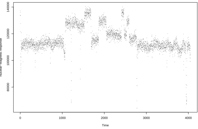
Well-log Data
0 1000 2000 3000 4000
80000
100000
120000
140000
Time
[image:10.595.134.482.88.314.2]Nuclear−Magnetic response
Figure 1: The well-log data.
were taken at discrete timepoints by the probe as it was lowered through the hole. The underlying signal is roughly piecewise constant, with each constant segment relates to a single rock type (that has constant physical properties). The changepoints in the signal occur each time a new rock type is encountered. Detecting the changepoints is important in oil-drilling; see the introduction of Fearnhead and Clifford (2003) for more details.
These data have been previously analysed by ´O Ruanaidh and Fitzgerald (1996), who used MCMC to fit a change-point model with a fixed number of changepoints; and by Fearnhead and Clifford (2003) who considered online analysis of the data using particle filters. We performed a batch analysis of the data, but allowed for multiple changepoints.
4.1 Piecewise constant model
Initially we consider analyse based on a model taken Fearnhead and Clifford (2003). We assume a Markov point process prior, with p= 1/250, for the changepoints. There are a number of outliers in the data which were removed before the data was analysed. For a timet which belongs to segment i, we model a non-outlying observation, yt, by
36 38 40 42 44 46 48 50 52
(a)
Number of Changepoints
Posterior Probability
0.00
0.05
0.10
0.15
(b)
Time
Probability
0 1000 2000 3000 4000
0
1
0 1000 2000 3000 4000
100000
120000
140000
(c)
Time
Nuclear Response
0 1000 2000 3000 4000
100000
120000
140000
(d)
Time
[image:11.595.107.510.90.370.2]Nuclear Response
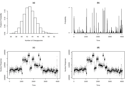
Figure 2: Results of analysis of the well-log data. Figures (a)–(c) are a model with
p = 0.004: histogram of number of changepoints(a); posterior distribution of position of changepoints (b); and 20 simulations from the posterior distribution of the signal (c). Figure (d) shows 20 simulations from the posterior distribution of the signal when
p= 0.013.
whereµiis the mean associated with theith segment, and we assume a common known variance, σ2 = 25002. We assume that the segment means have independent normal priors with mean 115,000 and variance 10,0002. Conditional on the segment means, the observations are independent.
The results of our analysis are shown in Figure 2(a)–(c). These plots are for the pos-terior distribution of the number of changepoints and their positions (based on 10,000 independent simulations from the posterior), and 20 realisations of the underlying sig-nal. It took 26 seconds on a 3.4GHz PC to perform this analysis. The results we obtain differ substantially from previous analyses. The posterior distribution suggests around 40 changepoints, which is roughly three times as many as assumed by ´O Ruanaidh and Fitzgerald (1996). Fearnhead and Clifford (2003) only infer 16 changepoints. However theirs is an online analysis, so inference at each timepoint is based solely on the ob-servations to that timepoint. Furthermore, they only inferred a changepoint when the posterior probability of changepoint within the last 10 time-points was greater then 0.9. This is likely to produce a conservative estimate of the number of changepoints. The posterior mean of the number of changepoints, 43, is much larger than the 8 to 26 changepoints we would expect under our prior. Using the methods of Section 3.3 we can perform inference whenpis unknown. If we assume a uniform prior forp, then the posterior mode is at p= 0.013. Some results of analysing the data with this value ofp
are shown in Figure 2(d). The posterior distribution for the number of changepoints is substantially different, with a posterior mean of 52 (not shown), but realisations from the posterior distributions of the underlying signal are similar to those whenp= 0.004. We repeated our analysis using the approximate algorithm suggested in Section 3.1. We truncated the sums in Equations (1) and (2), used to calculate theQ(t)s, when the value of (3) was less than 10−10. The resulting algorithm on average required sums of 222
terms to be calculated for each Q(t); which compares with average sums of 2025 terms for the exact algorithm. This is nine-fold reduction in the complexity of the algorithm. The resulting approximation of the log evidence was correct to 4 decimal places, which suggests that negligible errors were introduced.
4.2 Inclusion of Hyperpriors
We now consider an extension of the above model where all parameters in our model were unknown, and we introduce hyperiors for them. This introduces dependence between the segments, and our direct simulation algorithm has to be used with an MCMC scheme,
parame-terised the prior for the segment means as
µi ∼N(η, τ2σ2),
and used improper hyperpriors on η and τ: π(η)∝1 andπ(τ)∝1/τ.
We analysed this model using MCMC. The MCMC algorithm used the following three updates:
(1) Update the changepoints conditional onσ,p,η, and τ. We used an independent proposal from the true posterior distribution conditional onσ = 2,330,p= 0.013,
η= 115000, andτ = 4.3.
(2) Updateσ,pand theµis from their full conditional distribution given the change-points andη and τ.
(3) Updateη andτ from their full-conditionals given theµis.
Each of these moves satisfies detailed balance. Steps (2) and (3) are Gibbs steps, and thus the proposed values are always accepted. Step (1) is not a Gibbs step. Although it would be possible to make it so, there is a substantial overhead to calculating the posterior distribution of the changepoints at each iteration. Thus while this algorithm may mix more slowly, a single iteration will be substantially quicker, and hence we hope it will be more efficient. In updating the changepoints in step (1) we throw away the segment means. This is an example of collapsing (Liu, 2001, pages 146–151 ), which usually improves the mixing of the Markov Chain.
We ran this Markov chain for 10,000 iterations. The acceptance probability of step (1) was 61.8%. The 1-lag autocorrelation for each of the parameters was less than 0.03, which suggests that the chain is mixing extremely quickly.
4.3 Alternative Models
The models used in the previous Sections are based around those previously used in the literature for this data. However the realisations from the posterior distribution have many more changepoints, and thus suggest many more rock strata, than is realistic. It appears that the piecewise constant model used is overly simplistic for the data, and that this has resulted in the need for too many changepoints in order to fit the data. We have considered numerous extensions to the model. Two possibilities are: (i) to allow different noise variances for different segments; and (ii) to model each segment using a mean-shifted AR(1) model (Albert and Chib, 1993). Both of these models can be analysed via our direct simulation method, though for (ii) we need to numerically integrate out the autoregressive coefficient (this can be done in a similar way to that described below). However neither of these extensions enable the data to be fit with substantially fewer change points (results not shown).
Instead we consider the following state-space model for the data within a segment, where if t−1 and tboth lie within segment i
µt ∼ N(µt−1, τ
2
i)
yt ∼ N(µt, σ2).
The initialµvalue for each segment is drawn from the same independent normal priors as before. This is an extension of the piecewise constant model which allows the signal within a segment to perform a random walk. We allow the variance of the random walk to vary among segments, and assume a Gamma prior forτiwith parameters 2 and 1/40. This prior places most probability mass on values ofτi which lie in the interval [0,150]. The idea of this model is that the random walk element can fit the small-scale variation in the underlying signal without the need to infer changepoints.
Ifτi were known for each segment then it would be straightforward to apply our direct simulation method, using the Kalman Filter (Harvey, 1989) to integrate out the under-lying signal. To incorporate a prior onτi we resort to numerical integration to calculate the P(t, s) values required by our algorithm. A simple, but adequate, approach to nu-merical integration is based on using a grid ofτi values, and we obtained such a grid as follows. For a grid with K points, first simulate for k = 1, . . . , K, a realisation, uk, of a uniform random variable on [(k−1)/K, k/K]; then fix the kth grid point to be the
12 14 16 18 20 22 24 26 28
(a)
Number of Changepoints
Posterior Probability
0.00
0.05
0.10
0.15
(b)
Time
Probability
0 1000 2000 3000 4000
0
1
0 1000 2000 3000 4000
100000
120000
140000
(c)
Time
Nuclear Response
0 1000 2000 3000 4000
100000
120000
140000
(d)
Time
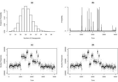
[image:15.595.107.509.90.370.2]Nuclear Response
Figure 3: Results of analysis of the well-log data. using the state-space model: histogram of number of changepoints(a); posterior distribution of position of changepoints (b); and realisations from the posterior distribution of the signal (c)–(d). The results for (a) and (b) are based on 10,000 perfect simulations from the posterior distributions.
In practice we found that a grid of 100 points produced accurate results; and for such a grid it took less than 19 minutes to simulate 10,000 draws from the joint posterior distribution of changepoint positions on a 3.4GHz PC. The results of the analysis (as-sumingσ = 2,500 andp= 0.004) are shown in Figure 3. This model gives more realistic inferences about the number and positions of the changepoints. Further refinements of the model may be appropriate and could further improve the inferences, for example by choosing a distribution for the segment lengths that does not allow very short segments, but these are not considered here.
5
Discussion
men-tioned previously, the work we present is closely related to work by Barry and Hartigan (1992). The main novelty of what we propose is that we demonstrate how the recur-sions can be used for perfect simulation from the posterior distribution of the number and position of change-points, and hence from the posterior distribution of the param-eters. Presenting results from a Bayesian analysis via simulations from the posterior distribution is both quicker than calculating the posterior means (as done by Barry and Hartigan, 1992, where the cost is cubic in the number of observations), and also encapsulates information about uncertainty about parameters, which is one of the ad-vantages of Bayesian inference. We have also extended the use of recursions to inference conditional on the number of changepoints.
The ability to simulate from posterior distributions also enables the algorithms we present to be used in analysing more complex models, for example by embedding our algorithm within an MCMC algorithm (see Section 4). While it may seem natural in such cases just to use standard MCMC algorithms, the use of direct simulation enabled us to construct an MCMC algorithm for the Well-log data that had exceptional mixing properties.
While the main focus of this paper is this new methodology, we have demonstrated in Section 4 some of the range of models that can be analysed by our algorithm. For this data, the ability to produce draws from the joint posterior distribution of the changepoint positions, despite there being around 50 changepoints, enables us to see some inadequacies in an existing model. We were able to use out algorithm to analyse a range of more complicated models, including a state-space model which appears more appropriate for the data. For this state-space model it was not possible to integrate out analytically all the parameters associated with each segment - however as there was only a single univariate parameter that could not be integrated out analytically, direct simulation was still possible using a simple numerical integration method.
Finally we have shown how approximations to the set of recursions can be used which greatly reduce the computational expense (particularly for large data sets with lots of changepoints), but with negligible error. In the well-log example the computational cost was reduced by an order of magnitude. We imagine that the computational cost of this approximate algorithm will increase only linearly with the size of data, and thus the algorithm could be used for analysing very large data sets.
for helpful comments on an earlier version of this paper; and to thank Bill Fitzgerald for sending me the Well-log data.
Appendix
To simulate in linear time a sample of size n from a discrete distribution Pr(τ), which takes values ofτ = 1,2, . . .:
1(a) fori= 1, . . . , n+ 1, simulatexia realisation from an exponential distribution with rate parameter 1;
1(b) Calculate S=Pn+1
i=1 xi;
1(c) Setu1=x1/S and fori= 2, . . . , n ui =ui−1+xi/S.
2 SetQ= 0,U =u1, j= 1 andi= 1.
3 IfU < Q+ Pr(τ =j) then outputjand setU =U+ui+1 andi=i+ 1; otherwise
set Q= Pr(τ =j) andj =j+ 1. Repeat untili=n+ 1.
References
Albert, J. H. and Chib, S. (1993). Bayes inference via Gibbs sampling of autoregressive time series subject to Markov mean and variance shifts. Journal of Business and
Economic Statistics 11, 1–15.
Barry, D. and Hartigan, J. A. (1992). Product partition models for change point prob-lems. The Annals of Statistics 20, 260–279.
Barry, D. and Hartigan, J. A. (1993). A Bayesian analysis for change point problems.
Journal of the American Statistical Society 88, 309–319.
Braun, J. V. and Muller, H. G. (1998). Statistical methods for DNA sequence segmen-tation.Statistical Science 13, 142–162.
Braun, J. V., Braun, R. K. and Muller, H. G. (2000). Multiple changepoint fitting via quasilikelihood, with application to DNA sequence segmentation.Biometrika 87, 301–314.
Brooks, S. P., Giudici, P. and Roberts, G. O. (2003). Efficient construction of reversible jump Markov chain Monte Carlo proposal distributions.Journal of the Royal
Carlin, B. P., Gelfand, A. E. and Smith, A. F. M. (1992). Hierarchical Bayesian analysis of changepoint problems.Applied Statistics 41, 389–405.
Carpenter, J., Clifford, P. and Fearnhead, P. (1999). An improved particle filter for non-linear problems. IEE proceedings-Radar, Sonar and Navigation 146, 2–7. Chen, J. and Gupta, A. K. (1997). Testing and locating changepoints with application
to stock prices. Journal of the American Statistical Association 92, 739–747.
Fearnhead, P. (1998). Sequential Monte Carlo methods in filter theory. Ph.D. thesis, Oxford Unversity, available from http://www.maths.lancs.ac.uk/∼fearnhea/. Fearnhead, P. (2004). Direct simulation for mixture distributions:
com-ponent weights and discrete distributions. submitted Available from http://www.maths.lancs.ac.uk/∼fearnhea/.
Fearnhead, P. and Clifford, P. (2003). Online inference for hidden Markov models.
Journal of the Royal Statistical Society, Series B 65, 887–899.
Fearnhead, P. and Meligkotsidou, L. (2004). Exact filtering for partially-observed continuous-time Markov models. Journal of the Royal Statistical Society, series B.
To appear Available fromhttp://www.maths.lancs.ac.uk/∼fearnhea/.
Green, P. (1995). Reversible jump Markov chain Monte Carlo computation and Bayesian model determination.Biometrika 82, 711–732.
Green, P. J. (2003). Trans-dimensional Markov chain Monte Carlo. In: Highly
Struc-tured Stochastic Systems (eds. P. J. Green, N. L. Hjort and S. Richardson), Oxford
University Press.
Hartigan, J. A. (1990). Partition models.Communications in Statistics 19, 2745–2756. Harvey, A. C. (1989). Forecasting, stuctural time series and the Kalman filter.
Cam-bridge University Press, CamCam-bridge, UK.
Johnson, T. D., Elashoff, R. M. and Harkema, S. J. (2003). A Bayesian change-point analysis of electromyographic data: detecting muscle activation patterns and associ-ated applications. Biostatistics 4, 143–164.
Lund, R. and Reeves, J. (2002). Detection of undocumented changepoints: A revision of the two-phase regression model.Journal of Climate 15, 2547–2554.
´
O Ruanaidh, J. J. K. and Fitzgerald, W. J. (1996).Numerical Bayesion Methods Applied
to Signal Processing. New York: Springer.
Pievatolo, A. and Green, P. J. (1998). Boundary detection through dynamic polygons.
Journal of the Royal Statistical Society, Series B 60, 609–626.
Propp, J. G. and Wilson, D. B. (1996). Exact sampling with coupled Markov chains and applications to statistical mechanics.Random Structures and Algorithms 9, 223–252. Punskaya, E., Andrieu, C., Doucet, A. and Fitzgerald, W. J. (2002). Bayesian curve fitting using MCMC with applications to signal segmentation.IEEE Transactions on
Signal Processing 50, 747–758.
Raftery, A. E. and Akman, V. E. (1986). Bayesian analysis of a Poisson process with a change-point.Biometrika 73, 85–89.
Ritov, Y., Raz, A. and Bergman, H. (2002). Detection of onset of neuronal activity by allowing for heterogeneity in the change points.Journal of Neuroscience Methods
122, 25–42.
Scott, S. L. (2002). Bayesian methods for hidden Markov models: Recursive computing in the 21st century.Journal of the American Statistical Association 97, 337–351. Worsley, K. J. (1979). On the likelihood ratio test for a shift in location of normal
populations.Journal of the American Statistical Association 74, 363–367.
Yang, T. Y. and Kuo, L. (2001). Bayesian binary segmentation procedure for a Poisson process with multiple changepoints. Journal of Computational and Graphical Statis-tics 10, 772–785.