Validating the Sensor Network Calculus by Simulations
Utz Roedig
1, Nicos Gollan
2, Jens B. Schmitt
21InfoLab21, Lancaster University, Lancaster, UK
2disco|Distributed Computer Systems Lab, University of Kaiserslautern, Kaiserslautern, Germany
ABSTRACT
Network Calculus has been proposed and customized as a framework for worst-case analysis in wireless sensor net-works (WSNs). It has been demonstrated that this so-called Sensor Network Calculus (SNC) is an effective network di-mensioning tool as it allows us to calculate maximum mes-sage transfer delays and communication related energy con-sumption patternsbefore network deployment. So far it is unclear how the SNC calculated worst-case delay bounds compare to values experienced in real deployments. Our ex-periments presented in this paper show that an SNC worst-case delay prediction can be as little as 2.7% above the measured worst-case delay in a typical application scenario. Thus, it can be concluded that the SNC has a very practical relevance for dimensioning wireless sensor networks.
Keywords
Network Calculus, Sensor Network Calculus (SNC), Perfor-mance, Wireless Sensor Networks (WSN).
1.
INTRODUCTION
Future application areas of wireless sensor networks (WSNs) might include industrial process automation, air-craft control systems or patient monitoring in hospitals. Such applications require predictable network performance in terms of message transfer delay. Timely analysis of sensor data must always be possible to decide if an action has to be performed. To achieve this goal, wireless sensor networks must be dimensioned properly. As over-provisioning is not a valid option in resource constrained wireless sensor networks a precise tool for network dimensioning is desirable.
In [8] a customization of the well-known Network Calculus is proposed as a dimensioning tool for wireless sensor net-works. The so-called Sensor Network Calculus (SNC) can be used to dimension a sensor network such that message transfer delays are guaranteed to bealways below an upper
Permission to make digital or hard copies of all or part of this work for personal or classroom use is granted without fee provided that copies are not made or distributed for profit or commercial advantage and that copies bear this notice and the full citation on the first page. To copy otherwise, to republish, to post on servers or to redistribute to lists, requires prior specific permission and/or a fee.
WICON 2007 October 22-24, 2007, Austin, Texas, USA
Copyright 2007 ACM 987-963-9799-04-2/07/10 ...$5.00.
worst-case bound1. Dimensioning implies in this context
that specifications for the network structure, network traffic and node forwarding capabilities are determined. Indirectly, the power consumption patterns of nodes are specified as well since they depend on the nodes’ forwarding capabilities. Thus, in summary, the SNC can be regarded as a potential candidate as WSN dimensioning tool.
Before the SNC can be considered for practical WSN di-mensioning an important question must be addressed: How realistic is the worst-case delay bound calculated using the SNC?If message transfer delays in real networks are in most cases far lower than the worst-case upper bound the network was dimensioned for, a waste of resources occurs. In fact, an over-provisioned network would be the result; a situation that the use of the SNC should have prevented in the first place.
In this paper it is investigated how the SNC calculated worst-case message transfer delay compares to the message transfer delay measured in a simulated network deployment. Realistic WSN application scenarios are investigated to de-termine the usefulness of the SNC as a dimensioning tool.
2.
RELATED WORK
While there has been a growing body of work on real-time aspects in WSNs (see for example [14] for a review), holistic system models on the interplay between performance charac-teristics and energy-efficiency targets as they are required for dimensioning purposes have not been addressed much. One notable exception is the work by Chiasserini and Garetto [3], which proposes a performance model based on Markov chains. The model relates performance characteristics such as data delivery delay and energy management parameters. However, for applications with stricter timing requirements such as average case analysis methodology is of limited use. What is needed for such WSNs is a analysis methodology like the SNC. In [8], the SNC framework for the analysis of WSNs has been proposed based on the network calculus [2]. It allows us to relate energy management parameters with performance characteristics under assumptions. In [9], this framework is extended to accommodate random topologies
1Besides the fact that data has to reach the destination in
for which certain topological parameters as, for example the maximum path length are known. Another extension of the SNC for WSNs with multiple sinks is presented in [13]. In [7], a methodology to analyze 802.15.4 cluster-tree WSNs has been proposed, again based on network calculus. Based on scheduling theory, [1] derives worst-case bounds on the capacity of real-time traffic that can be carried by a given WSN. None of the aforementioned studies have made an attempt to validate the respective analytical bounds yet.
3.
SENSOR NETWORK CALCULUS
The sensor network calculus (SNC) [8] enables a worst-case analysis of data transport delays taking into account the various inter-dependencies between the sensor nodes’ forwarding capabilities, the network traffic and the network topology. In particular, a node’s forwarding capability cor-relates with its power consumption.
3.1
Basic Sensor Network Calculus
To apply the SNC, the network topology has to be known. For example a tree-structured network topology with a sink at the root andnisensor nodes can be used.
Next, the network traffic has to be described in terms of so-called arrival curves for each node. An arrival curve defines an upper bound for the input traffic of a node. Leaf nodes in the network have to handle traffic according to the sensing function they perform; for example, a node might sense an event and create a data packet at a maximum rate of one packet every second. This sensing pattern can be expressed as an arrival curve αi. Non-leaf nodes handle traffic according to their own sensing pattern αi and the traffic they receive from other nodesj= 1, ..., ni. Thus, the arrival curve for the total input function ¯αi for sensor node
iis (according to [2]):
¯
αi=αi+
ni
X
j=1
α∗child(i,j) (1)
The output of sensor node i, i.e. the traffic which it for-wards to its parent in the tree, can be calculated as:
α∗i = ¯αi⊘βi= αi+ ni
X
j=1
α∗child(i,j)
!
⊘βi (2)
To calculate the output the so-called service curve βi is used. The service curve specifies the worst-case forwarding capabilities of a node in terms of how long it takes to for-ward data to the next node; for example, a TDMA protocol might guarantee to forward data packets within 100ms. The necessary forwarding delays are defined by the nodes for-warding characteristics which incorporate their power con-sumption patterns. The ratio of active to sleep phases of the transceiver defines the nodes possible forwarding speed and communication-related energy consumption. The ratio of sleep/active phases is often calledduty cycle.
After specifying arrival and service curves, all flows ¯αi
(andα∗
i) have to be calculated using (1) and (2). For this
calculation Algorithm 1 can be used. Thereafter, the local per-node delay bounds Di for each sensor node i can be calculated according to a basic network calculus result given in [2]:
Di=h( ¯αi, βi) = sup
s≥0
{inf{τ ≥0 : ¯αi(s)≤βi(s+τ)}} (3)
To compute the total information transfer delay ¯Di for a given sensor nodeithe per node delay bounds on the path
P(i) to the sink need to be added:
¯
Di= X
j∈P(i)
Dj (4)
The maximum information transfer delay in the sen-sor network can then obviously be calculated as D = maxi=1,...,NDi¯ . The whole procedure is called total flow
analysis(TFA) because the traffic of all nodes is treated in an aggregate fashion. Please refer to [8] for further details on how to calculate performance bounds using the TFA.
Algorithm 1Calculating the internal flows of a network. 1. Let us assume that arrival curves for the sensed input
αiand service curvesβifor sensor nodei,i= 1, . . . , n, are given.
2. For all leaf nodes the output bound α∗
i can be
calcu-lated asα∗
i =αi⊘βi. Each leaf node is now marked
as “calculated”.
3. For all nodes only having children which are marked “calculated” the output bound α∗
i can be calculated
according to (2) and they can again be marked “calcu-lated”.
4. If node 1 is marked “calculated” the algorithm termi-nates, otherwise go to step 3.
3.2
Advanced Sensor Network Calculus
While the TFA is a straightforward method to apply net-work calculus in the domain of wireless sensor netnet-works, there is room for improvement with respect to the quality of the performance bounds which are calculated. In particu-lar, we can use the result for the so-called Pay Multiplexing Only Once analysis (PMOO) described in [12], to compute an end-to-end service curve for a specific flow of interest from one sensor node to the sink. Due to the sink-tree structure of the network, all flows that join a flow of interest remain multiplexed until the sink, making it possible to calculate the total information transfer delay ¯Di for a given sensor nodeiby using a flow-specific end-to-end service curve. We call this method PMOO analysis (PMOOA) further on. It can be shown to deliver a tight bound for sink-trees [11].The detailed algorithmic specification for the PMOOA is provided in Algorithm 2. The idea is to start at the sink node and deduct all flows from a node’s service curve which have a different predecessor node from the flow which is cur-rently under investigation. This is done until the source node is reached and the end-to-end service curve is completely constructed by those remaining service curves’ convolution. With this PMOOA-based to-end service curve the end-to-end delay can then be calculated using standard network calculus results as for the TFA.
Algorithm 2Simplified PMOO Analysis.
1. LetM ={E1, . . . , En}be the set of edges the flow of
interest is traversing on the way from its source to the sink. Each edgeEihas an incoming nodeNi−1 and an
outgoing nodeNi.
2. Letβ0
eff=δ0with
δ0(t) =
0 ift≤0 ∞ otherwise
δ0 is the neutral element of the min-plus convolution.
3. For allE1≤i≤n∈M, add up all upper output bounds
from incoming nodes N6=Ni−1 (fori= 0 this means
the sum of all incoming flows except the flow of inter-est) and update the effective service curve:
βi
eff=
2
4 “
βi−1
eff ⊗βEi
” − X
N6=Ni−1
α∗N
3
5
+
with theα∗
N according to equation 2.
4. βeff =βneff is the effective service curve for the flow of
interest.
less pessimistic bounds, because each interfering flow’s burst has to be taken into consideration only once, which also jus-tifies its name PMOOA.
A further refinement over the basic SNC from the pre-vious subsection can be made by exploiting the additional network calculus concept of a maximum service curve [4]. A maximum service curve ¯βigives an upper bound on the ser-vice that can be provided by a nodei. This helps to tighten the output of a node to
α∗i =
` ¯
αi⊗βi¯´ ⊘βi
Next, we present specific instances of arrival and service curves as they are used in the remainder of the paper.
3.3
Maximum Sensing Rate Arrival Curve
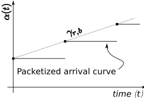
A straightforward option in bounding the sensing input at a given sensor node is based on its maximum sensing rate which is either due to the way the sensing unit is designed or limited to a certain value by the sensor network application’s task in observing a certain phenomenon. For example, it might be known that in a temperature surveillance sensor system, the temperature does not have to be reported more than once per second at most. To model such data arrivals in the SNC model, we now provide two options: a fluid and a discrete version. Thefluid modelfor each source nodeiis given by the frequently used token-bucket arrival curveαi(t) =γri,si(t) =
rit+si t >0
0 otherwise
with si as the size of a single data packet and ri as the maximum sensing rate of sensori. The more accurate dis-crete modelof it is given by a staircase function representing the discrete nature of the input in both packet size and sam-pling period. Mathematically, that curve is specified for each sensor nodeias:
αi(t) =si· „—
rit si
+ 1
«
[image:3.612.363.506.137.235.2]The more knowledge on the sensing operation and its char-acteristics is incorporated into the arrival curve for the sens-ing input the better the worst-case bounds become.
Figure 1: Maximum sensing rate arrival curve.
3.4
Minimum and Maximum Service Curve
The service curve depends on the way packets are sched-uled in a sensor node which mainly depends on link layer characteristics. More specific, the service curve depends on how the duty cycle and therefore the energy-efficiency goals are set.A typical and well-known example of a service curve from traditional traffic control in a packet-switched network is a rate-latency service curve [2]. The latency term nicely captures the characteristics induced by the application of a duty cycle concept. Whenever the duty cycle approach is applied there is the chance that sensed data or data to be forwarded just arrives after the last duty cycle is just over and thus a fixed latency occurs until the forwarding capacity is available again (for example, data is available after the TDMA slot just passed). In a simple duty cycle scheme this latency would need to be accounted for for all data transfers. For the forwarding capacity it is assumed that it can be lower bounded by a fixed rate which depends on transceiver speed, the chosen link layer protocol and the duty cycle. Ignoring the discrete nature due to packetization effects, we obtain the following fluid version of a minimum service curve at sensor nodei:
βi(t) =βfi,li(t) =fi[t−li]
+
(5)
where the notation [x]+equalsxifx≥0 and 0 otherwise. Here fi and li denote the forwarding rate and forwarding latency for sensor nodei.
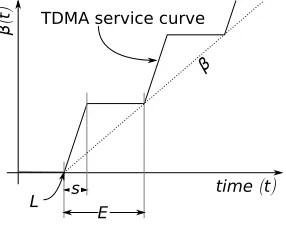
For the fluid version of the maximum service curve, we also assume a rate-latency curve, yet the latency must be less or equal and the forwarding rate greater or equal than the minimum service curve. In particular, for the remainder of the paper we assume the forwarding rate to be the same as for the minimum service curve and the latency to be 0, a frequent case, for example when using TDMA.
to be modelled by a period where no service is accumulated, whereas during the assigned slots, the full medium rate can be used . L denotes the initial delay,s is the TDMA slot length, andEis the duration of a TDMA cycle, also called theepoch. For comparison, a rate-latency approximation is shown as curveβ.
Figure 2: TDMA service curve
For the discrete version of the minimum service curve we thus assume exactly a curve as in Figure 2, whereas for the discrete version of the maximum service curve the initial delay is not incurred, so the curve is effectively shifted byL
to the left.
3.5
DISCO Network Calculator
A tool called The DISCO Network Calculator for au-tomatically performing the described SNC calculations is available [10]. The tool is especially useful if complex service and arrival curves have to be modeled. We used this tool to calculate the delay bounds in the evaluation section of the paper.
4.
SNC NETWORK DIMENSIONING
The SNC introduced in the previous section can only be used to describe a real deployment if specific properties are fulfilled by the sensor network. In this section these proper-ties are discussed in more detail and it is investigated how realistic sensor networks can fulfill these assumptions.
4.1
Network Structure
The SNC requires a network that forms a directed acyclic graph. This is the case in most sensor network deployments where data is collected at a central sink node. The resulting network topology in theses cases is a tree structure. It has to be noted that the SNC can also deal with cases where several sink nodes are used in the network (see [13]). In these cases the network is formed by combining several tree structures. The SNC cannot easily be applied in cases where all sensors communicate with each other and no clear direction of data flow is visible. For example, a scenario in which sensors in a field collaborate to track a vehicle would be a non-suitable scenario for the SNC.
Besides the need of having an acyclic graph structure, it is also required to know the shape of the network before the SNC can be applied. Ideally, the exact structure of the rout-ing tree is known at the point the SNC is applied. The SNC can deal as well with a topology that is only known approx-imately (for example, only the maximum hop distance and maximum number of child nodes for each node are known, see [9] for details). However, in this case the SNC calcu-lated worst-case bounds are further away from real-world
experienced bounds. The SNC could therefore be applied in scenarios where the network structure can be planned care-fully in advance.
A deployment fitting the aforementioned description could be, for example, a sensor network for process automation in a production plant. It is assumed that such scenarios consist of a relatively small number of nodes (a few dozen) which can be placed carefully. A non-fitting setting in contrast would be, for example, a scenario where thousands of nodes are dropped from a plane which need to organize autonomously.
4.2
Network Traffic
The first traffic requirement is given directly by the pre-viously described topology requirements. Traffic is assumed to flow from the sensors towards the sink(s). For many sen-sor network applications such a traffic characteristic is the normal mode of operation. The SNC presented in Section 3 does not model traffic flowing from the sink towards the sen-sors. However, if the network uses a static mode of operation this limitation is not an issue. For example, all nodes might be set up statically to report their findings to the sink. If communication from the sink to the nodes is required (for example, for configuration tasks) it can be argued that such traffic is magnitudes smaller and less frequent than the traf-fic created by the sensor nodes. Thus, the SNC calculation would still be valid. Another option to deal with sink-node traffic is to ensure that this traffic has no impact on the sensor-sink traffic which can be achieved by using TDMA-based MAC schemes (see section 4.3).
Besides knowledge on the general direction of the traffic, the SNC requires knowledge about the traffic generated by each node. To apply the SNC, an arrival curve which denotes the worst-case characteristics of the traffic emitted by the node has to be given. The better the worst-case bound of the traffic can be described, the better the SNC calculated bounds on the message transfer delay are. In many sensor network deployments, the traffic emitted by the nodes can be described fairly accurately. It might be known that sensors report at fixed periods and thus worst-case traffic bounds and actual traffic are identical (the arrival curve describes not the worst-case, it describes the actual case).
Thus, the SNC is useful in scenarios where traffic patterns are reasonably known and bounds on the traffic can be given. The SNC is not very useful in scenarios with random and fully unpredictable traffic patterns.
4.3
Message Forwarding
Operating System.
To achieve deterministic message pro-cessing, the operating system must be able to handle for-warding tasks in a deterministic way. Currently, event-driven operating systems such as TinyOS [15] are the pre-ferred choice for wireless sensor networks as they are very power-efficient. Unfortunately, these systems are in their standard configuration not able to provide the necessary de-terministic processing bounds. A TinyOS modification as described in [5] can be used to overcome this specific prob-lem. If such a modified operating system is used within the sensor network, the required deterministic message process-ing can be implemented.Medium Access Control.
An upper bound for the for-warding delay can only be given if the MAC protocol has a deterministic behavior. This can be achieved by using a TDMA-based MAC protocol in the sensor network. The SNC cannot be used in a sensor network that implements a contention-based MAC protocol as no upper bound for the message transfer delay can be given. TDMA-based protocols are available for wireless sensor networks and can be used in practical deployments (for example [6]). The MAC protocol defines as well the duty cycle which defines the communica-tion related power-efficiency of the sensor network.5.
SNC EVALUATION SETUP
The overall goal of the experimental evaluation is to com-pare SNC calculated message transfer delays and measured transfer delays in realistic deployments. This comparison is done in order to judge how useful the SNC is for dimension-ing a real world network.
To obtain useful results it is necessary to carry out the experimental measurements in a controlled setting. It is required to know exactly how experimental parameters in-fluence the measurements. In order to achieve this goal it was decided to carry out initial experiments in a simulation environment and not directly in a field trial. A simulation environment allows us to create a very realistic WSN behav-ior which is still fully controllable.
5.1
Setup
The network topology, traffic patterns and nodes’ message forwarding capabilities are chosen such that they fit the SNC requirements given in Section 4. Thus it is ensured that the simulated sensor network can actually be implemented in practice.
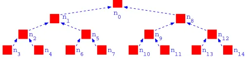
Network Topology.
The network structure used in the ex-perimental evaluation has a tree structure as shown in Fig. 3. The evaluated network consists of n = 15 sensor nodes. Static routing is used; child nodes route a message to their parent in the tree.n
0
n
1
n
2
n
3 n4
n
5
n
6 n7
n
8
n
9
n
10 n11
n
12
n
[image:5.612.53.307.622.683.2]13 n14
Figure 3: Network Structure
Message Forwarding.
It is assumed that the operating system can prioritize message processing. Sensing tasks are executed when no packet processing is required. Packets are queued behind all other packets currently awaiting ser-vice (FIFO). An operating system behavior equivalent to the TinyOS kernel modification described in [5] is modeled to achieve deterministic behavior.A simple TDMA based medium access control protocol is used in the network. The described protocol is based on ideas documented in [6] and can be used in a simple and well-controlled topology setting.
The base unit of the MAC protocol is the time unitepoch
E. The epoch is divided into mtime slots sm. A number of m≥n+ 1 time slots is required. Each of thensensors is assigned one time slot; the remaining time slot is used for contention-based access (for example broadcasts). A time slot is dedicated to exactly one node, thus, messages can be transmitted without collisions. Nodes must be awake for incoming messages during time slots allocated to their child nodes, their own time slot and for the contention based time slot. Thus, a node using this MAC protocol will have a duty cycle ofd= 4/min a binary tree topology.
At startup of the network, time synchronization among nodes is necessary and all nodes are in listening mode. The sink noden0announces the start of the epochEby sending
an epoch message in time slots0. The child nodes receive
the epoch message and thus are now synchronized with the epoch. Now the child nodes re-send the epoch message in their time slot. This process is repeated until every node received the epoch message. Thereafter, the TDMA scheme is set up and nodes can start forwarding messages to the sink without collisions. Periodically, the sink might refresh time synchronization by re-sending an epoch message.
For the experimental evaluation an epoch ofE= 100ms
andm= 20 is used. Thus, each time slotsmhas a duration of 5ms. We model a Chipcon CC2420 Zigbee transceiver with a transmission speed of 250kbps and a message size of 50byte. Thus, a message transmission has a duration of 1.6mswhich fits well in the selected slot size of 5ms.
It has to be noted that the protocol can be used in realistic deployments as large fields are not assumed. Furthermore, time slots are larger than the actual message transmission time. Therefore, time for packet processing is available and it is possible to cater for jitter in time synchronization. The described MAC protocol does not scale to large deployments. However, it is simple and efficient in small scenarios and can be implemented in a practical deployment.
The message forwarding used in the experimental setup can be bounded in the SNC by a rate-latency service curve as described by Equation (5). The forwarding rate is fi = 4kbit/s and the forwarding latency for nodeiisLi=E−
si= 95ms.
Network Traffic.
The traffic flows from the sensor nodes towards the sink. It is assumed that every node within the network creates periodic sensor reports with a frequency ofFor smallδ, all nodes in the field report their measurement at roughly the same time towards the sink. This could be the case if for example all sensors are triggered by the same observed phenomenon or because they are set-up to report findings periodically.
The network traffic used in the experimental setup can be bounded in the SNC by a maximum sensing rate arrival curve as described in section 3.3. For small δ all nodes in the field are closely synchronized and worst-case situations described by the SNC may be expected to be observed.
6.
SNC EXPERIMENTAL EVALUATION
The evaluation setup described in the previous section is used to evaluate the usefulness of the SNC calculations.
The jitter parameter δ in the traffic description is used as variable parameter in the experiments. The SNC can be used to calculate the worst-case bounds for the message transfer delay. By usingδ it is possible to “tune” the ex-perimental setup towards a worst-case behavior. It seems reasonable to assume that more packets close to the SNC calculated worst-case delay will be observed for small δ as all nodes become active at roughly same time. Ifδis large, few packets will experience the worst-case delay as network activity is spread over time.
6.1
SNC Calculated Message Transfer Delay
The worst-case message transfer delay is experienced in the experimental setup by messages transmitted from leaf nodes in the topology (see Fig. 3). The problem was set up using maximum sensing rate arrivals of one 50B packet every second with a 50B burst and service with a 95mslatency, 5msslot duration and a medium rate2 of 10kB/s.
TheDISCO Network Calculator was used to automatically perform the necessary SNC calculations.
The first calculations were done using fluid versions of arrival- and service curves, with the service curve model-ing a sustained rate of 100kB/s, 10kB per 100ms. A total flow analysis (TFA) summing up the per-hop delays yielded a delay bound of 5190ms. Next, the PMOO analysis was used, again with fluid models of arrival and service curves. The PMOOA resulted in a delay bound of 2367.5ms, obvi-ously a considerable improvement. To model the data flows more accurately, the curves were changed to their discrete versions as discussed in sections 3.3 and 3.4. A PMOO anal-ysis using these discrete versions of the curves resulted in a delay bound of 1490ms, while the TFA result decreased to 4100ms. Finally, by incorporating the maximum service curve concept, i.e. by modeling an upper bound on the ser-vice provided by the servers, the PMOO bound was further reduced to 890ms.3 Hence, we can observe a very signifi-cant improvement of the delay bound for this scenario using the advanced SNC concepts of PMOOA and the maximum service curve as well as the discrete versions of arrival- and service curves.
In other words, if the network is dimensioned according to the setup described in the previous section, all messages can be delivered in less than 890ms. If our application can deal with such a maximum delay our sensor network is
di-2The medium rate is chosen to reflect the transmission of at
most one 50B-packet per slot.
3The TFA did not improve when the maximum service curve
was used in the TDMA model.
mensioned correctly. If the delay is too high, we might want to increase the forwarding rate (e.g. by reducing the epoch
E of the MAC layer). If the delay is lower than required we might want to decrease the forwarding capabilities of the nodes which would result in better energy savings (the duty cycle will improve).
The open question is now how close really observed de-lays are to the calculated bound of 890ms. In addition, it is important to find out how many packets will actually expe-rience this worst-case delay. These remaining questions will be addressed by the measurements described in the next subsection.
6.2
Measured Message Transfer Delays
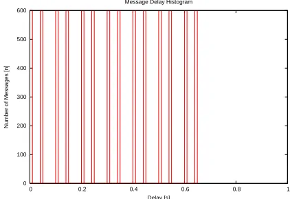
The parameterδ is used as variable parameter in the ex-periments. The message transfer delay di of all packets is recorded during the experiments. The delay is measured from the time the message is generated until it reaches the sink noden0. An experiment duration is 600 seconds. Thus,with all 14 nodes reporting once a second, 8400 messages are generated during one experiment4. Values betweenδ= 0ms
andδ= 500msare used as jitter within the experiments. Fig. 4 shows the delay histogram forδ= 0ms. In this case, all nodes in the field report at exactly the same time, at the beginning of an epochE. As a result, the delay distribution is very homogeneous as forwarding queues in the network are always filled in the same way. Basically, the network is free of any random event.
The measured worst-case delay isdmax = 640ms. This worst-case delay is experienced by 600 messages during the experiment. These messages are generated by node n14. A
message generated byn14takes 6 epochsEto travel to node n8 and being scheduled for transmission as messages from n14queue behind all other messages generated in the branch.
Finally from noden8 ton040msare added as noden8uses
time slot number 8 (slot size 5ms).
0 100 200 300 400 500 600
0 0.2 0.4 0.6 0.8 1
Number of Messages [n]
[image:6.612.328.539.451.596.2]Delay [s] Message Delay Histogram
Figure 4: Delay histogram; fully synchronized net-work (δ= 0ms).
As expected, all measured delays are below the SNC calcu-lated worst-case bound of 890ms. The calculated worst-case bound of 890msis 39% above the measured worst-case de-lay of 640ms. The measured worst-case delay is experienced by 7.1% of all messages. In addition, 28.6% of the messages
4Not all 8400 messages might reach the sink as some
experience a delay between 445ms and 890ms (a window describing messages which experience more than half of the SNC calculated worst-case bound).
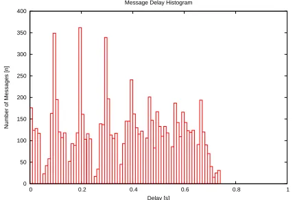
Fig. 5 shows the delay histogram forδ = 50ms. In this case, all nodes have a slight offset when generating mes-sages. Again, all measured delays are below the SNC cal-culated worst-case bound of 890ms. The calculated worst-case bound of 890msis 20.4% above the measured delay of 739ms(This message was generated by noden11). It has to
be noted that the measured worst-case delay is significantly higher than forδ= 0. Thus, the fully synchronized network with δ = 0 does not represent - as one might think - the worst possible scenario. A slight jitter in message genera-tion patterns enables unfavorable scheduling situagenera-tions. In this experimental run, 36.6% of the messages experience a delay between 445msand 890ms.
0 50 100 150 200 250 300 350 400
0 0.2 0.4 0.6 0.8 1
Number of Messages [n]
Delay [s] Message Delay Histogram
[image:7.612.327.542.280.427.2]Figure 5: Delay histogram; synchronized network (δ= 50ms).
Fig. 6 shows the delay histogram forδ= 250ms. In this case, nodes are not closely synchronized regarding message generation. All measured delays are below the SNC calcu-lated worst-case bound of 890ms. The calculated worst-case bound of 890msis 6.6% above the measured worst-case de-lay of 835ms(This message was generated by noden11). In
this experimental run, 30.7% of the messages experience a delay between 445msand 890ms.
0 50 100 150 200 250 300
0 0.2 0.4 0.6 0.8 1
Number of Messages [n]
Delay [s] Message Delay Histogram
Figure 6: Delay histogram; un-synchronized net-work (δ= 250ms).
Fig. 7 shows a summary of all experimental runs with
differentδ. The abscissa shows the simulation runs for dif-ferentδ(0ms < δ <500ms); the ordinate depicts the delay. The figure shows the calculated worst-case delay of 890ms, the worst-case delay observed during measurements and the 90%-quantile of measured delays. 10% of the delay measure-ments in the experiment run are above and 90% are below the 90%-quantile value. Thus, the 90%-quantile graph gives a quantitative indication of how close the measured delays are to the SNC calculated worst-case bound.
All measured delays are below the SNC calculated worst-case bound of 890ms. Measured worst-case delay and calcu-lated worst-case delay are closest forδ= 475ms. Here, the calculated worst-case bound of 890ms is only 2.7% above the measured worst-case delay of 867ms.
The graphs show that the worst-case is relatively indepen-dent of the jitterδ. Even for a high jitter a high worst-case delay can still occur. However, the 90%-quantile is dropping slightly with the amount of jitter introduced. This indicates that message transfer delays close to the calculated worst-case bounds are less likely to occur.
0 0.2 0.4 0.6 0.8 1
0 100 200 300 400 500
Delay [s]
Jitter Delta [ms] Message Transfer Delays
Measured Worst Case 90-Quantile of Measured Delays SNC Calculated Worst Case
Figure 7: Measured worst-case delays in dependence ofδ (0ms < δ <500ms).
Fig. 8 shows the percentage of messages that experience a delay between 445msand 890msin dependence of the jitter
δ. These messages experience more than half of the SNC calculated worst-case bound. The graph shows that lower data transport delays are measured with increasing jitter.
0 20 40 60 80 100
0 100 200 300 400 500
Percent [%]
Jitter Delta [ms]
Percent of Packets within 50% of SNC Worst Case Delay
Packets within 50% of SNC Delay
Figure 8: Percentage of messages with455ms < di<
[image:7.612.65.282.523.668.2] [image:7.612.327.542.533.680.2]6.3
Findings
Our experiments show that the SNC calculated worst-case delay is close to the experienced delays in a realistic applica-tion setting. Actual measured delays in the experiment can be predicted by the SNC as close as 2.7% (forδ= 475ms).
More than 30% (for 10ms < δ <250ms) of messages ex-perience a delay between 445msand 890ms. This delay win-dow describes messages which experience more than half of the SNC calculated worst-case bound. If the sensor network would be dimensioned without using a dimensioning tool such as the SNC and a provisioning error of 50% is made, about 30% of the messages will not be delivered in time and might have to be counted as loss. Losses of this magnitude, in addition to packet losses due to noisy channels, are too high for many sensor network applications that require per-formance guarantees. Dimensioning errors of 50% are easily possible if no useful dimensioning tool is available. Over-provisioning by several orders would reduce the risk of error but is not a viable option in resource constrained wireless sensor networks. Usually, over-provisioning would translate to higher energy consumption and, thus, shorter network lifetime.
7.
CONCLUSION
The goal of this paper was to shed light on the question of whether the SNC can be a valuable tool for the dimensioning of WSNs. The presented results show that SNC predicted worst-case message transfer delay bounds are very close to measured delays in simulations of restricted, yet realistic WSNs deployment scenarios. For example, a difference of only 2.7% between calculated and measured worst-case de-lay was observed for one specific experiment and in all ex-periments it was never off by large. Thus, we validated that the SNC can be used as a reasonably accurate dimension-ing tool for the class of wireless sensor network applications investigated in this paper. It should be noted that this pos-itive answer to our basic question on the suitability of the SNC as a WSN dimensioning tool is also a result of the improvements for the basic SNC (PMOO analysis method, maximum service curve, discrete modeling) that we intro-duced in this paper.
We believe that the SNC can be used to derive practical design guidelines for a wireless sensor network that requires strict message transfer delay guarantees. The SNC can be used as dimensioning tool to avoid a) over-provisioned sensor networks b) undesired message transfer delays.
We plan to repeat the presented measurements using a practical deployment instead of a simulated sensor network environment. We expect that these real-world measure-ments will confirm the presented simulation results.
8.
REFERENCES
[1] T.R. Abdelzaher, S. Prabh, and R. Kiran. On real-time capacity limits of multihop wireless sensor networks. InRTSS ’04: Proceedings of the 25th IEEE International Real-Time Systems Symposium. IEEE, December 2004.
[2] Jean-Yves Le Boudec and Patrick Thiran.Network calculus: a theory of deterministic queuing systems for the internet. Springer-Verlag New York, Inc., New York, NY, USA, 2001.
[3] C.-F. Chiasserini and M. Garetto. Modeling the performance of wireless sensor networks. InProc. IEEE INFOCOM, March 2004.
[4] R. L. Cruz. SCED+: Efficient management of quality of service guarantees. InProc. IEEE INFOCOM, volume 2, pages 625–634, March 1998.
[5] Cormac Duffy, Utz Roedig, John Herbert, and Cormac J. Sreenan. Adding Preemption to TinyOS. In Proceedings of the The Fourth Workshop on Embedded Networked Sensors (EmNets2007), Cork, Ireland. ACM Press, June 2007.
[6] L. van Hoesel and P. Havinga. A lightweight medium access protocol (LMAC) for wireless sensor networks. InINSS04, Tokyo, Japan, June 2004.
[7] Anis Koubaa, Mario Alves, and Eduardo Tovar. Modeling and worst-case dimensioning of cluster-tree wireless sensor networks. InRTSS ’06: Proceedings of the 27th IEEE International Real-Time Systems Symposium, pages 412–421, Washington, DC, USA, 2006. IEEE Computer Society.
[8] Jens Schmitt and Utz Roedig. Sensor Network Calculus - A Framework for Worst Case Analysis. In Proceedings of IEEE/ACM International Conference on Distributed Computing in Sensor Systems (DCOSS’05), Marina del Rey, USA, pages 141–154. Springer, LNCS 3560, June 2005. ISBN 3-540-26422-1. [9] Jens Schmitt and Utz Roedig. Worst Case
Dimensioning of Wireless Sensor Networks under Uncertain Topologies. InProceedings of 3rd International Symposium on Modeling and Optimization in Mobile, Ad Hoc, and Wireless Networks (WiOpt’05), Workshop on Resource Allocation in Wireless Networks, Riva del Garda, Italy. IEEE, April 2005. ISBN 0-9767294-0-7. [10] Jens B. Schmitt and Frank A. Zdarsky. The DISCO
Network Calculator - A Toolbox for Worst Case Analysis. InProceedings of the First International Conference on Performance Evaluation Methodologies and Tools (VALUETOOLS’06), Pisa, Italy. ACM, November 2006.
[11] Jens B. Schmitt, Frank A. Zdarsky, and Markus Fidler. Delay Bounds under Arbitrary Multiplexing. Technical Report 360/07, University of Kaiserslautern, Germany, July 2007.
[12] Jens B. Schmitt, Frank A. Zdarsky, and Ivan Martinovic. Performance Bounds in Feed-Forward Networks under Blind Multiplexing. Technical Report 349/06, University of Kaiserslautern, Germany, April 2006.
[13] Jens B. Schmitt, Frank A. Zdarsky, and Utz Roedig. Sensor Network Calculus with Multiple Sinks. In Proceedings of IFIP NETWORKING 2006, Workshop on Performance Control in Wireless Sensor Networks, Coimbra, Portugal, pages 6–13. Springer LNCS, May 2006. ISBN 972-95988-5-1.
[14] J.A. Stankovic, T. Abdelzaher, C. Lu, L. Sha, and J.Hou. Real-time communication and coordination in embedded sensor networks.Proceedings of the IEEE, 91:1002–1022, 2003.