An Algorithm to Construct Decision Tree for Machine Learning based on Similarity Factor

An Algorithm to Construct Decision Tree for Machine

Learning based on Similarity Factor

Neha Patel

CSE Department BUIT, BU Bhopal

Divakar Singh

Head of CSE Department BUIT, BU Bhopal

ABSTRACT

Data mining is one of the most important steps of the knowledge discovery in databases process and is considered as significant subfield in knowledge management. A classification of the data mining methods would greatly simplify the understanding of the whole space of available methods. Decision tree learning algorithm has been successfully used in expert systems in capturing knowledge. Most decision tree classifiers are designed to classify the data with categorical or Boolean class labels. To the best of our knowledge, no previous research has considered the induction of decision trees from data with data dissimilarities. This work proposes a novel classification algorithm for learning decision tree classifiers from data using dissimilarities with less complexity and less time to construct decision tree.

KEYWORDS: Data Mining, Classification, Decision Tree, ID3 Algorithm.

1.

INTRODUCTION

Data mining is a collection of techniques for efficient automated discovery of in the past unknown, valid, novel, useful and understandable patterns in big databases. The patterns must be actionable so that they may be used in an enterprise‟s decision making process. In recent years, there has been increasing interest in the use of data mining to investigate scientific questions within learning research, an area of inquiry termed educational data mining [1].

Knowledge discovery in databases (KDD) [2], often called data mining, extracting information and patterns from data in big data base. The core functionalities of data mining are applying various techniques to identify nuggets of information of decision making knowledge in bodies of data [2]. From the last decades, data mining and knowledge discovery applications have important significance in decision making and it has become an essential component in various organizations and fields. The field of data mining has been greater than before day by day in the areas of human life with various integrations and advancements in the fields of Statistics, Databases, Machine Learning [3], Pattern Reorganization, Artificial Intelligence and Computation capabilities etc.

There are several algorithms which are also using genetic and fuzzy set are also applied in these areas [15]. Combine the fuzzy and search capabilities of Genetic Algorithms (GAs) may improve the optimal fuzzy rule and improve the rule generation also [15].

The improved ID3 based on weighted modified information gain called ωID3 [16] judges whether one condition attribute need to modify by computing objectively. Choosing splitting attributes blindly in reference has been improved and subjective evaluating using users' interestingness in reference is also overcome. Because ωID3 takes the relevance among attributes into account, the classification precision is enhanced. The experiment shows that ωID3 classification precision is superior to ID3 obviously.

2.

LITERATURE SURVEY

Researchers have developed various classification techniques over a period of time with enhancement in performance and ability to handle various type of data. A number of important algorithms are discussed below.

2.1 Oblique Decision Tree

Tree induction algorithms like Id3 and C4.5 create decision trees that take into account only a single attribute at once. For each node of the decision tree an attribute is selected from the feature space of the dataset which brings maximum information gain by splitting the data on its distinct values. The information gain is calculated as the difference between the entropy of the initial dataset and the sum of the entropies of each of the subsets after the split.

2.2 CART

Classification and regression tree (CART) proposed by Breiman et al. [7] constructs binary trees which is also refer as Hierarchical Optimal Discriminate Analysis (HODA). CART is a non-parametric decision tree learning technique that produces either classification or regression trees, depending on whether the reliant variable is categorical or numeric, in that order. The word binary implies that a node in a decision tree can only be split into two groups. CART uses gini index as adulteration measure for selecting attribute. The attribute with the major reduction in impurity is used for splitting the node's proceedings. CART accepts data with numerical or categorical values and also handles missing attribute values. It helpful to uses cost-complexity pruning and generate regression trees.

2.3 CART-LC

The first oblique decision tree algorithm to be proposed was CART with linear combinations .Breiman, Friedman, Olshen, and Stone (1984) introduced CART with linear combinations (CART-LC) as an option in their popular decision tree algorithm CART. At each node of the tree, CART-LC iteratively finds locally optimal values for each of the coefficients. Hyperplanes are generate and test until the marginal benefits become smaller than a constant [5].

2.4 C4.5

C4.5 is an algorithm used to generate a decision tree developed by Ross Quinlan. C4.5 is an expansion of Quinlan‟s earlier ID3 algorithm. The decision trees generate by C4.5 can be used for classification, and for this cause C4.5 is often referred to as a statistical classifier [7]. C4.5 algorithm uses information gain as splitting criteria. It can allow data with categorical or numerical values. To knob continuous values it generates threshold and then divides attributes with values above the threshold and values equal to or below the threshold. C4.5algorithm can simply handle missing value. As missing attribute values are not utilize in gain calculations by C4.5.

23 C5.0 algorithm is an addition of C4.5 algorithm which is also

extension form of ID3. It is the classification algorithm which applies in large data set. It is better than C4.5 on the speed, memory and the efficiency. C5.0 model moving by splitting the sample based on the field that provides the maximum information gain. The C5.0 model can split samples on root of the biggest information gain field. The model subset that is get from the former split will be split afterward. The procedure will continue until the sample subset cannot be split and is usually according to one more field. Finally, examine the lowest level split, sample subsets that don‟t have notable contribution to the model will be discarded. C5.0 is without difficulty handled the multi value attribute and missing attribute from data set [8].

2.6 Hunt’s Algorithm

Hunt‟s algorithm generates a Decision tree by top-down or divides and conquers move toward. The sample/row data contains supplementary class, use an attribute test to split the data into slighter subsets. Hunt‟s algorithm maintains optimal split for every stage according to some threshold value as greedy fashion [9].

3.

PROPOSED METHOD

In this proposed method we are using modified ID3 algorithm for decision tree. Attribute selection plays important role in efficient decision tree construction for root to bottom node.

Decision trees can handle high dimensional data. Their illustration of acquired knowledge in tree form is intuitive and generally easy to take in by humans. The learning and classification steps of decision tree induction are simple and fast.

The algorithm through introducing attribute-importance emphasizes the attributes with less values and higher import, adulterate the attributes with more values and lower importance, and solve the classification defect of inclining to choose attributions with more values. The analysis of the experimental data show that the improved ID3 algorithm gets more reasonable and more effective classification rulesˊ In order to increase the attributes which have fewer values and high importance, and reduce the attributes which have more values and have low import, improved ID3 algorithm based on attribute importance is proposed in this paper.

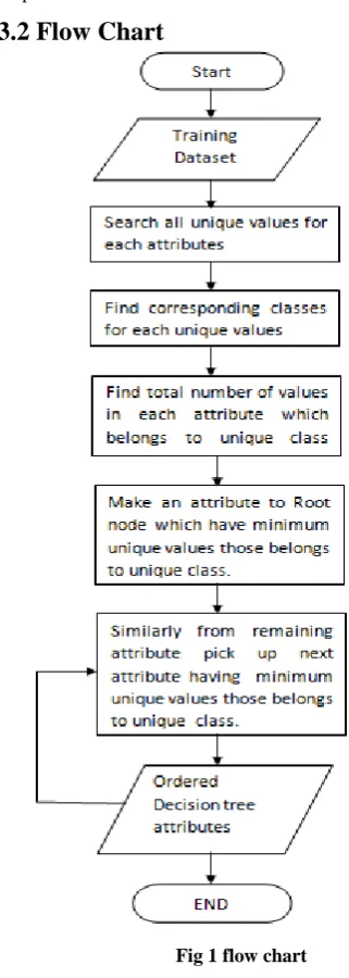
In this proposed method first of all we analyze hole training data and find the attribute for root node on the basis of less dissimilarity with respect to class. Similarly find next node for 2nd level from remaining attributes, and so on. Fig 1 shows flow chart of this work Macintosh, use the font named Times. Right margins should be justified, not raggedy.

3.1 Algorithm

Step 1: select training dataset for learning.

Step 2: find mapping between every individual attribute to classes.

Step 3: find all possible values for every attribute and that corresponding possible classes.

Step 4: then count values of each attributes which belongs to unique class.

Step 5: Make root node to that attribute which have minimum number of values having unique class.

Step 6: Similarly select other attribute for next level in decision tree from remaining attribute on the basis of minimum number of values having unique class.

Step 7: Exit

3.2 Flow Chart

Fig 1 flow chart

4.

RESULT AND ANALYSIS

4.1

ID3 Algorithm

ID3 algorithm is explained here using the classic „Play Tennis‟ example. Table 1 shows the training dataset. The attributes are Outlook, Temp, Humidity, Wind, and Play Tennis. The Play Tennis is the target attribute shown in figure 2.

Table 1. Training dataset

Outlook Temp Humidity Wind

Sunny Hot High Weak

Sunny Hot High Strong

Overcast Mild High Weak

Rain Mild High Weak

Rain Cool Normal Weak

Overcast Cool Normal Strong

Sunny Mild High Weak

Sunny Cool Normal Weak

Rain Mild Normal Weak

Sunny Mild Normal Strong

Overcast Mild High Strong

Overcast Hot Normal Weak

Rain Mild High Strong

Calculating entropy based on the above formulas gives: - Entropy ([9+,5-]) = − (9 /14)log (9 /14) (5/14)log (5/14) = 0.940

Gain(S,Humidity) =0.151

Gain(S,Temp)=0.029

Gain(S, Outlook) = 0.246

Based on the above calculations attribute outlook is selected and algorithm is repeated recursively. The decision tree for the algorithm is shown in Figure 2

STEP BY STEP CALCULATIONS: STEP 1:“example” set s

The set s of 14 examples with 9 yes and 5 no then

Entropy (S) = -(9/14) Log2 (9/14) – (5/14) Log2 (5/14) = 0.940

STEP 2: Attribute weather

Weather value can be sunny, cloudy, and rainy.

Weather =sunny is of occurrence 5

Weather = cloudy is of occurrences 4

Weather = rainy is of occurrences 5

Weather = sunny, 2 of the examples are “yes” and 3 are “no”

Weather = cloudy, 4 of the examples are “yes” and 0 are “no”

Weather = rainy, 3 of the examples are “yes” and 2 are “no”

Entropy (Ssunny) = -(2/5)xlog2(2/5) – (3/5)xlog2(3/5) = 0.970950

Entropy (Scloudy) = -(4/4)xlog2(4/4) – (0/4) xlog2 (0/4) = 0

Entropy (Ssunny) = -(3/5)xlog2(3/5) – (2/5) xlog2 (2/5) = 0.970950

Gain (S, weather) = Entropy (S) – (5/14) x Entropy (S sunny)

- (4/14) x Entropy (Scloudy)

- (5/14) x Entropy (Srainy)

= 0.940 – (5/14) x 0.97095059 – (4/14) x 0 – (5/14) x 0. 97095059

= 0.940 – 0.34676 – 0 – 0.34676 = 0.246

STEP 3: Attribute temperature

Temp value can be hot, medium or cold.

Temp = hot is of occurrences 4

Temp = medium is of occurrences 6

Temp = cold is of occurrences 4

Temp =hot, 2 of the examples are “yes” and 2 are “no”

Temp =medium, 4 of the examples are “yes” and 2 are “no”

Temp =cold, 3 of the examples are “yes” and 1 are “no”

Entropy (Shot) = - (2/4) x log2 (2/4) – (2/4) x log2 (2/4) = - 0.99999999

25

4.2 Solution by Proposed Method

First of all find unique values of all attribute and corresponding classes from where they belong.

Table 2

Outlook

Sunny No

Yes

Rain No

Yes

Overcast Yes

Table 3

Temp

Hot No

Yes

Mild No

Yes

Cool No

Yes

Table 4

Humidity

High No

Yes

Normal No

Table 5

Wind

Weak No

Yes

Strong No

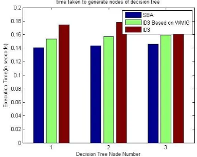
Here we have seen that outlook have 1 unique value which belongs to unique class. Similarly Temp, Humidity and Wind have 0 unique values which belong to unique class. So Outlook is a root node because it has maximum values. Fig 3 shows comparison of time taken to generate first 3 nodes in decision tree by proposed method.

Fig 3. Comparison graph for time taken to generate nodes of decision tree for dataset.

Fig 4 shows performance with respect to time among ID3, ID3 based on WMIG and SBA. And here we can clearly see that SBA is more efficient than ID3 and ID3 based on WMIG and it gives better result

Fig 4 comparison of performance of ID3, ID3 based on WMIG and MID3 algorithm

5.

CONCLUSION

The decision tree method is increasing in popularity for both classification and prediction. It can also be used for cluster analysis and time series in some situations. The main advantages of this method are its simplicity, non-parametric nature, robustness, and the ability to process both quantitative and qualitative variables. Decision trees can be easily converted to classification rules that can be expressed in common language.

An SBA algorithm is presented to overcome deficiency of general ID3 algorithm which tends to take attributes with many values. The presented algorithm makes the constructed decision tree more clear and understandable because it has less complexity.

6.

ACKNOWLEDGMENTS

I am thankful to Mr. Divakar Singh (HOD Deptt. Of CSE)BUIT, BU Bhopal for supporting this work.

7.

REFERENCES

[1] Gorunescu, F, Data Mining: Concepts, Models, and Techniques, Springer, 2011.

[2] Han, J., and Kamber, M. , Data mining: Concepts and techniques, Morgan-Kaufman Series of Data Management Systems San Diego:Academic Press, 2001.

[3] Neelamadhab Padhy, Dr. Pragnyaban Mishra and Rasmita Panigrahi, “The Survey of Data Mining Applications and Feature Scope, International Journal of Computer Science, Engineering and Information Technology (IJCSEIT)”, vol.2, no.3, June 2012.

[4] Shreerama Murthy,Simon Kasif,Stivon Salzberg,Richard Beigel,“Oc1:Randomized Induction Of Oblique Decision Tree”

[5] Leo Breiman, Jerome H. Friedman, Richard A. Olshen, and Charles J. Stone. Classification and Regression Trees. Wadsworth International Group, Belmont, California, 1984.

[6] Zhu Xiaoliang, Wang Jian YanHongcan and Wu Shangzhuo Research and application of the improved algorithm C4.5 on decision tree, 2009.

[7] Prof. Nilima Patil and Prof. Rekha Lathi, Comparison of C5.0 & CART Classification algorithms using pruning technique, 2012.

[8] Baik, S. Bala, J., A Decision Tree Algorithm For Distributed Data Mining, 2004.

[9] Girija, D.K.S.; Shashidhara, M.S., "Data mining techniques used for uterus fibroid diagnosis and

prognosis," Automation, Computing, Communication, Control and Compressed Sensing (iMac4s), International Multi-Conference on , vol., no., pp.372,376, 22-23, 2013.

[10]Al Jarullah, A.A., "Decision tree discovery for the diagnosis of type II diabetes," Innovations in Information Technology (IIT), 2011 International Conference on , vol., no., pp.303,307, 25-27 April 2011.

[11] Mai Shouman, Tim Turner, Rob Stocker, “using data mining techniques in heartdisease diagnosis and treatment”, Egypt Conference on Electronics, Communications and Computers, 2012.

[12] Parvathi I, Siddharth Rautaray, “Survey on Data Mining Techniques for the Diagnosis of Diseases in Medical Domain”, International Journal of Computer Science and Information Technologies, Vol. 5 (1) , 838-846, 2014.

[13]Varsha Mashoria , Dr. Anju Singh, “A Survey of Mining Association Rules Using Constraints”, International Journal Of Computers & Technology.

[14]Jyotsna Bansal, Divakar Singh, Anju Singh, “An Efficient Medical Data Classification based on Ant Colony Optimization”, International Journal of Computer Applications (0975 – 8887)Volume 87 – No.10, February 2014.

[15]O. Cordón, F. Gomide, F. Herrera, F. Hoffmann, and L. Magdalena, “Ten years of genetic fuzzy systems: current framework and new trends,” Fuzzy Sets Syst., vol. 141, pp. 5–31, 2004.