Gaussian Barebones Differential Evolution with
Random-type Gaussian Mutation Strategy
Hung-Ching Lu
1, Ming-Feng Yeh
2,*, Yu-Wei Lu
11Department of Electrical Engineering, Tatung University, Taiwan
2Department of Electrical Engineering, Lunghwa University of Science and Technology, Taiwan
Copyright©2016 by authors, all rights reserved. Authors agree that this article remains permanently open access under the terms of the Creative Commons Attribution License 4.0 International License
Abstract This study attempts to propose a random-type
Gaussian mutation strategy to improve the solution accuracy of Gaussian barebones differential evolution (GBDE). The proposed Gaussian mutation strategy is not only parameter free, but also employed to enhance the population diversity and global searching ability of the original mutation strategy. The search performance of GBDE with the proposed mutation strategy is compared with two standard DEs (DE/rand/1 and DE/best/1), the original GBDE and its modified version in terms of solution accuracy. Simulation results on two real-world optimal control problems given in IEEE - CEC 2011 evolutionary algorithm competition demonstrate the effectiveness of the proposed GBDE algorithm.Keywords Differential Evolution, Mutation Strategy,
Gaussian Sampling, Gaussian Barebones Differential Evolution1. Introduction
Differential evolution (DE) algorithm, proposed by Storn and Price in 1995, is a simple yet powerful evolutionary algorithm (EA) for global optimization problems in the continuous search domain [1]. The performance of DE algorithm is generally sensitive to the mutation strategy and the respective control parameters such as the scale factor F, the crossover rate Cr, and the population size Np [2]. In order to minimize the effects of control parameters, a number of adaptive DE variants have been proposed in the past several years [3]-[5]. In addition, rather than using complex adaptive or self-adaptive mechanisms, barebones DE (BBDE) [6] and Gaussian barebones DE (GBDE) [7] are two almost parameter free DE variants. Both of them could achieve a good balance between exploration and exploitation in the search process.
GBDE is based on the Gaussian sampling. As indicated in [7], the Gaussian sampling is a fine tuning procedure
which starts during explorations and is continued to exploitation. This can be beneficial for the search of many evolutionary optimization algorithms. The Gaussian mutation strategy is implemented by a Gaussian random function with mean 𝜇𝜇= (𝐱𝐱𝑏𝑏𝑏𝑏𝑏𝑏𝑏𝑏,𝐺𝐺+𝐱𝐱𝑖𝑖,𝐺𝐺)/2 and standard
deviation 𝜎𝜎=�𝐱𝐱𝑏𝑏𝑏𝑏𝑏𝑏𝑏𝑏,𝐺𝐺− 𝐱𝐱𝑖𝑖,𝐺𝐺�, where 𝐱𝐱𝑏𝑏𝑏𝑏𝑏𝑏𝑏𝑏,𝐺𝐺 and 𝐱𝐱𝑖𝑖,𝐺𝐺
represent the best vector and the i-th target vector at the G-th generation, respectively. GBDE also employs the crossover schemes used in the classical DEs. Without loss of generality, this study only considers the binomial crossover scheme. In [7], Wang et al also proposed the hybridization of Gaussian mutation and DE/best/1 to balance the global search ability and convergence rate. Such a GBDE variant is termed the modified GBDE (MGBDE). In MGBDE, each vector is randomly assigned a mutation strategy (either Gaussian mutation or DE/best/1) during the population initialization. The assigned mutation strategy for each vector does not change during the search process. About 50% of the vectors follow the behavior of DE/best/1, while the remaining 50% follow the GBDE.
Gaussian mutation strategy is a kind of the best-so-far solution-based strategies. That is, the best solution will guide the direction of evolutionary search, and then might lead to the problem of premature convergence caused by the reduced population diversity. Among the classic DE strategies, “DE/rand/1” strategy, which is usually less greedy, has slower convergence speed, and is more reliable than the strategies based on the best-so-far solution [1,5,8]. This gives rise to the motivation to apply “DE/rand/1” strategy to Gaussian mutation strategy to propose a newly mutation strategy termed the random-type Gaussian mutation strategy. The newly developed random-type Gaussian mutation strategy is attempted to preserve the diversity of the population and the problem of premature convergence can be alleviated.
favorably with the original GBDE and MGBDE as well as two classical DEs, “DE/rand/1” and “DE/best/1”.
The remainder of this paper is organized as follows. Section 2 briefly describes GBDE and its modified version MGBDE. The proposed random-type Gaussian mutation strategy is described in Section 3. Section 4 presents the search performance of the proposed approaches on two optimal control problems. Finally, Section 5 contains some conclusions of this study.
2. DE Algorithms, GBDE and MGBDE
2.1. DE Algorithms
Like other EAs, DE algorithm starts with a randomly generated initial population vector within the search space. After initialization, DE then enters a loop of evolutionary operations: mutation, crossover, and selection as follows [1,4]. Let xi,G = (x1i,G, x2i,G, ..., xDi,G) be a target (solution)
vector in generation G, where i = 1, 2, …, NP (Np =
population size).
Mutation: For each target vector xi,G, DE employs the
mutation operation to produce a mutant vector vi,G. The
following strategies are five most frequently used schemes: DE/rand/1:
𝐯𝐯𝑖𝑖,𝐺𝐺=𝐱𝐱𝑟𝑟1,𝐺𝐺+𝐹𝐹(𝐱𝐱𝑟𝑟2,𝐺𝐺− 𝐱𝐱𝑟𝑟3,𝐺𝐺) (1)
DE/best/1:
𝐯𝐯𝑖𝑖,𝐺𝐺 =𝐱𝐱𝑏𝑏𝑏𝑏𝑏𝑏𝑏𝑏,𝐺𝐺+𝐹𝐹(𝐱𝐱𝑟𝑟1,𝐺𝐺− 𝐱𝐱𝑟𝑟2,𝐺𝐺 (2)
DE/current-to-best/1:
𝐯𝐯𝑖𝑖,𝐺𝐺=𝐱𝐱𝑖𝑖,𝐺𝐺+𝐹𝐹(𝐱𝐱𝑏𝑏𝑏𝑏𝑏𝑏𝑏𝑏,𝐺𝐺− 𝐱𝐱𝑖𝑖,𝐺𝐺) +𝐹𝐹(𝐱𝐱𝑟𝑟1,𝐺𝐺− 𝐱𝐱𝑟𝑟2,𝐺𝐺) (3)
DE/rand/2:
𝐯𝐯𝑖𝑖,𝐺𝐺=𝐱𝐱𝑟𝑟1,𝐺𝐺+𝐹𝐹�𝐱𝐱𝑟𝑟2,𝐺𝐺− 𝐱𝐱𝑟𝑟3,𝐺𝐺�+𝐹𝐹�𝐱𝐱𝑟𝑟4,𝐺𝐺− 𝐱𝐱𝑟𝑟5,𝐺𝐺� (4)
DE/best/2:
𝐯𝐯𝑖𝑖,𝐺𝐺 =𝐱𝐱𝑏𝑏𝑏𝑏𝑏𝑏𝑏𝑏,𝐺𝐺+𝐹𝐹�𝐱𝐱𝑟𝑟1,𝐺𝐺− 𝐱𝐱𝑟𝑟2,𝐺𝐺�+𝐹𝐹�𝐱𝐱𝑟𝑟4,𝐺𝐺− 𝐱𝐱𝑟𝑟5,𝐺𝐺� (5)
where the indices r1, r2, r3, r4, and r5 are distinct integers randomly generated from the set {1, 2, …, 𝑁𝑁𝑝𝑝}\{i}, (𝐱𝐱𝑟𝑟1,𝐺𝐺− 𝐱𝐱𝑟𝑟2,𝐺𝐺) or �𝐱𝐱𝑟𝑟2,𝐺𝐺− 𝐱𝐱𝑟𝑟3,𝐺𝐺� is a difference vector to
mutate the base vector, 𝐱𝐱𝑏𝑏𝑏𝑏𝑏𝑏𝑏𝑏,𝐺𝐺 represents the best vector at
the 𝐺𝐺-th generation, and the parameter F is called the scaling factor.
Crossover: Crossover operation is applied to combine the target vector xi,G and its corresponding mutant vector vi,G to
generate a trial vector ui,G = (u1i,G, u2i,G, ..., uDi,G). The
widely-used binomial crossover scheme is defined as follows.
𝑢𝑢𝑗𝑗𝑖𝑖,𝐺𝐺=�𝑥𝑥𝑣𝑣𝑗𝑗𝑖𝑖,𝐺𝐺, if �𝑟𝑟𝑟𝑟𝑟𝑟𝑟𝑟𝑗𝑗≤ 𝐶𝐶𝑟𝑟� or (𝑗𝑗=𝑗𝑗𝑟𝑟𝑟𝑟𝑟𝑟𝑟𝑟)
𝑗𝑗𝑖𝑖,𝐺𝐺, otherwise (6)
for j = 1, 2, …, D, where randj is a randomly chosen real
number within the range of (0, 1), Cr is the crossover rate and jrand∈ {1,2, …, D} is a randomly chosen index which
ensures that the trial vector ui,G gets at least one element
from vi,G.
Selection: The selection operation selects the better one from the target vector xi,G and the trial vector ui,G according
to their fitness values. That is
𝐱𝐱𝑖𝑖,𝐺𝐺+1=�𝐱𝐱𝐮𝐮𝑖𝑖,𝐺𝐺, if 𝑓𝑓(𝐮𝐮𝑖𝑖,𝐺𝐺)≤ 𝑓𝑓(𝐱𝐱𝑖𝑖,𝐺𝐺)
𝑖𝑖,𝐺𝐺, otherwise (7)
Using this greedy selection scheme, all individuals of the next generation are better than the individuals of the current population.
2.2. GBDE and MGBDE
In the GBDE, the Gaussian mutation strategy is defined as follows.
𝐯𝐯𝑖𝑖,𝐺𝐺 =𝑁𝑁(𝜇𝜇,𝜎𝜎) (8)
where 𝑁𝑁(𝜇𝜇,𝜎𝜎) is a Gaussian random function and the corresponding mean 𝜇𝜇 and standard deviation 𝜎𝜎 are defined as follows [7].
𝜇𝜇= (𝐱𝐱𝑏𝑏𝑏𝑏𝑏𝑏𝑏𝑏,𝐺𝐺+𝐱𝐱𝑖𝑖,𝐺𝐺)/2 (9a)
𝜎𝜎=�𝐱𝐱𝑏𝑏𝑏𝑏𝑏𝑏𝑏𝑏,𝐺𝐺− 𝐱𝐱𝑖𝑖,𝐺𝐺� (9b)
Similar to the classical DE, GBDE also employs the binomial crossover scheme (6). However, rather than using a fixed value of crossover rate, GBDE utilizes a simple self-adaptive strategy to dynamically update the crossover rate as follows.
𝐶𝐶𝑟𝑟𝑖𝑖,𝐺𝐺+1=�𝑁𝑁(0.5,0.1),𝐶𝐶𝑟𝑟𝑖𝑖,𝐺𝐺, if 𝑓𝑓(otherwise 𝐮𝐮𝑖𝑖,𝐺𝐺)≤ 𝑓𝑓(𝐱𝐱𝑖𝑖,𝐺𝐺) (10)
where 𝑁𝑁(0.5,0.1) is a random value generated by a normal function with mean 0.5 and standard deviation 0.1.
The main steps of GBDE are described as follows. Step 1: Determine the control parameters such as the scale factor F, the crossover rate Cr, the population size Np
and the maximum number of generations Gmax.
Step 2: Randomly initialize all the target vectors in the search space and set the generation count G =1.
Step 3: Determine the best vector 𝐱𝐱𝑏𝑏𝑏𝑏𝑏𝑏𝑏𝑏,𝐺𝐺.
Step 4: Mutation: Generate a mutant vector vi,G by (8)
with mean 𝜇𝜇 (9a) and standard deviation 𝜎𝜎 (9b). Step 5: Crossover: Generate a trial vector ui,G by (6).
Step 6: Selection: Select the target vector for the next generation, xi,G+1, by (7).
Step 7: Update the crossover rate Cr by (10). Step 8: Increment the generation count G = G +1.
Step 9: Repeat steps 3-8 until a stopping criterion is fulfilled (e.g., the maximum number of generations or the goal is reached).
it can be expressed as follows.
𝑀𝑀𝑖𝑖=�𝐺𝐺𝑟𝑟𝑢𝑢𝐺𝐺𝐺𝐺𝐺𝐺𝑟𝑟𝑟𝑟DE/best/1,𝑚𝑚𝑢𝑢𝑚𝑚𝑟𝑟𝑚𝑚𝐺𝐺𝑚𝑚𝑟𝑟, if 𝑟𝑟𝑟𝑟𝑟𝑟𝑟𝑟otherwise 𝑖𝑖(0,1)≤0.5 (11)
For each vector xi, MGBDE first checks the 𝑀𝑀𝑖𝑖 and selects a corresponding mutation strategy to generate the mutant vector. The rest of the steps of the MGBDE are the same as that with GBDE.
3. GBDE with Random-type Gaussian
Mutation Strategy
3.1. Random-type Gaussian Mutation Strategy The proposed random-type Gaussian mutation strategy is also in the form of (8), but the corresponding mean 𝜇𝜇 and standard deviation 𝜎𝜎 are obtained by 𝜇𝜇=�𝑋𝑋𝑟𝑟1,𝐺𝐺+𝑋𝑋𝑟𝑟2,𝐺𝐺+𝑋𝑋2 𝑟𝑟2,𝐺𝐺�/2 (12a) 𝜎𝜎=�𝑋𝑋𝑟𝑟1,𝐺𝐺−𝑋𝑋𝑟𝑟2,𝐺𝐺+𝑋𝑋2 𝑟𝑟2,𝐺𝐺� (12b) where the randomly chosen target vector 𝐱𝐱𝑟𝑟1 in (12a) is served as the base vector as that given in “DE/rand/1” mutation strategy. In addition, the average term (𝑋𝑋𝑟𝑟2,𝐺𝐺+ 𝑋𝑋𝑟𝑟2,𝐺𝐺)/2 plays the role of perturbation to help the base vector 𝐱𝐱𝑟𝑟1 move out of the local area as the term (𝐱𝐱𝑟𝑟2,𝐺𝐺− 𝐱𝐱𝑟𝑟3,𝐺𝐺) given in (1). Compared (12a) with (9a) and (12b) with (9b), it can be seen that the best vector 𝐱𝐱𝑏𝑏𝑏𝑏𝑏𝑏𝑏𝑏 corresponds to a randomly chosen vector 𝐱𝐱𝑟𝑟1, while the target vector 𝐱𝐱𝑖𝑖 to the average of 𝐱𝐱𝑟𝑟2 and 𝐱𝐱𝑟𝑟3. The randomly chosen base vector 𝐱𝐱𝑟𝑟1 generally has better exploration capability than the best-based vector 𝐱𝐱𝑏𝑏𝑏𝑏𝑏𝑏𝑏𝑏. Also the average term (𝑋𝑋𝑟𝑟2,𝐺𝐺+ 𝑋𝑋𝑟𝑟2,𝐺𝐺)/2 may result in better perturbation than the single target vector 𝐱𝐱𝑖𝑖 as in the original Gaussian mutation strategy. Thus those modifications are employed to enhance the population diversity and global searching ability of the orignal Gaussiant mutation strategy. In addition, the proposed random-type Gaussian mutation strategy is also parameter free. 3.2. Procedure As indicated in [7], MGBDE could achieve better performance than GBDE on many unimodal and multimodal functions. Therefore the following steps only discuss the procedure used for implementing the MGBDE with random-type Gaussian mutation strategy. Step 1: Determine the control parameters such as the scale factor F, the crossover rate Cr, the population size Np and the maximum number of generations Gmax. Step 2: Randomly initialize all the target vectors in the search space and set the generation count G =1. Step 3: Randomly assign a mutation strategy to each vector according (11). Step 4: Determine the best vector 𝐱𝐱𝑏𝑏𝑏𝑏𝑏𝑏𝑏𝑏,𝐺𝐺. Step 5: Mutation: Generate a mutant vector vi,G according to the mutation strategy determined by Step 3. If “DE/best/1” is assigned, vi,G is generated by (2), otherwise, vi,G is generated by (8) with mean 𝜇𝜇 (12a) and standard deviation 𝜎𝜎 (12b). Step 6: Crossover: Generate a trial vector ui,G by (6). Step 7: Selection: Select the target vector for the next generation, xi,G+1, by (7). Step 8: Update the crossover rate Cr by (10). Step 9: Increment the generation count G = G +1. Step 10: Repeat steps 4-9 until a stopping criterion is fulfilled (e.g., the maximum number of generations or the goal is reached).4. Simulation Results
In order to demonstrate the search performance of the proposed Gaussian mutation strategy, two real-world optimal control problems, viz., the bifunctional catalyst blend optimal control problem and the optimal control of a nonlinear stirred tank reactor [9], are used to verify it. The search performance of the proposed MGBDE variant (denoted as MGBDE/rand hereafter) is compared with two classical DEs (DE/rand/1 with 𝐹𝐹= 0.5 and 𝐶𝐶𝑟𝑟= 0.5, and DE/best/1 with 𝐹𝐹= 0.5 and 𝐶𝐶𝑟𝑟= 0.5), the original GBDE and its modified version MGBDE (denoted as MGBDE/bst-cur) in terms of solution accuracy In addition, this study also uses the Friedman test [10] and the Wilcoxon’s signed rank test at α = 0.05 [11] to compare the performance of multiple algorithms on the test suite. In the simulations, all the DE variants were tested using the same population size of 100. Each algorithm stops when the number of fitness evaluations (FEs) reaches the maximum FEs of 1.50E+05. Also each algorithm independently runs 25 times per function. All the programs coded by Matlab version R2010a were executed by a personal computer with Intel(R) Core(TM) i7-3770 CPU @ 3.40/3.40 GHz processor, 4.0-GB RAM and Windows 7 with service pack 1 operating system 4.1. Problem Statements 4.1.1. The Bifunctional Catalyst Blend Optimal Control Problem The bifunctional catalyst blend optimal control problem is a chemical process which converts methylcyclopentane to benzene in a tubular reactor and described by a set of following seven differential equations [12,13]: 𝑥𝑥̇1=−𝑘𝑘1𝑥𝑥1 (13)𝑥𝑥̇2=𝑘𝑘1𝑥𝑥1−(𝑘𝑘2+𝑘𝑘3)𝑥𝑥2+𝑘𝑘4𝑥𝑥5 (14)
𝑥𝑥̇3=𝑘𝑘2𝑥𝑥2 (15)
𝑥𝑥̇5=−𝑘𝑘3𝑥𝑥2+𝑘𝑘6𝑥𝑥4−(𝑘𝑘4+𝑘𝑘5+𝑘𝑘8+𝑘𝑘9)𝑥𝑥5 +𝑘𝑘7𝑥𝑥6+𝑘𝑘10𝑥𝑥7 (17)
𝑥𝑥̇6=𝑘𝑘8𝑥𝑥5− 𝑘𝑘7𝑥𝑥6 (18)
𝑥𝑥̇7=𝑘𝑘9𝑥𝑥5− 𝑘𝑘10𝑥𝑥7 (19)
where 𝑥𝑥𝑖𝑖, 𝐺𝐺= 1,2, … ,7, are the mole fractions of the
chemical species and the rate constants kj are cubic
functions of the catalyst blend 𝑢𝑢(𝑚𝑚):
𝑘𝑘𝑗𝑗 =𝑐𝑐𝑗𝑗1+𝑐𝑐𝑗𝑗2𝑢𝑢+𝑐𝑐𝑗𝑗3𝑢𝑢2+𝑐𝑐𝑗𝑗4𝑢𝑢3, 𝑗𝑗= 1,2, … ,10, (20)
where the values of the coefficients 𝑐𝑐𝑗𝑗𝑗𝑗, 𝑙𝑙= 1,2, … ,4, are
experimentally evaluated are given in [9]. The mass fraction of the hydrogenation catalyst is bounded as 0.6≤ 𝑢𝑢(𝑚𝑚)≤
0.9 and the initial state is given as (0) =
[1 0 0 0 0 0 0]𝑇𝑇.
Luus [10] indicated that this chemical process is operated in steady state. The state 𝑥𝑥1 appears at the beginning of the
process and 𝑥𝑥7 at the end. Therefore 𝑥𝑥1 through 𝑥𝑥7 can
be considered to be placed along the length of the tubular reactor. The objective is to determine the catalyst blend 𝑢𝑢
along the length of the reactor at time interval 0≤ 𝑚𝑚 ≤ 𝑚𝑚𝑓𝑓,
where 𝑚𝑚𝑓𝑓 = 2000 𝑔𝑔𝑚𝑚 𝑚𝑚𝑚𝑚𝑙𝑙⁄ , such that the performance
index
𝐽𝐽=𝑥𝑥7(𝑚𝑚𝑓𝑓) × 103 (21)
representing the benzene concentration at the exit of the reactor, is maximized.
4.1.2. Optimal Control of a Nonlinear Stirred Tank Reactor The optimal control of a nonlinear stirred tank reactor problem is a benchmark optimization problem in the handbook [14]. This chemical process is modeled by the following two nonlinear differential equations:
𝑥𝑥̇1=−(2 +𝑢𝑢)(𝑥𝑥1+ 0.25) + (𝑥𝑥2+ 0.5)exp (𝑥𝑥25𝑥𝑥1+21) (22)
𝑥𝑥̇2= 0.5− 𝑥𝑥2−(𝑥𝑥2+ 0.5)exp (25𝑥𝑥𝑥𝑥1+21) (23)
where 𝑢𝑢 is the flow rate of the cooling fluid, 𝑥𝑥1 is the
dimensionless steady state temperature, and 𝑥𝑥2 is the
deviation from dimensionless steady state concentration. The optimization objective is to determine suitable value of
𝑢𝑢 so that the performance index
𝐽𝐽=∫0𝑏𝑏𝑓𝑓=0.72(𝑥𝑥12+𝑥𝑥22+ 0.1𝑢𝑢2)𝑟𝑟𝑚𝑚 (24)
is minimizes with the initial conditions being 𝑥𝑥(0) = [0.09
0.09]𝑇𝑇 and the initial guess of 𝑢𝑢(0) within [0.0 5.0].
4.2. Comparison on Solution Accuracy
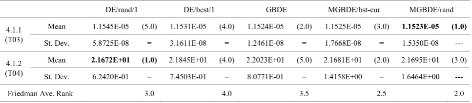
The results obtained by DE/rand/1, DE/best/1, GBDE, MGBDE/bst-cur and MGBDE/rand are summarized in Table 1 in terms of solution accuracy (the mean of the best-of-run values for 25 runs). Table 1 also uses the Friedman test [10] to compare the performance of multiple algorithms on the selected control problems. The Friedman test ranks the algorithms for each problem separately, the best performing algorithm should have the rank of 1, the second best rank 2, etc. In case of ties, average ranks are computed. In the table, the number given in the parentheses represents the corresponding Friedman rank. The last row of Table 1 also shows the Friedman average rank (FAR) of each DE variant. In Table 1, the best rankings are shown in boldface. As can be seen, MGBDE/rand with FAR of 2.0 outperforms MGBDE/bst-cur with FAR of 2.5 The fact reveals that the proposed random-type Gaussian mutation could improve the solution accuracy. MGBDE/rand also performs better than other three DE variants (GBDE, DE/best/1 and DE/rand/1).
In this study, the Wilcoxon’s rank sum test [11] at α = 0.05 is also adopted to evaluate the statistical significance of the results. The comparison results among MGBDE/rand and other algorithms are summarized below the corresponding Friedman rank, where “+”, “-”, and “=” indicate MGBDE/rand is respectively better than, worse than, or similar to the corresponding algorithm according to the Wilcoxon’s rank sum test at α = 0.05. The results reveal that MGBDE/rand does as better as the other four DE variants on the selected two control problems.
According to the Friedman average rank and the Wilcoxon’s rank sum test, it can be seen that the proposed MGBDE/rand outperforms MGBDE/bst-cur, GBDE, DE/best/1 and DE/rand/1.
Table 1. Comparisons of mean the best-of-run solutions
DE/rand/1 DE/best/1 GBDE MGBDE/bst-cur MGBDE/rand
4.1.1 (T03)
Mean 1.1545E-05 (5.0) 1.1531E-05 (4.0) 1.1524E-05 (2.0) 1.1525E-05 (3.0) 1.1523E-05 (1.0) St. Dev. 5.8725E-08 = 3.1611E-08 = 1.2461E-08 = 1.7668E-08 = 1.5350E-08 ---
4.1.2 (T04)
Mean 2.1672E+01 (1.0) 2.1845E+01 (4.0) 2.2023E+01 (5.0) 2.1681E+01 (2.0) 2.1695E+01 (3.0) St. Dev. 6.2420E-01 = 7.4503E-01 = 8.0771E-01 = 1.4158E+00 = 1.6464E+00 ---
[image:4.595.65.549.602.708.2]5. Conclusions
Inspired by DE/rand/1 and GBDE, this study proposed the so-called rand-type Gaussian mutation strategy to improve the search performance of MGBDE. The proposed Gaussian mutation strategy is also parameter free. This study uses the Friedman test and the Wilcoxon’s signed rank test at α = 0.05 to compare the performance of multiple algorithms on two real-world optimal control problems given in IEEE - CEC 2011 evolutionary algorithm competition, viz., the bifunctional catalyst blend optimal control problem and the optimal control of a nonlinear stirred tank reactor,. Simulation results show that MGBDE/rand outperforms MGBDE/bst-cur, DE/rand/1, DE/best/1, and GBDE in terms of solution accuracy.
Acknowledgements
This work was supported by the Ministry of Science and Technology, Taiwan, under Grant MOST 104-2221-E- 262-009.
REFERENCES
[1] R. Storn, K. Price. Differential evolution – a simple and efficient heuristic for global optimization over continuous space, J. Global Optim., Vol. 11, No. 4, 341-359, 1997. [2] X. F. Lu, K. Tang, B. Sendhoff, X. Yao. A new
self-adaptation scheme for differential evolution. Neurocomputing, Vol. 146, 2-16, 2014.
[3] J. Zhang, A. C. Sanderson. JADE: adaptive differential evolution with optional external archive, IEEE Trans. Evol. Comput., Vol. 13, No. 5, 945-958, 2009.
[4] S. M. Islam, S. Das, S. Ghosh, S. Roy, P. N. Suganthan, An adaptive differential evolution algorithm with novel mutation and crossover strategies for global numerical optimization, IEEE Trans. Syst., Man, Cybern.: B, Vol. 42,
No. 2, 482-500, 2012.
[5] J. Brest, S. Greiner, B. Bošković, M. Mernik, V. Žumer. Self-adapting control parameters in differential evolution: a comparative study on numerical benchmark problems, IEEE Trans. Evol. Comput., Vol. 10, No. 6, 646-657, 2006. [6] M. G. H. Omran, A. P. Engelbrecht, A. Salman. Bare bones
differential evolution, Eur. J. Oper. Res., Vol. 196, No. , 128-139, 2009.
[7] H. Wang, S. Rahnamayan, H. Sun, M. G. M. Omran. Gaussian bare-bones differential evolution, IEEE Trans. Cybern., Vol. 43, No. 2, 634-647, 2013.
[8] W. Gong, Z. Cai, X. Ling, H. Li. Enhanced differential evolution with adaptive strategies for numerical optimization, IEEE Trans. Syst., Man, Cybern.: B, Vol. 41, No. 2, 397-413, 2011.
[9] S. Das and P. N. Suganthan. Problem Definitions and Evaluation Criteria for CEC 2011 Competition on Testing Evolutionary Algorithms on Real World Optimization Problems, Nanyang Technol. Univ., Singapore, Tech. Rep., 2010.
[10]S. Garcia, A. Fernandez, J. Luengo, and F. Herrera, Advanced nonparametric tests for multiple comparisons in the design of experiments in computational intelligence and data mining: Experimental analysis of power, Information Science 180 (10) (2010) 2044-2064.
[11]J. Derrac, S. Garc´ıa, D. Molina, F. Herrera, A practical tutorial on the use of nonparametric statistical tests as a methodology for comparing evolutionary and swarm intelligence algorithms, Swarm and Evolutionary Computation 1 (1) (2011) 3-18.
[12]R. Luus, B. Bojkov. Global optimization of the bifunctional catalyst problem, Can. J. Chem. Eng., Vol. 72, 160-163, 1994.
[13]R. Luus. Iterative Dynamic Programming, Chapman & Hall/CRC Press, Boca Raton, FL, 2000.