Transfer Learning For Message Passing Algorithm

(1)

International Journal of Emerging Technology and Advanced Engineering

Website: www.ijetae.com (ISSN 2250-2459,ISO 9001:2008 Certified Journal, Volume 3, Issue 6, June 2013)

443

Transfer Learning For Message Passing Algorithm

Kanchan Govila

1

, Shailendra Shrivastava

2

1_{[email protected]} 2_{[email protected]}

Abstract— A new learning scenario, Transfer Learning (TL) has improves learning performance when the data can be in different feature spaces and where no correspondence between data instances in these spaces is provided. Transfer learning has been used to present image clustering as an example to illustrate how unsupervised learning can be improved by transferring knowledge from auxiliary data. This paper proposes a new and far more efficient method of Transfer Learning for Message Passing Algorithm. Based on this they cluster a small collection of images using readily available annotated image data so as to improve the speed and performance of clustering and also to measure the quality of our clustering results. Message Passing was recently introduced as an unsupervised learning algorithm for exemplar based clustering. It operates by simultaneously considering all data point as potential exemplars and exchanging messages between data points until a good set of exemplars and clusters emerges. This Algorithm improves the speed and performance of our clustering. Speed and Performance is measured in terms of Entropy and F-measure.

Keywords— Transfer Learning, Message Passing Algorithm, Entropy, F-measure.

I. INTRODUCTION

Machine learning usually refers to the changes in systems that perform tasks associated with artificial intelligence (AI). Such tasks involve recognition, diagnosis, planning, robot control, prediction, etc. The changes might be either enhancement to already performing systems or as initio synthesis of new systems. Machine learning is a branch of artificial intelligence, is a scientific discipline that is concerned with the design and development of algorithms that allow computers to evolve behaviors based on empirical data, such as from sensor data or databases[1]. Data mining and machine learning technologies have already achieved significant success in many knowledge engineering areas including classification, regression and clustering. However, many machine learning methods work well only under a common assumption: the training and test data are drawn from the same feature space and the same distribution. When the distribution changes, most statistical models need to be rebuilt from scratch using newly collected training data. In many real world applications, it is expensive or impossible to recollect the needed training data and rebuild the models. It would be nice to reduce the need and effort to recollect the training data.

In such cases, knowledge transfer or transfer learning between task domains would be desirable and which allows the domains, tasks, and distributions used in training and testing to be different [2].

The need for transfer learning may arise when the data can be easily outdated. In this case, the labeled data obtained in one time period may not follow the same distribution in a later time period. In the real world, we observe many examples of transfer learning. For example, we may find that learning to recognize apples might help to recognize pears. Similarly, learning to play the electronic organ may help facilitate learning the piano [2].

II.

B

ACKGROUND

The study of Transfer learning is motivated by the fact that people can intelligently apply knowledge learned previously to solve new problems faster or with better solutions. The fundamental motivation For Transfer learning in the field of machine learning was discussed in a NIPS-95 workshop on ―Learning to Learn‖, which focused on the need for lifelong machine-learning methods that retain and reuse previously learned knowledge. Research on transfer learning has attracted more and more attention since 1995 in different names: learning to learn, life-long learning, knowledge transfer, inductive transfer, multi-task learning, knowledge consolidation, context sensitive learning, knowledge-based inductive bias, Meta learning, and incremental/cumulative learning. Among these, a closely related learning technique to transfer learning is the multi-task learning framework which tries to learn multiple tasks simultaneously even when they are different. A typical approach for multi-task learning is to uncover the common (latent) features that can benefit each individual task [3]. In 2005, the Broad Agency Announcement (BAA) 05-29 of Defense Advanced Research Projects Agency (DARPA)‘s, Information Processing Technology Office (IPTO) gave a new mission of transfer learning: the ability of a system to recognize and apply knowledge and skills learned in previous tasks to novel tasks. In this definition,

(2)

International Journal of Emerging Technology and Advanced Engineering

444

The roles of the source and target tasks are no longer symmetric in transfer learning.

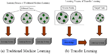
[image:2.612.54.268.268.373.2]

Figure 1 shows the difference between the learning Processes of traditional and transfer learning techniques. As we can see, traditional machine learning techniques try to learn each task from scratch, while transfer learning techniques try to transfer the knowledge from some previous tasks to a target task when the latter has fewer high-quality training data.

Figure 1: Different Learning Processes between Traditional Machine Learning and Transfer Learning

In transfer learning, we have the following three main research issues:

(1) What to transfer. (2) How to transfer. (3) When to transfer.

―What to transfer‖ asks which part of knowledge can be transferred across domains or tasks. Some knowledge is specific for individual domains or tasks, and some knowledge may be common between different domains such that they may help improve performance for the target domain or task.

After discovering which knowledge can be transferred, learning algorithms need to be developed to transfer the knowledge, which corresponds to the ―how to transfer‖ issue.

―When to transfer‖ asks in which situations, transferring skills should be done. Likewise, we are interested in knowing in which situations, knowledge should not be transferred. In some situations, when the source domain and target domain are not related to each other, brute-force transfer may be unsuccessful.

Transfer learning is categorizing under three sub-settings: (1) Inductive Transfer Learning

(2) Transductive Transfer Learning (3) Unsupervised Transfer Learning

In the inductive transfer learning setting, the target task is different from the source task, no matter when the source and target domains are the same or not. It is further categorized into two cases:

(a) A lot of labeled data in the source domain are available.

(b) No labeled data in the source domain are available.

In the Transductive transfer learning setting, the source and target tasks are the same, while the source and target domains are different. It is further categorized into two cases:

(a) The feature spaces between the source and target domains are different,

(b) The feature spaces between domains are the same.

Finally, in the unsupervised transfer learning setting, Similar to inductive transfer learning setting, the target task is different from but related to the source task. In this case, there are no labeled data available in both source and target domains in training.

A. Problem Statement

(3)

International Journal of Emerging Technology and Advanced Engineering

445

III.

L

ITERATURE

S

URVEY

Although many proposals have been published in the last few years, there are still lots of open issues related to Transfer Learning. Different approaches have been proposed trying to enhance the speed and performance of transfer learning in classification and clustering problem many aspects as we see in our discussion

.

A. Heterogeneous Transfer Learning Between Languages

This previous work is based on cross-language classification as an example of heterogeneous transfer learning. This example is related to our image clustering problem because they both rely on data from different feature spaces.

As the World Wide Web in China grows rapidly, it has become an increasingly important problem to be able to accurately classify Chinese Web pages. However, because the labeled Chinese Web pages are still not sufficient, we often find it difficult to achieve high accuracy by applying traditional machine learning algorithms to the Chinese Web pages directly. In this problem we have given a collection of labeled English documents and a large number of unlabeled Chinese documents. The English and Chinese Texts are not aligned. Our objective is to classify the Chinese documents into the same label Space as the English data.

The key observation is that even though the data use different text features, they may still share many of the same semantic information. What they need to do is to uncover this latent semantic information by finding out what is common among them. They did this in [6] by using the information bottleneck theory [7]. In their work, they first translated the Chinese document into English automatically using some available translation software, such as Google translate. Then, they encoded the training text as well as the translated target text together, in terms of the information theory. They allowed all the information to be put through a ‗bottleneck‘ and be represented by a limited number of code-

words

(i.e. labels in the

classification problem).

Finally, information bottleneck was used to maintain most of the common information between the two data sources, and discard the remaining irrelevant information. In this way, they can approximate the ideal situation where similar training and translated test pages shared in the common part are encoded into the same codewords, and are thus assigned the correct labels.

In [6], they experimentally showed that heterogeneous transfer learning can indeed improve the performance of cross-language text classification as compared to directly training learning models (e.g., Naïve Bayes or SVM) and testing on the translated texts.

B. Heterogeneous Transfer Learning for Image clustering via social web

This work makes use of PLSA. Probabilistic latent semantic analysis (PLSA) is a widely used Probabilistic model [8], and could be considered as a probabilistic implementation of latent semantic analysis (LSA) [9]. An extension to PLSA was proposed in [10], which incorporated the hyperlink connectivity in the PLSA model by using a joint probabilistic model for connectivity and content. Moreover, PLSA has shown a lot of applications ranging from text clustering [11] to image analysis [12]. They present our annotation-based probabilistic latent semantic analysis algorithm (aPLSA), which extends the traditional PLSA model by incorporating annotated auxiliary image data. Intuitively, our algorithm aPLSA

performs PLSA analysis on the target images, which are converted to an image instance-to-feature co-occurrence matrix. At the same time, PLSA is also applied to the annotated image data from socialWeb, which is converted into a text-to-image featureco -occurrence matrix. In order to unify those two separate PLSA models, these two steps are done simultaneously with common latent variablesused as a bridge linking them. Through these common latent variables, which are now constrained by both target image data and auxiliary annotation data, a better clustering result is expected for the target data. This is done by first learning the high-quality latent variables in the auxiliary data and then transferring this knowledge to help improve the clustering of the target image data. They conducted experiments on two image data sets, using the Flickr data as the annotated auxiliary image data, and showed that our

aPLSA algorithm can greatly outperform several state-of-the-art clustering algorithms [17].

C. Other Works in Transfer Learning

In the past, several other works made use of transfer learning for cross-feature-space learning. To handle the cross language learning problem by translating the data into a same language and applying kNN on the latent topic space for classification. Most learning algorithms for dealing with cross-language heterogeneous data require a

(4)

International Journal of Emerging Technology and Advanced Engineering

446

For those data that are in different feature spaces where no translator is available, a Markov-logic-based transfer learning algorithm, which is called deep transfer, for transferring knowledge between biological domains and Web domains.[13] proposed a novel learning paradigm, known as translated learning, to deal with the problem of learning heterogeneous data that belong to quite different feature spaces by using a risk minimization framework.

D. Relation to Clustering

Compared to many previous works on image clustering, we note that traditional image clustering is generally based on techniques such as Kmeans [14] and hierarchical clustering. However, when the data are sparse, traditional clustering algorithms may have difficulties in obtaining high-quality image clusters. Recently, several researchers have investigated how to leverage the auxiliary information to improve target clustering performance, such as supervised clustering, semi-supervised clustering, self-taught clustering [15], etc.

IV.

P

ROPOSED

T

ECHNIQUES

Clustering is the task of assigning a set of objects into groups (called clusters) so that the objects in the same cluster are more similar (in some sense or another) to each other than to those in other clusters. Clustering is a main task of explorative data mining, and a common technique for statistical data analysis used in many fields, including machine learning, pattern recognition, image analysis, information retrieval, and bioinformatics. There are many Clustering algorithms such as partitioning and hierarchical Clustering algorithms. Partitional algorithms typically run multiple times with different starting states, and the best configuration obtained from all of the runs is used as the output clustering [16].The k- means is the simplest and most commonly used algorithm One of the main disadvantages to k-means is the fact that you must specify the number of clusters as an input to the algorithm. As designed, the algorithm is not capable of determining the appropriate number of clusters and depends upon the user to identify this in advance.

Exemplar based technique k-medoids algorithm works well only when the number of clusters is small and chances are good that at least one restart lies close to a good clustering solution. Message Passing is the new clustering algorithm, which is based on the similarity matrix between pairs of data points and messages are exchanged between data points until clustering results emerges.

Performance of Message Passing can be improved by increasing the similarity, adjusting the preference and damping factor parameter.

A. Description of Message Passing Algorithm

Affinity propagation simultaneously considers all data points as possible exemplars, exchanging real-valued messages between them until a high quality set of exemplars (and corresponding clusters) emerges. Messages are updated on the basis of simple formulae that reflect sum product or max-product update rules and, at any point in time, the magnitude in each message reflects the current affinity that one point has for choosing another data point as its exemplar, hence the name ―affinity propagation‖. Affinity propagation takes as input a collection of real-valued similarities between data points, {s(i, k)}, where each similarity s(i, k) indicates how well the data point with index k is suited to be the exemplar for data point i.[18]

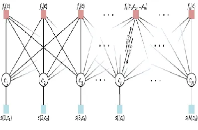
B. Factor Graph

A factor graph is a bipartite graph that expresses the structure of the factorization. A factor graph has a variable node for each variable xi, a factor node for each local

function fi, and an edge connecting variable node xi to

[image:4.612.330.529.489.620.2]

factor node fi if and only if xi is an argument of fi.

Figure 2: Affinity Propagation On Factor Graph

(5)

International Journal of Emerging Technology and Advanced Engineering

447

When the goal is to minimize squared error, each similarity is set to a negative squared error (Euclidean distance):

[image:5.612.334.530.140.283.2]

For points xi and xk,

s(i,k) = −||xi − xk||².

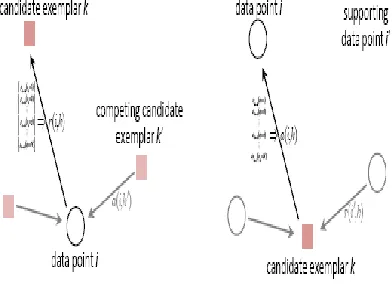
There are two kinds of message exchanged between data points, and each takes into account a different kind of competition. Messages can be combined at any stage to decide which points are exemplars and, for every other point, which exemplar it belongs to. The ―responsibility‖ r(i,k), sent from data point i to candidate exemplar point k, reflects the accumulated evidence for how well-suited point k is to serve as the exemplar for point i, taking into account other potential exemplars for point i (Figure 2.13). The ―availability‖ a(i,k), sent from candidate exemplar point k to point i, reflects the accumulated evidence for how appropriate it would be for point i to choose point k as its exemplar, taking into account the support from other points that point k should be an exemplar. r(i,k) and a(i,k) can be viewed as log-probability ratios. To begin with, the availabilities are

initialized to zero: a(i,k) = 0. Then, the

responsibilities are computed using the rule:

r(i,k)← s(i,k) – max

k‘ s.t. k′ ≠k

{a(i,k′)+s(i,k′)}

Whereas the above responsibility update lets all candidate exemplars compete for ownership of a data point, the following availability update gathers evidence from data points as to whether each candidate exemplar would make a good exemplar:

a(i,k) ← min{ 0,r(k,k) + ∑i′s.t. i′є max {0,r(i′,k)}}

The availability a (i, k) is set to the self responsibility r(k,k) plus the sum of the positive responsibilities candidate exemplar k receives from other points. If the self responsibility r(k,k) is negative (indicating that point k is currently better suited as belonging to another exemplar rather than being an exemplar itself), the availability of point k as an exemplar can be increased if some other points have positive responsibilities for point k being their exemplar.[18]

Figure 3: Responsibilities and Availabilities Messages

At any point during affinity propagation, availabilities and responsibilities can be combined to identify exemplars. For point i, the value of k that maximizes a(i,k) + r(i,k) either identifies data point that is the exemplar for point i. The message-passing procedure may be terminated after a fixed number of iterations, after changes in the messages fall below a threshold, or after the local decisions stay constant for some number of iterations point i as an exemplar if k = i, or identifies the data point that is the exemplar for point i. each iteration of affinity propagation consisted of -

(

i) Updating all responsibilities given the availabilities, (ii) Updating all availabilities given the responsibilities, and

(iii) Combining availabilities and responsibilities to monitor the exemplar decisions and terminate the algorithm when these decisions did not change for 10 iterations.[18]

C. Preferences For Affinity Propagation

(6)

International Journal of Emerging Technology and Advanced Engineering

448

A good initial choice for the preference is the minimum similarity or the median similarity.[19]

D. Advantages of Affinity Propagation

(1) Affinity propagation is a low error, high speed, flexible, and an easy-to-code clustering algorithm that identifies clusters, exemplars, and outliers.

(2) Affinity propagation‘s ability to operate on the basis of nonstandard optimization criteria makes it suitable for exploratory data analysis using unusual measures of similarity. Unlike metric space clustering techniques such as k-means clustering.

(3) Affinity propagation can be applied to problems where the data do not lie in a continuous space.

(4) Affinity propagation can be applied to problems where the similarities are not symmetric [i.e., s(i,k) ≠ s(k,i)] and to problems where the similarities do not satisfy the triangle inequality [i.e., s(i,k) < s(i, j) + s( j,k)].

(5) Affinity propagation is deterministic, i.e., its clustering results do not depend on initialization, unlike most clustering methods such as k-means.

(6) Affinity propagation is a fast clustering algorithm especially in the case of large number of clusters and has some advantages: speed, general applicability and good performance.

E. Steps of Message Passing Algorithm

In the proposed algorithm, we are constructing clustering solution using Message Passing. Which commences by considering all the data items as potential exemplars, and then recursively transmits real valued messages along edges of a network whose nodes are data items. In the proposed algorithm, firstly the exemplars are returned from text message passing clustering, through these exemplars similarity matrix between these exemplars points is set to the highest value. Then again message passing clustering is applied to images data points.

This process repeated for the fixed number of iteration, after changes in the messages fall below a threshold, or after the local decision stays constant for some number of iterations In the Message Passing algorithm each iteration involves the following steps:

1) Updating all the responsibilities given the availabilities. 2) Updating all availabilities given the responsibilities. 3) Combining availabilities and responsibilities to monitor the exemplar decisions and terminate the algorithm when these decisions did not change.

Similarities s(i,k) indicates how well the data point with index k is suited to be the exemplar for data point i. If the data are real-valued, a common choice for similarity is negative Euclidean distance. For points xi and xk ,

s(i,k) = -||xi – xk||2.

The preference of point i, called p(i) or s(i,i), is the a priori suitability of point i to serve as an exemplar. Preferences can be set to a global (shared) value, or customized for particular data points. High values of the preferences will cause affinity propagation to find many exemplars (clusters), while low values will lead to a small number of exemplars (clusters). A good initial choice for the preference is the minimum similarity or the median similarity.

Algorithm:

Input: Similarity Matrix and Preference;

Output: Clustering Solution;

Step 1: Construct the similarity Matrix based on the negative Euclidean distance for feature vectors of text.

Step 2: Calculate the Preference

(7)

International Journal of Emerging Technology and Advanced Engineering

449

Step 3: The responsibility message r(i,k) sent from data point i to k is to serve as the exemplar for the data point i. Responsibilities are calculated as follows:

r(i,k)← s(i,k) – maxk‘ s.t. k′ ≠k{a(i,k′)+s(i,k′)}

In the first iteration, because the availabilities are zero, r(i,k) is set to the input similarity between point i and point k as its exemplar, minus the largest of the similarities between point i and other candidate exemplars.

The responsibility r(k,k) ―self-responsibility‖ is set to the input preference that point k be chosen as an exemplar, s(k,k), minus the largest of the similarities between point i and all other candidate exemplars.

Step 4: The availability message a(i,k) sent from candidate exemplar point k to i reflects the accumulated evidence for how appropriate it would be for point i to choose point k as its exemplar.

Availabilities are calculated as follows: a(i,k) ← min{ 0,r(k,k) + ∑i′s.t. i′є max {0,r(i′,k) }}

The ―self-availability‖ a(k,k) is updates as

a(k,k) ← ∑ i′s.t.i′≠k max {0,r(i′,k)}

This message reflects accumulated evidence that point k is an exemplar, based on the positive responsibilities sent to candidate exemplar k from other points.

Step 5: Set damping factor, convergence iteration and maximum iteration.

Damping factor (dampfact): When updating the messages, it is important that they be damped to avoid numerical oscillations that arise in some circumstances.

Msgnew = (dampfact)(msgold) + (1- dampfact)(msgnew)

Convits and maxits: Affinity propagation iteratively computes responsibilities and availabilities.

The algorithm terminates if decisions for the exemplars and the cluster boundaries are unchanged for convits iterations, or if maxits iterations are reached.

Step 6: At any point during proposed algorithm availabilities and responsibilities can be combined to identify exemplars. For point i, the value of k that maximizes a(i,k) + r(i,k) either identifies point i as an exemplar if k = i, or identifies the data point that is the exemplar for point i.

Step 7: Again calculate the similarity matrix for image data points, based on the negative Euclidean distance for feature vectors of image.

Step 8: Calculate the Preference.

Step 9: Only the identified exemplars are set to their highest value in the above similarity matrix.

Step 10: repeat step 3 to 7 for the similarity matrix obtained in step 10 and preference in step 9. The algorithm is halted after a fixed number

of iterations or after the

exemplars do not change for a given number of

iterations.

Stop

V. PERFORMANCE EVALUATION

We now analyze the effectiveness of our Message Passing algorithm. Because, to our best of knowledge, few existing methods addressed the problem of image clustering with the help of social

Annotation image data, we can only compare our Message Passing Algorithm with several state-of-the-art clustering algorithms that are not directly designed for our problem. The first baseline is the well-known Kmeans algorithm [14].

For this we have two strategies:

(1) Separated Phase: the baseline method was applied on the target image data only;

(8)

International Journal of Emerging Technology and Advanced Engineering

450 A. MATLAB Setup

MATLAB (matrix laboratory) is a numerical computing environment and fourth-generation programming language. Developed by Math Works, MATLAB allows matrix manipulations, plotting of functions and data, implementation of algorithms, creation of user interfaces, and interfacing with programs written in other languages, including C, C++, Java, and FORTRAN.

Although MATLAB is intended primarily for numerical computing, an optional toolbox uses the MuPAD symbolic engine, allowing access to symbolic computing capabilities. An additional package, Simulink, adds graphical multi-domain simulation and Model-Based Design for dynamic and embedded systems.

In the research work, we have evaluated accuracy, entropy of the proposed algorithm. To measure these performance parameters we have used 50 data sets from Caltech- 256.

B. Description of Dataset

Here, experiment is done on 256. The Caltech-256 dataset has Caltech-256 image objective categories, ranging from animals to buildings, from plants to automobiles, etc, Annotations is also done over these categories.

Out of 256 categories I have taken 50 different categories in my experiment for transfer learning by Message Passing which is done in two phases:

1) Separate Phase 2) Combined Phase

In separate phase Message Passing Algorithm is applied only on image set. Where as in combined phase message passing is applied on both annotation as well as on image set. In my experiment I have calculated feature Vectors of both text and image dataset. For text feature extraction, I have used Vector Space Model (VSD).

C. Performance Parameter

We measure the performance of our algorithm in the form of following parameters

:

F-measure: F-measure is a measure of a test's accuracy. It considers both theprecisionpand therecallrof the test to compute the score:pis the number of correct results divided by the number of all returned results andris the number of correct results divided by the number of results that should have been returned.

F-measure = 2. Precision * recall/Precision + recall

Entropy:

Entropy is a measure of the uncertainty associated with a random variable. In our problem, entropy serves as a measure of randomness of clustering result. Lower entropy indicates less randomness and thus better clustering results.

Entropy = -sum (p.*log2(p)) D. Result Analysis

Result Analysis is done between Kmeans Algorithm and the Message Passing Algorithm for Transfer Learning:

Dataset (each at 90%)

Kmeans Algorithm Message Passing Algorithm

Separate

Combined

Separate

Combined

Entropy F-measure Entropy F-measure Entropy F-measure Entropy F-measure

1

3.4343 12 2.7411 15.6923 3.3611 18 1.4395 60

2

4.1686 14.2326 1.6233 18 3.3601 17.4857 0.5451 20.9286

(9)

International Journal of Emerging Technology and Advanced Engineering

451

4

4.3745 20.4000 1.6673 20.0000 4.1254 20.889 0.7546 34.1818

5

3.7337 14.2326 2.5295 14.8571 3.1446 11.3684 1.1974 46.6667

6 3.6382

11.7692

1.9195

10.9333

3.0591

17.1765

2.2549

146

7 3.6675

11.4783

2.0840

11.5152

2.6343

10.5600

0.7846

21.2500

8 3.5690

12.2424

2.6777

21.2500

3.2495

14.9630

0.5950

6.8475

9 4.2071

15.5385

3.0230

20.889 3.6017

13.2308

1.5476

24.5714

10 3.7552

8.5957

1.6982

10.9091

3.6488

9.8182

2.3625

54

VI.

C

ONCLUSION

&

F

UTURE

P

ROSPECTIVES

In the proposed algorithm I tried to improve the solution quality of clusters which are produced by method called Affinity Propagation. By the experimental result, it is observed that the proposed algorithm gives 100 % accuracy for datasets which is measured by the parameter called F-measure and lower value of entropy. From the experimental result on the dataset shows that the Message Passing algorithm serves a good clustering algorithm which identifies exemplars quickly. Finally it is concluded from the results that the Message

Passing

algorithm is a good

clustering algorithm that generates an efficient clustering solution

Some possible future work may include: Transfer learning can also be used for audio and video data. I am also interested to use this algorithm in applications where n-wise similarities are useful and for the sparse data where many data points cannot be represented by many others as exemplars: i.e. s(i,k) = -∞. In natural Language processing, there are many future opportunities to transfer learning.

REFERENCES

[1] Nils J.Nilson, Introduction to Machine Learning, Robotics Laboratory. Department Of Computer science Stanford University CA 94305 Nov.1998.

[2] Sinno Jialin Pan and Qiang Yang, ―A survey On Transfer Learning, Transaction On Knowledge and Data Engineering‖,vol.22 No.10, Oct.2010.

[3] R. Caruana, ―Multitask learning,‖ Machine Learning, vol. 28(1), pp. 41–75, 1997.

[4] R. Raina, A. Battle, H. Lee, B. Packer, and A. Y. Ng, ―Self-taught learning: Transfer learning from unlabeled data,‖ in Proceedings of the 24th International Conference on Machine Learning, Corvalis, Oregon,USA, pp. 759–766 , June 2007.

[5] W. Dai, Q. Yang, G. Xue, and Y. Yu, ―Self-taught clustering,‖ in Proceedings of the 25th International Conference of Machine Learning.ACM, pp. 200–207, July 2008.

[6] X. Ling, G.-R. Xue, W. Dai, Y. Jiang, Q. Yang, and Y. Yu, ―Can chinese web pages be classified with English data source?‖ in Proceedings of the 17th International Conference on World Wide Web. Beijing, China: ACM, pp. 969–978, April 2008.

[7] Naftali Tishby,Fernando C.Pereira, and William Bialek.‖The Information Bottleneck Method.‖.In proc.of the 37th_Annual

Allerton Conference on Communication, Control and Computing, pp.368-377, 1999.

[8] Thomas Hofmann, ―Probabilistic latent semantic analysis‖. In Proc. Of Uncertainty in Artificial Intelligence,UAI99.pp 289-296,1999. [9] Scott Deerwester,Susan T.Dumais, George W.Furnas, Thomas

K.L,and Richard Harshman. ―Indexing by latent semantic analysis‖.Journal of the American Society for Information Science,pp 391-407,1990

(10)

International Journal of Emerging Technology and Advanced Engineering

452

[11] Thomas Hofmann.‖Unsupervised learning by probabilistic latent semantic analysis‖.Machine learning.volume 42,number 1-2,Kluwer Academic Publishers,pp 177-196,2001.

[12] J.Sivic,B.C. Russell, A.A.Efros,A.Zisserman, and W.T. Freeman,‖Discovering object categories in image collections,In ICCv,2005.

[13] Wenyuan Dai, Yuqiang Chen, Gui-Rong Xue, Qiang Yang, and Yong Yu. ―Translated learning: Transfer learning across different feature spaces.‖ In NIPS, pp 353–360,2008

[14] J. B. MacQueen.‖ Some methods for classification and analysis of multivariate observations.‖ In Proceedings of Fifth Berkeley Symposium on Mathematical Statistics and Probability, Berkeley, CA, USA, pp1:281–297,1967.

[15] Wenyuan Dai, Qiang Yang, Gui-Rong Xue, and Yong Yu. ―Self-taught clustering.‖ In ICML , pp 200–207. Omnipress.2008. [16] Jain, A. K., Murthy, M. N., & Flynn, P. J. Data clustering: A

review. ACMComputing Surveys, 31(3), 264-323, 1999. [17] Yuqiang Chen,Gui-rong Xue, Wenyuan Dai, Yong Yu,

―Heterogeneous Transfer Learning For Image Clustering via the Social Web‖in proceedings of the 47th_{annual meeting of the ACL}

and the 4th_{IJCNLP of the AFNLP,pages 1-9,Suntec, Singapore,2-7}

August 2009.

[18] Frey, B. J. & Dueck, D. Clustering by passing messages between data points. Science, 305(5814), 972 – 976, 2007.