Stability Analysis of Wang's Stretching/ Shrinking Sheet Problem for Nanofluids

(1)

Stability

Analysis

of

Wang

'

s

Stretching/

Shrinking

Sheet

Problem

for

Nanofluids

Mohamad Mustaqim Junoh

1,∗

,

Fadzilah Md Ali

1,2

_,

_{Norihan Md Arifin}

1,2

_,

_{Norfifah Bachok}

1,2

1_{Institute for Mathematical Research, Universiti Putra Malaysia, 43400 UPM Serdang, Selangor, Malaysia} 2_{Department of Mathematics, Faculty of Science, Universiti Putra Malaysia, 43400 UPM Serdang, Selangor, Malaysia}

∗_{Corresponding Author: [email protected]}

Received July 11, 2019; Revised August 25, 2019; Accepted September 02, 2019

Abstract

The steady stagnation-point flow of nanofluid over a stretching or shrinking sheet in its own plane is inves-tigated. The governing nonlinear partial differential equations are transformed into a nonlinear ordinary differential equations via the similarity transformation before they are solved numer-ically using the bvp4c solver in the MATLAB. Three different types of nanoparticles(Cu, Al2O3, T iO2)in the water-based fluid are analyzed in this paper. Effects of the solid volume fraction φ on the fluid flow and heat transfer are evaluated. Numerical results are obtained for velocity and temperature distribution, as well as the skin friction coefficientf00(0)and local Nusselt number−θ0(0)are presented graphically. There exist dual solutions for a certain range of stretching/shrinking parameter . Therefore, a stability analysis is performed to determine which solution is linearly stable and physically realizable. From the stability analysis it is found that the first solution is stable whilst the second solution is not.

Keywords

Boundary Layer, Dual Solutions, Stagnation-point Flow, Nanoparticles, Stability Analysis

1 Introduction

The number of researchers that discover and examine the fluid flow and heat transfer over a stretching or shrinking sheet problem has been tremendously expended in recent years. The increase in number of researches in this field has been encour-aged by the large diversity of real-world applications especially in engineering procedures and productions. In the theory of fluid dynamics, stagnation point flow is the fluid motion near the stagnation region where it exists at the surface of objects in the flow. Hiemenz [1] was the pioneer in stagnation point flow problem. He used a similarity transformation to reduce the Navier-Stokes equations to a nonlinear ordinary differen-tial equation, solving the two-dimensional stagnation flow to-wards a stationary plate problem. Miklavˇciˇc and Wang [2]

were the first investigated the flow due to a shrinking sheet. They reported that the boundary layer flow over a shrinking sheet is presence in two conditions which are imposing an ad-equate suction on the boundary and by considering stagnation flow. On the other hand, the combination of both stagnation point flow and shrinking sheet was considered by Wang [3]. He found that the shrinking sheet has many unique character-istics such as for a larger shrinking rates, the solution does not exist. Therefore, the study of fluid flow over a stretch-ing/shrinking sheet has been explored by a substantial amount of researchers under different physical conditions. Recently, pioneering efforts on the flow over a stagnation point towards a stretching/shrinking sheet from the past researchers have spark interest to many new researchers. This present study has set a purpose to investigate the effects of nanoparticle volume fraction and the heat integration of nanofluids towards stretch-ing/shrinking sheet. This present work is remotely extending the past work done by Ali et al. [4]. Prior to the work, Ali et al. [4] had done a study on the steady stagnation-point flow of a viscous and incompressible fluid over a continuously stretch-ing or shrinkstretch-ing sheet in its own plane in a water-based copper

(Cu)nanofluid using shooting method technique. Solving this problem has resulted in dual-solutions. Therefore, a stability analysis is carried out to determine either the first or second solution is practically acceptable. The stability analysis in this study is done by following the works of [5-9].

2 Mathematical Formulation

Take into consideration the steady stagnation-point flow of viscous and incompressible fluid over a stretching or shrinking sheet in its own plane in nanofluid. Following Ali et al. [4] and a model proposed by Tiwari and Das [10], it is presumed that the free stream velocity isue(x) = ax, while the

veloc-ity of the stretching sheet isuw(x) = b(x+c), whereais a

(2)

axis is perpendicular to it. Under these presumptions, the basic equations of this problem can be derived as follows:

∂u ∂x+

∂v

∂y = 0, (1)

u∂u ∂x +v

∂u ∂y =−

1 ρnf ∂p ∂x + µnf ρnf

∂2_u

∂y2, (2) u∂v

∂x +v ∂v ∂y =−

1 ρnf ∂p ∂y + µnf ρnf

∂2v

∂y2, (3) u∂T

∂x +v ∂T

∂y =αnf ∂2_T

∂y2. (4)

Following Khanafer et al. [11] and Oztop and Abu-Nada [12] we employ

µnf =

µf

(1−φ)2.5, αnf =

knf

(ρCp)nf

,

ρnf = (1−φ)ρf+φρs,

(ρCp)nf = (1−φ)(ρCp)f+φ(ρCp)s,

knf

kf

=(ks+ 2kf)−2φ(kf−ks) (ks+ 2kf) +φ(kf−ks)

,

(5)

where(ρCp)nf is the heat capacity of the nanofluid. The

dy-namic viscosity of the base fluid µf has been proposed by

Brinkman [13]. Strictly expressions(5)are restricted to spher-ical (or near spherspher-ical) nanoparticles. The boundary conditions of Eqs. (1)–(4) are

u=uw(x) =b(x+c), v= 0, T =Tw at y= 0,

u=ue→ax, T →T∞ as y→ ∞.

(6) Following Wang [3], we presume that Eqs. (1)–(4) subject to the boundary conditions (6) admit the similarity solution

η=

_a

νf

1/2

y, u=axf0(η) +bcg(η),

v=−(aνf)1/2f(η), θ(η) =

T−T∞ Tw−T∞

,

(7)

where primes denote differentiation with respect toη. Using Eq. (3) and the boundary conditions (6), we acquire the fol-lowing expression for the pressurep

p=p0−pnf

a2_x2

2 −µnf

v2

2 +µnf

dv

dy, (8)

wherep0is the stagnation pressure. Thus, we have − 1 ρnf ∂p ∂x = ∂ue ∂t + ∂ue

∂x as y→ ∞. (9)

Subtituting Eqs. (7) and (9) into Eqs. (2)–(4), the following ordinary differential equations are obtained

Af000+f f00−f02+ 1 = 0, (10)

Ag00+f g0−f0g= 0, (11) B 1

P rθ

00

+f θ0 = 0, (12)

where

A= 1

(1−φ)2.5₍₁₋_φ₊_φρ

s/ρf)

,

B = knf/kf

[1−φ+φ(ρCp)s/(ρCp)f]

,

(13)

subject to the new boundary conditions

f(0) = 0, f0(0) =, g(0) = 1, θ(0) = 1

f0(∞)→1, g(∞)→0, θ(∞)→0.

(14)

In the above equations,P ris the Prandtl number andis the velocity ratio parameter defined as

= b

a, (15)

where >0for stretching case and <0for shrinking case. The physical quantities of interest are represented as the skin friction coefficientCfand the local Nusselt numberN ux,

which defined as Cf =

τw

ρfu2e

, N ux=

xqw

kf(Tw−T∞)

, (16)

whereτwis the surface shear stress andqwis the surface heat

flux derived from τw=µnf

_∂u

∂y

y=0

, qw=knf

_∂T

∂y

y=0

. (17)

Using the similarity variables (7), we obtain

CfRe1x/2=

1 (1−φ)2.5

f00(0) + bc

axg

0

(0)

, (18)

N uxRe−1x /2=−

knf

kf

θ0(0), (19)

where the local Reynolds number is represented as Rex =

uex

νf

.

3 Stability Analysis

To carry out the stability analysis, following Merkin [5] and Weidman et al. [6], we take the problem in unsteady case into account. The continuity Eq. (1) holds, while Eqs. (2)–(4) are replaced by

∂u ∂t +u

∂u ∂x+v

∂u ∂y =−

1 ρnf ∂p ∂x+ µnf ρnf

∂2_u

∂y2 (20) ∂v

∂t +u ∂v ∂x+v

∂v ∂y =−

1 ρnf ∂p ∂y+ µnf ρnf

∂2v

∂y2 (21) ∂T

∂t +u ∂T ∂x +v

∂T ∂y =αnf

∂2_T

(3)

wheretdenotes the time. We are now introducing the follow-ing new dimensionless variables:

η=

_a

νf

1/2

y, τ=at,

u=ax∂f

∂η(η, τ) +bcg(η, τ),

v=−(aνf)1/2f(η, τ), θ(η, τ) =

T−T∞ Tw−T∞

(23)

so that Eqs. (20)–(22) can be expressed as

A∂ 3_f

∂η3 −

_∂f

∂η

2

+f∂

2_f

∂η2 + 1− ∂2f

∂η∂τ = 0 (24)

A∂ 2_g

∂η2−f ∂g ∂η −g

∂f ∂η −

∂g

∂τ = 0 (25)

B 1 P r

∂2θ ∂η2 +f

∂θ ∂η −

∂θ

∂τ = 0 (26)

and can be remotely subjected to the boundary conditions

f(0, τ) = 0, ∂f

∂η(0, τ) =, g(0, τ) = 1, θ(0, τ) = 1, ∂f

∂η(η, τ)→1, g(η, τ)→0, θ(η, τ)→0asη→ ∞. (27)

To put the stability of the steady flow solution into a test, f(η) =f0(η),g(η) =g0(η)andθ(η) =θ0(η)satisfying the boundary value problem (10)–(13), we set down

f(η, τ) =f0(η) +e−γτF(η, τ),

g(η, τ) =g0(η) +e−γτG(η, τ),

θ(η, τ) =θ0(η) +e−γτT(η, τ),

(28)

whereγ represents an unknown eigenvalue,F(η, τ),G(η, τ)

andT(η, τ)are small relative tof0(η),g0(η)andθ0(η). Solu-tions of the eigenvalue problem in Eqs. (22)–(25) give an infi-nite set of eigenvalue problemγ1< γ2< ...; ifγ1is negative, there is an initial growth of disturbances and the flow is deemed to be unstable but whenγ1is positive, is an initial decay of dis-turbances and the flow is believe to be stable. Introducing (28) into Eqs. (24)–(27), we get the following linearized problem

A∂ 3_F

∂η3 +f0 ∂2_F

∂η2 +f

00

0F− 2f

0

0−γ

∂F

∂η − ∂2_F

∂η∂τ = 0, (29)

A∂ 2_G

∂η2 −f0 ∂G

∂η −g

0

0F− f

0

0−γ

G−g0 ∂F

∂η − ∂G

∂τ = 0, (30) B∂

2_T

∂η2 +f0 ∂T ∂η +θ

0

0F+γT − ∂T

∂τ = 0, (31) and are subjected to the boundary conditions

F(0, τ) = 0, ∂F

∂η(0, τ) = 0, G(0, τ) = 1, T(0, τ) = 1 ∂F

∂η(η, τ)→0, G(η, τ)→0, T(η, τ)→0asη→ ∞. (32)

The solutions f(η) = f0(η), g(η) = g0(η) andθ(η) = θ0(η)of the steady Eqs. (10)–(14) are gained by settingτ= 0. HenceF(η) = F0(η),G(η) = G0(η)andT(η) = T0(η)in Eqs. (29)–(32) identify initial growth or decay of the solution (28). In this respect, linear eigenvalue problem needs to be solved

AF₀000+f₀00F0+f0F

00

0 − 2f

0

0−γ

F₀0 = 0, (33) AG00₀−f0G

0

0−F0g

0

0−f

0

0G0−F

0

0g0+γG0= 0, (34) B 1

P rT

00

0 +f0T

0

0+θ

0

0F0+γT0= 0, (35) along with the boundary conditions

F0(0) = 0, F

0

0(0) = 0, G0(0) = 0, T0(0) = 0

F₀0(η)→0, G0(η)→0, T0(η)→0 as η→ ∞ (36)

The stability of the steady-state flow solution is based on the smallest eigenvalueγ1. Therefore, the conditionF

0

0(η)→0as η → ∞has been put at rest as suggested by Harris et al. [14] and for a fixed value of eigenvalue,γ. Eqs. (33)–(35) will be solved with the introduction of a new boundary condition that isF000(η) = 1.

4 Results and Discussion

[image:3.595.316.536.594.651.2]

The governing ordinary differential equations (10)–(12), subject to the boundary conditions (14) have been solved nu-merically using bvp4c function in Matlab. The effects of the solid volume fraction of nanofluidφand the Prandtl number P rare examined for three differents nanofluid which are cop-per Cu-water, aluminaAl2O3-water and titania T iO2-water as working fluids. Following Oztop and Abu-Nada [12], the chosen value of the Prandtl numberP ris 6.2 (water) and the value of nanoparticle is from 0 to 0.2(0 ≤φ≤0.2)in which φ = 0 must be compatible with regular fluid. The thermo-physical properties of the base fluid and nanofluid are stated in Table 1.

Table 1.Thermophysical properties of the base fluid and nanoparticles (Oztop and Abu-Nada [12])

Physical Properties

Fluid Phase

(water) Cu Al2O3 T iO2

Cp(J/kgK) 4179 385 765 686.2

ρ(kg/m2) 997.1 8933 3970 4250

k(W/mK) 0.613 400 40 8.9538

(4)

[image:4.595.95.496.104.273.2]

Table 2.Values of the skin friction coefficientf00(0)for some value ofandφforCu−water working fluid

Wang[3]_φ_{= 0} _φ_{= 0} Bachok et al.[15]_φ_{= 0}_.₁ _φ_{= 0}_.₂ _φ_{= 0} _φPresent_{= 0}_.₁ _φ_{= 0}_.₂

2 -1.88731 -1.887307 -2.217106 -2.298822 -1.887307 -2.217106 -2.298822

1 0 0 0 0 0 0 0

0.5 0.71330 0.713295 0.837940 0.868824 0.713295 0.837940 0.868824 0 1.232588 1.232588 1.447977 1.501346 1.232588 1.447977 1.501346 -0.5 1.49567 1.495670 1.757032 1.821791 1.495669 1.757032 1.821791 -1 1.32882 1.328817 1.561022 1.618557 1.328817 1.561022 1.618557

[image:4.595.322.534.309.489.2] [image:4.595.65.275.528.704.2]

[0] [0] [0] [0] [0] [0] [0] -1.15 1.082231 1.082231 1.271347 1.318205 1.082231 1.271347 1.318205

[0.116702] [0.116702] [0.137095] [0.142148] [0.116701] [0.137095] [0.142148] -1.2 0.932473 1.095419 1.135794 0.932473 1.095419 1.135793

[0.233650] [0.274479] [0.284596] [0.233649] [0.274479] [0.284596] 1.2465 0.55430 0.584281 0.686379 0.711679 0.584282 0.686382 0.711680

[0.554297] [0.651161] [0.675159] [0.554295] [0.651157] [0.675157] [ ]indicate second solution.

Figure 1.Velocity profile for various nanoparticles

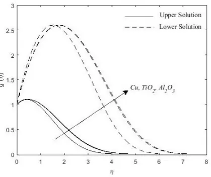
Figure 2.Velocitygprofile for various nanoparticles

The variation of f00(0), g0(0) and −θ0(0) are illustrated in Figures 4–9 for different nanoparticles(Cu, Al2O3, T iO2) and nanoparticle volume fractionφ with stretching/shrinking

Figure 3.Temperature profile for various nanoparticles

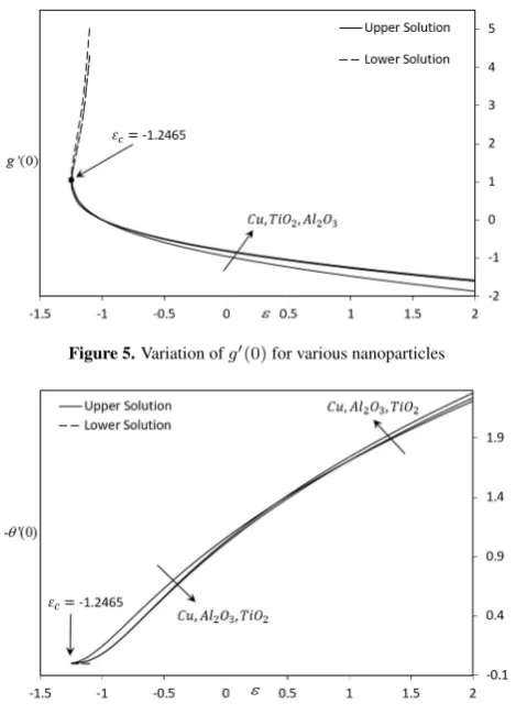
parameter. Based on these figures, for the value > −1

the solutions are unique, dual solutions exist when the value

−1.2465 ≤ ≤ −1 and no solution exist when <

−1.2465 = c, where c is the critical point. This similar

critical point value is also reported by Noor et al. [16] and Awaludin et al. [17]. Notice that from Figures 4 and 7, the value off00(0)is zero when = 1. This due to the fact that when the fluid and solid boundary move with the equal veloc-ity, there is no friction detected on the fluid-solid interface. The skin friction f00(0) and Nusselt number −θ0(0) have higher value forCuthan for Al2O3 andT iO2 as shown in Figures 4 and 6 respectively. This is due to the physical properties of fluid and nanoparticles where the thermal conductivity ofCu is much greater compared toAl2O3andT iO2.

(5)

[image:5.595.51.282.88.236.2] [image:5.595.313.542.91.249.2]

Figure 4.Variation of skin friction coefficient for various nanoparticles

Figure 5.Variation ofg0(0)for various nanoparticles

Figure 6.Variation of local Nusselt number for various nanoparticles

Figure 7.Variation of skin friction coefficient for various value ofφ

[image:5.595.50.285.264.589.2]

Figure 8.Variation ofg0₍₀₎_{for various value of}_φ

[image:5.595.312.543.275.422.2]

Figure 9.Variation of local Nusselt number for various value ofφ

[image:5.595.51.280.613.761.2] [image:5.595.318.536.652.765.2]

Table 3 for several values ofwhen P r = 6.2 andφ = 0.2. From the table, it noticed that the smallest eigenvalueγ1gives a positive value for the first solution and negative value for the second solution. Positive value indicate that is an initial decay of disturbance for the first solution, while the negative value for the second solution showed an initial growth of disturbance. Hence, we can draw a conclusion that only the upper branch solutions are physically significant while the lower branch so-lutions are not. Moreover, it is important to note the eigen values for all nanoparticlesCu,Al2O3andT iO2are the same for the fixed value of.

Table 3.Smallest eigenvaluesγfor different nanofluid with several values of

whenP r= 6.2andφ= 0.2

Nanofluid First Solution Second Solution -1.2 0.57796 -0.51721

Cu -1.24 0.21205 -0.20364 -1.246 0.06216 -0.06142 -1.2 0.57796 -0.51721

Al2O3 -1.24 0.21205 -0.20364

-1.246 0.06216 -0.06142 -1.2 0.57796 -0.51721

T iO2 -1.24 0.21205 -0.20364

(6)

5 Conclusions

A numerical study is performed for the problem of the flow and heat transfer characteristics of a nanofluids

(Cu, Al2O3, T iO2)over a stretching or shrinking sheet in its own plane. Dual solutions are found to be exist for certain ranges values of stretching/shrinking parameter (c < < −1). The stability analysis is done via bvp4c function in MAT-LAB software and their results found that the first solution (up-per branch) is stable and valid physically, while the second so-lution (lower branch) is unstable.

Acknowledgements

The authors gratefully acknowledge the financial re-ceived in the form Geran Putra IPS (Project number: GP-IPS/2018/9570000) from the Universiti Putra Malaysia and MyPhD from the Ministry of Higher Education, Malaysia.

Nomenclature

Roman Letters

a positive constant variable b stretching/shrinking rate variable c stretching origin

Cf skin friction coefficient

Cp specific heat capacity

f(η) dimensionless stream function g(η) dimensionless stream function k thermal conductivity

N ux local Nusselt number

p pressure

p0 stagnation pressure P r Prandtl number qw surface heat flux

Rex local Reynolds number

t time

T temperature of the nanofluid

ue velocity at the edge of the boundary layer

u, v velocity components along thexandydirections, respectively

x, y Cartesian coordinates

Greek Symbols

α thermal diffusivity of the nanofluid γ eigenvalue

γ1 smallest eigenvalue

stretching/shrinking parameter η similarity variable

θ(η) dimensionless temperature µ dynamic viscosity

ν kinematic viscosity

ρ density

τ dimensionless time τw surface shear stress

φ nanoparticle volume fraction

Subscripts

w condition at the surface

∞ condition outside of boundary layer c critical value

f base fluid nf nanofluid s solid fraction

Superscripts

0 _{differentiation with respect to}_η

REFERENCES

[1] K. Hiemenz. Die grenzschicht an einem in den gleichformigen flussigkeitsstrom eingetauchten geraden kreiszylinder. Din-gler’s Polytech J, 326(9), 321–324, 1911.

[2] M. Miklavcic, C. Y. Wang. Viscous flow due to a shrinking shee, Quarterly of Applied Mathematics, 64(2), 283–290, 2006.

[3] C. Y. Wang. Stagnation flow towards a shrinking sheet, Interna-tional Journal of Non-Linear Mechanics, 43(9), 377–382, 2008.

[4] F. M. Ali, R. Nazar, N. M. Arifin, I. Pop. Numerical solutions of Wang’s stretching/shrinking sheet problem for nanofluids, AIP Conference Proceedings, 1557, 330-334, 2013.

[5] J. H. Merkin. On dual solutions occuring in mixed convection in a porous medium, Journal of Engineering Mathematics, 20, 171–179, 1985.

[6] P. D. Weidman, D. G. Kubitschek, A. M. J. Davis. The effect of transpiration on self-similar boundary layer flow over mov-ing surfaces, International Journal of Engineermov-ing Sciences, 44, 730–737, 2006.

[7] S. Mansur, A. Ishak, I. Pop. The magnetohydrodynamic stagna-tion point flow of a nanofluid over a stretching/shrinking sheet with suction, PLOS ONE, Vol.10, No.3, 1–14, 2015.

[8] N. S. M. Adnan, N. M. Arifin. Stability analysis of bound-ary layer flow and heat transfer over a permeable exponentially shrinking sheet in the presence of thermal radiation and partial slip, Journal of Physics: Conference Series, 890, 012046, 2017.

[9] M. M. Junoh, F. M. Ali, I. Pop. MHD stagnation-point flow of a nanofluid past a stretching/shrinking sheet with induced mag-netic field, Journal of Engineering and Applied Sciences 13, 10474–10481, 2018.

[10] R. K. Tiwari, M. K. Das. Heat transfer augmentation in a two-sided liddriven differentially heated square cavity utilizing nanofluids, International Journal of Heat and Mass Transfer, 50, 2002–2018, 2007.

(7)

[12] H. F. Oztop, E. Abu-Nada. Numerical study of natural con-vection in partially heated rectangular enclosures filled with nanofluids, International Journal of Heat and Fluid Flow, 29, 1326–1336, 2008.

[13] H. C. Brinkman. The viscosity of concentrated suspensions and solution, Journal of Chemical Physics, 20, 571–581, 1952.

[14] S. D. Harris, D. B. Ingham, I. Pop. Mixed convection boundary-layer flow near the stagnation point on a vertical surface in a porous medium: Brinkman model with slip, Transport in Porous Media, 77, 267–285, 2009.

[15] N. Bachok, A. Ishak, I. Pop. Stagnation-point flow over a stretching/shrinking sheet in a nanofluid, Nanoscale Research Letters, 6, 623–632, 2011.

[16] M. A. M. Noor, R. Nazar, K. Jafar. Stability analysis of stagnation-point flow past a shrinking sheet in a nanofluid, Jour-nal of Quality Measurement and AJour-nalysis, 10, 51–63, 2014.