An experimental study of heat driven absorption cooling systems

AN EXPERIMENTAL STUDY OF HEAT DRIVEN

ABSORPTION COOLING SYSTEMS.

Thesis submitted for the degree of

MASTER OF SCIENCE

by

RAM6N AYALA DELGADO

Department of Chemical & Gas Engineering

University of Salford

ENGLAND

CONTENTS

Page NOMENCLATURE

LIST OF TABLES ix

LIST OF FIGURES xi

ACKNOWLEDGMENTS xiii

ABSTRACT xv

CHAPTER 1 INTRODUCTION AND PERSPECTIVES FOR LOW ENTHALPY GEOTHERMAL ENERGY

1.1 ENERGY RESOURCES 1

1.2 LOW ENTHALPY GEOTHERMAL ENERGY 1

1.3 GEOTHERMAL COOLING 2

1.4 PROSPECTS FOR LOW ENTHALPY GEOTHERMAL

ENERGY 2

1.5 REFERENCES 3

CHAPTER 2 THERMODYNAMIC CONSIDERATIONS FOR HEAT DRIVEN ABSORPTION COOLING SYSTEMS.

2.1 COOLING SYSTEMS 4

2.2 MECHANICAL VAPOUR COMPRESSION SYSTEMS . . . 5 2.3 HEAT DRIVEN ABSORPTION COOLING SYSTEMS . . . 7 2.4 AMMONIA-WATER HEAT DRIVEN ABSORPTION

COOLING SYSTEMS 8

CHAPTER 3 THERMODYNAMIC CONSIDERATIONS FOR FLUIDISED BED HEAT EXCHANGERS

3.1 VERTICAL FLUIDISED BED HEAT EXCHANGERS 15

3.2 PROPERTIES OF FLUIDISED BEDS 16

3.3 REFERENCES 18

CHAPTER 4 EXPERIMENTAL STUDIES WITH AN ABSORPTION SYSTEM FOR COLD STORAGE

4.1 INTRODUCTION 21

4.2 EQUIPMENT 23

4.3 PROCEDURE 25

4.4 RESULTS AND DISCUSSIONS 25

4.5 CONCLUSIONS 27

4.6 REFERENCES 27

CHAPTER 5 EXPERIMENTAL STUDIES WITH AN ABSORPTION SYSTEM USED AS AN ICE MAKING MACHINE

5.1 INTRODUCTION 44

5.2 VERTICAL TUBES ICE-GENERATOR 45

5.2.1 Introduction 45

5.2.2 Equipment 47

5.2.3 Procedure 48

5.2.4 Results and Discussions 48

5.3 INCLINED PLATE WITH TUBING COIL

ICE-GENERATOR 50

5.3.1 Introduction 50

5.3.2 Equipment 52

5.3.3 Procedure 52

5.3.4 Results and Discussions 53

5.4 VERTICAL TUBE COIL ICE-GENERATOR 54

5.4.1 Introduction 54

5.4.2 Equipment 54

5.4.3 Procedure 55

5.4.4 Results and Discussions 56

5.5 ECONOMIC EVALUATION 58

5.6 CONCLUSIONS 59

5.6 REFERENCES 60

CHAPTER 6 EXPERIMENTAL STUDIES WITH AN ABSORPTION SYSTEM USING A FLUIDISED BED HEAT EXCHANGER.

6.1 INTRODUCTION 89

6.2 EQUIPMENT 89

6.3 PROCEDURE 91

6.4 RESULTS AND DISCUSSIONS 92

6.5 CONCLUSIONS 94

6.6 REFERENCES 94

CHAPTER 7 CONCLUSIONS AND RECOMMENDATIONS

7.1 CONCLUSIONS 99

7.2 RECOMMENDATIONS 101

APPENDIX 1 RAW EXPERIMENTAL DATA 103

APPENDIX 2 SOFTWARE GENERATED

A2.1 NH3H2000 MODEL 132

A2.1.1 Introduction 132

A2.1.2 Programme Description 132 A2.1.3 How to Use the Programme 133

A2.1.4 Conclusions 134

A2.1.5 References 135

A2.1.6 Nomenclature 138

A2.1.7 Programme Listing 140

A2.2 REFRIO0 MODEL 143

A2.2.1 Introduction

A2.2.2 Thermodynamic Considerations . .

A2.2.3 REFRIO0 Programme Description . . 143

A2.2.3 How to Use the Programme

A2.2.4 Conclusions

A2.2.5 References

A2.2.6 REFRIO0 Programme Print Out .

A2.2.7 Programme Nomenclature

A2.2.8 Programme Listing

NOMENCLATURE

c

specific heat capacity [kJ kg-']

COP coefficient of performance [dimensionless]

CR

compression ratio Pco/Pev [dimensionless]

dp particle diameter [m]

E

efficiency [dimensionless]

FR

flow ratio [dimensionless]

FS

solution flow rate [dimensionless]

g

gravitational acceleration

s-2]

H

enthalpy per unit mass [Id kg-']

h„if height of the bed at

M

mass flow rate [kg sl

N

efficiency [dimensionless]

P

pressure [bar]

q

heat [Id kg-']

Q

heat load [kW]

r

latent heat of freezing [kJ kg-1

R

radius [m]

S.

surface area per unit volume [m 2 m-3]

t

time [min]

T

temperature [°C]

Th

thickness

umf

the minimum superficial velocity

ut terminal (free-falling) velocity of a single particle in the fluid [m s-1]

w

mass rate [kg]

W

rate of work delivered to the shaft of compressor, W or kW

SUBSCRIPTS

A

actual

AB

absorber

ACL

actual for cooling

Ali

actual for heating

b

bed

C

constant

C

Carnot

CCL

Carnot for cooling

CO

condenser

ECL

enthalpy based for cooling

EV

evaporator

f

freezing point

f

fluid

GE

generation

GEN

generator

H

for heating

I

ice

If

ice final

IG

ice-generator

k

refrigerant condensation

mf

minimum fluidization

P

particle

R

refrigerant

REC

recuperator

particle/solid

t

terminal

V

geothermal steam

w

water

wl

water initial

x

refrigerant evaporation

GREEK LETTERS

o p

vertical pressure drop [Pa]

O

fluid density [kg m3]

Oa

solid particles density [kg m-3]

E

bulk bed porosity [dimensionless]

Eng

bulk bed porosity at minimum fluidizing condition [dimensionless]

1-€

volume fraction of bed occupied by particles [dimensionless]

II the viscosity of the fluid [N s m-3]

SUPERSCRIPTS

n

Constant [dimensionless]

LIST OF TABLES

Page 4.1 Main thermodynamic parameters of the absorption system as cold storage

tests. 29

5.1 Characteristics of the equipment analyzed for economics analysis 61

5.2 PBP for a series of electricity costs 61

5.3 Ice-generator experimental data. September 10/91 62 5.4 Ice-generator experimental data. September 11/91 63 5.5 Ice-generator experimental data. October 31/91 64 5.6 Ice-generator experimental data. November 1/91 65 5.7 Ice-generator experimental data. November 12/91 66 5.8 Ice-generator experimental data. November 19/91 66 5.9 Ice-generator experimental data. November 20/91 67

6.1 Properties of sand particles 95

6.2 Brine chemical data in the LFBHE 95

A1.1 Raw experimental data 24-hour test August 17, 1990 104 A1.2 Raw experimental data 24-hour test August 21, 1990 107 A1.3 Raw experimental data August 29, 1990 110 A1.4 Raw experimental data August 30, 1990 111 A1.5 Raw experimental data August 31, 1990 112 A1.6 Raw experimental data September 6, 1990 113 A1.7 Raw experimental data September 7, 1990 114 A1.8 Raw experimental data September 10, 1990 115 A1.9 Raw experimental data September 11, 1990 116 A1.10 Raw experimental data September 11, 1990 117

A1.11 Experimental data and result of REFRI programme September 10, 1991 . 118 A1.12 Experimental data and result of REFRI programme September 11, 1991 . 118 A1.13 Experimental data and result of REFRI programme October 31, 1991 . . . 119 A1.14 Experimental data and result of REFRI programme November 1, 1991 . . 119 A1.15 Experimental data and result of REFRI programme November 19, 1991 . 120 A1.16 Experimental data and result of REFRI programme November 20, 1991 . 120 A1.17 Experimental data and result of REFRI programme March 26, 1992 . . . . 121 A1.18 Raw experimental data October 31, 1991 122 A1.19 Raw experimental data November 1, 1991 ₁₂₃ A1.20 Raw experimental data November 19, 1991 ₁₂₄ A1.21 Raw experimental data November 20, 1991 ₁₂₅

A1.22 Raw experimental data March 26, 1992 ₁₂₈

A1.23 Raw experimental data February 25, 1992 129 A1.24 Raw experimental data February 27, 1992 129 A1.25 Raw experimental data February 28, 1992 130 A1.26 Raw experimental data March 4 and 5, 1992 130 A1.27 Raw experimental data March 9 and 10, 1992 131

A1.28 Raw experimental data March 26, 1992 131

A2.1 NH3H20 programme ranges named and their localization in the worksheet 137 A2.2 REFRIO0 programme ranges named and its localization into the worksheet 148 A2.3 Density of aqua ammonia solutions as a function of liquid concentration

(%), and temperature 150

LIST OF FIGURES

Page 2.1 Mechanical vapour compression cooling system 11 2.2 Absorption system pressure temperature diagram 12 2.3 Schematic diagram for an absorption cooler system 13 2.4 Schematic diagram of the experimental absorption cooler 14

3.1 Vertical fluidised bed heat exchanger 19

3.2 Experimental fluidised bed heat exchanger 20 4.1 Schematic diagram of the experimental absorption cooler 30

4.2 Schematic diagram of the absorber 31

4.3 Schematic diagram of the generator 32

4.4 Schematic of the new separator rectifier 33 4.5 Experimental ammonia-water absorption refrigeration 34

4.6 Cooling water system 35

4.7 Theoretical flow ratio against actual flow ratio 36 4.8 Actual coefficient of performance against actual flow ratio 37 4.9 Generator efficiency against actual flow ratio 38 4.10 Actual coefficient of performance against recuperator efficiency 39 4.11 Recuperator efficiency against actual flow ratio 40 4.12 Coefficient of performance against generator temperature 41 4.13 Temperature against time (August 17, 1990) 42 4.14 Temperature against time (August 21, 1990) 43

5.1 Physical geometric characteristics 70

5.2 Schematic of vertical tubes ice-generator system 71 5.3 Schematic diagram of the ammonia-water absorption vertical tube

prototype 72

5.4 Schematic diagram of the ammonia-water absorption vertical tube

prototype with recirculation 73

5.5 Schematic diagram of the ammonia-water absorption vertical tube

prototype with manual valves 74

5.6 Vertical tubes refrigerant flow diagram 75 5.7 Schematic diagram of the inclined plate ice generator 76 5.8 Stainless steel tubing coil distribution on the inclined plate ice generator . 77 5.9 Schematic diagram of the ammonia-water absorption unit with the

inclined plate ice generator 78

5.10 Vertical tube coil diagram 79

5.11 Vertical tube coil ice generator flow diagram 80 5.12 Ammonia-water absorption system with the vertical tube coil ice

generator 81

5.13 Vertical tube coil ice-generator preliminary test (September 10, 1991) 82 5.14 Vertical tube coil ice-generator preliminary test (September 11, 1991) 83 5.15 Ice-generator evaluation test (October 31, 1991) 84 5.16 Ice-generator evaluation test (November 1, 1991) 85 5.17 Ice-generator evaluation test (November 12, 1991) 86 5.18 Ice-generator evaluation test (November 19, 1991) 87 5.19 Ice-generator evaluation test (November 20, 1991) 88

6.1 Brine separation system and LFBHE 96

6.2 Schematic diagram of the absorption system and the LFBHE 97

6.3 Particles classification system 98

A2.1 Main programme flowchart NH3H20. 136

A2.2 Subroutines NH3H20 flowchart 136

A2.3 Flow diagram of REFRIO0 programme 147

ACKNOWLEDGMENTS

I wish to express my deep thanks to the Instituto de Investigaciones Electricas

Electricas, (IIE), for giving me the opportunity and supporting my participation in

the IIE/University of Salford cooperative programme.

I also wish to thank the IIE Centro Cerro Prieto for the opportunity the use the

experimental facilities.

I am grateful to Professor F. A. Holland for the supervision of this thesis and for

his continuous valuable advice.

I am also grateful to Dr. Christopher Heard and Dr. Roberto Best for the

cosupervision of this work and valuable advice.

Special thanks to Ing. Luis M. Lam for his invaluable help in the development of

this work.

I extend my thanks to Mr. Jose Gpe. Sanchez, Mr. Benito Called° and Mr. Jose

Figueroa for their help with the experimental equipment.

Thanks are also for IIE operators, technicians and secretaries, for their dedicated

ADDITIONAL ACKNOWLEDGMENTS

I wish to thank the Coordinadora Ejecutiva de Cerro Prieto, of Comision Federal

de Electricidad (CFE), for providing the test site, the geothermal fluid, information

on the field operation and for helping in the field operations.

ABSTRACT

The great need for cooling combined with Mexico's large availability of low

enthalpy geothermal energy, makes it very attractive to utilize this resource for

cooling using heat driven absorption systems. Mexico posseses large amounts of

brine at temperatures which are too low to enable electricity to be generated

efficiently and economically. Of the possible non electric uses of low and medium

enthalpy geothermal energy are, to provide cold storage facilities for perishable

foods and produce ice using the heat driven absorption cooling systems.

The main purpose of the work described in the thesis is to obtain experimental data

on heat driven absorption cooling systems using geothermal energy for the design

of large scale systems.

An experimental study on the performance of the ammonia-water absorption

cooler operating on low enthalpy geothermal energy at the Cerro Prieto

Geothermal Field was made. The system was used to cool a small storage unit at

below freezing temperatures, during 8 hour tests and 24 hour tests.

An experimental study on the performance of the ammonia-water absorption cooler

operating on low enthalpy geothermal energy at the Cerro Prieto Geothermal

Field, has been made in order to operate it as an ice-making machine. Some

prototypes of ice generators were designed, installed and operated.

An experimental study of a fluidized bed heat exchanger prototype connected to

the ammonia-water absorption cooler was made in order to use the geothermal

brine at the Cerro Prieto Geothermal Field.

Computer models based on LOTUS 123 worksheet were developed. These models

were developed to calculate quickly and accurately the thermodynamic data from

the water-ammonia absorption systems.

1

CHAPTER 1

INTRODUCTION AND PERSPECTIVES FOR

LOW ENTHALPY GEOTHERMAL ENERGY

1.1 ENERGY RESOURCES

Even though Mexico has large reserves of hydrocarbons (about 420 EJ, where 1 EJ = 10 a variety of energy sources and energy conservation measures are necessary for the following reasons. (i) There are technical and economical limits on the volume of hydrocarbons which can be extracted from the earth. (ii) There are also restrictions on the acquisition of foreign currency needed for industrial development. The by-products of the hydrocarbons industry are of great importance since they generate foreign currency. (iii) The cost per joule for non-renewable sources is likely to increase. (iv) An ecologically necessary limit to CO, emissions may be imposed. [Best (1990)]

1.2 LOW ENTHALPY GEOTHERMAL ENERGY

Geothermal energy in Mexico can be roughly classified as follows; [P. Mulas et al. (1985)]

(1) low enthalpy (80-110°C) and medium enthalpy (110-170°C) fields approximately, 310 fields,

and

(2) high enthalpy (170-350°C)fields, about 10 fields.

2 An attractive way of using low enthalpy geothermal energy is to produce refrigeration using heat driven absorption cooling systems. Since the most important geothermal fields are located in the vicinity of major agriculture areas, absorption coolers would enable geothermal energy to be used to provide cold storage systems for perishable foods products and ice production for food conservation during distribution.

1.3 GEOTHERMAL COOLING

Mexico possesses large amounts of geothermal brine at temperatures which are too low to enable electricity to be generated efficiently and economically. Of the possible non-electric uses of low and medium enthalpy geothermal energy, the one which appears to have the greatest potential is the use of heat driven absorption systems to provide cold storage facilities for perishable food and ice production for food conservation during the distribution process.

Most of the geothermal fields in Mexico are located near important agricultural areas. The largest geothermal field in Mexico is at Cerro Prieto which is near the growing city of Mexicali in Baja California. Mexicali is on the border with the U.S. state of California. It has a population in the region at 800,000 and rapidly growing.

At present the Cerro Prieto Geothermal field has an average production of 5,459 ton li' of steam and 6,394 ton 11 -1 of brine with 112 geothermal wells in operation. [CFE, (1991)].

1.4 PROSPECTS FOR LOW ENTHALPY GEOTHERMAL ENERGY.

3 park was to make a comprehensive utilization of the residual heat from the brine produced by the power generation process. Presently, the legal and economic implications of this 580 hectare industrial park are being reviewed.

An industrial laundry is presently in operation in the Cerro Prieto geothermal field, and others projects are under consideration for using geothermal energy, including an ice plant.

1.5 REFERENCES

1.1 R. Best, An experimental study of heat driven absorption cooling systems, Ph.D. Thesis, University of Salford, England. pp 21-23. (1990).

1.2 P. Mulas, D. Nieva and F. A. Holland, Developments in geothermal energy in Mexico-Part one; General considerations, J. Heat Recovery Systems, 5(4) 285-297 (1985).

4

CHAPTER 2

THERMODYNAMIC CONSIDERATIONS FOR

HEAT DRIVEN ABSORPTION COOLING SYSTEMS.

2.1 COOLING SYSTEMS

Cooling systems are devices which are used to absorb or remove heat by evaporating the liquid refrigerant or refrigerant fluid, in the evaporator.

All cooling systems depend on five thermal laws, [Althouse et al (1982)].

(i) Fluids absorb heat while changing from the liquid state to the vapour state and give up heat in changing from a vapour to a liquid.

(ii) The temperature at which a change of state occurs is constant during the change provided the pressure remains constant.

(iii) Heat flows only from a body which is at higher temperature to a body which is at a lower temperature (hot to cold).

(iv) Metallic parts of the evaporating and condensing units use metals which have a high heat conductivity (copper, brass, aluminum).

(v) Heat energy and other forms of energy are interchangeable. For example electricity may be converted to heat; heat to electrical energy and heat to mechanical energy.

Conventional prevalent large-scale cooling systems can be divided into two categories;

5 and

(2) heat driven absorption systems.

The first category has a compression cycle. The compression cycle is so named because it is the compressor which changes the refrigerant vapour from low pressure to high pressure. In the second category the increase in pressure is achieved by using a secondary circuit, in which a liquid absorbent is recirculated with a pump. [Best et al (1990)]

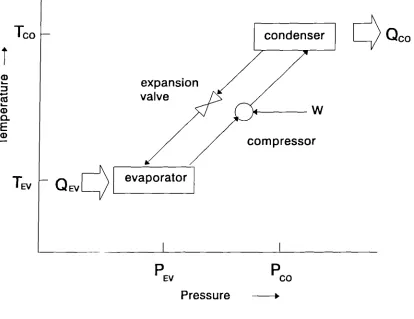
2.2 MECHANICAL VAPOUR COMPRESSION SYSTEMS

The most common type of cooling system is the vapour compression system using a mechanical compressor as shown schematically in Figure 2.1. It consists of two heat exchangers, a compressor, an expansion valve and a working fluid. In the evaporator heat exchanger, the working fluid evaporates at an absolute temperature To, extracting an amount of heat Q Ey from the source which may be in the gaseous, liquid or solid state.

The working fluid is then compressed and gives up an amount of latent heat Qco at a higher absolute temperature Too in the condenser heat exchanger. The condensed working fluid is then expanded through the expansion valve and is returned to the evaporator to complete the cycle.

From the first law of thermodynamics, the amount of heat delivered Qco at higher

temperature Teo is related to the amount of heat extracted Q, at lower temperature TEv

and the amount of high grade energy input W by equation (2.1)

and

COP

H

QCO _

-C°PACL

-W

QEV

W

QC()

QCO-QEV

QEV

QCO-QEV

(2.2)

(2.3)

COPca. — (2.5)

6

The coefficient of performance (COP) of a compressor driven vapour compression

cooling system can be written in the forms

where COP. is the coefficient of performance for heating and COP- ACL is the coefficient

of performance for cooling.

From equations (2.1-2.3) the coefficient of performance for heating is related to the coefficient of performance for cooling by the equation (2.4)

COP

H

= C0PcL

For the theoretically ideal case of zero increase in entropy, the Carnot coefficient of performance of the mechanical vapour compression system shown schematically in Fig. 2.1 can be written

TEV

7

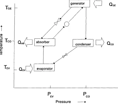
2.3 HEAT DRIVEN ABSORPTION SYSTEMS

The absorption system is different from the compression system. It uses heat energy instead of mechanical energy to make the change in the conditions necessary to complete a refrigeration cycle. This less common type of refrigeration system is shown in Figs. 2.2 and 2.3. The condensation, expansion and evaporation are the same as in the conventional compressor driven system. However, in the absorption cycle, the compressor is replaced by a secondary circuit in which a liquid absorbent is circulated by a pump. The evaporated refrigerant is absorbed by the recirculating liquid and the pressure is increased by the pump prior to entering the generator. An amount of high grade heat Q0E is added at an

absolute temperature TOE in the generator to produce the high pressure refrigerant vapour

required to feed the condenser. [Best et al (1986)]

The mechanical energy required to pump the liquid is usually negligible compared to the input of high grade heat energy QGE•

The pump in the secondary circuit of an absorption heat pump provides the compression ratio CR =

The coefficientcoefficient of performance of a conventional absorption cooler can be defined as

QEV

C ° PACL - (2.6)

QGE

TEV TCO - TEV

COPccL = (

1

8

QEV+QAB

COPAH - (2.7)

QGE

The Carnot coefficient of performance of the heat driven absorption cooling system is shown schematically in Figs. 2.2 and 2.3, can be written as

2.4 AMMONIA-WATER HEAT DRIVEN ABSORPTION COOLING SYSTEMS.

The ammonia-water absorption system technique is a specific example where the vaporizing refrigerant is ammonia and the absorbent liquid is water, or dilute aqueous solution of ammonia (weak solution). The absorber then produces a concentrated solution of ammonia in water (strong solution). This rich solution is separated by evaporation and distillation into two streams-a liquid ammonia overhead product (recycled as refrigerant) and the water-rich (weak solution) used as absorbent. Figure 2.4 shows the basic flow sheet for the ammonia-water absorption system installed at Cerro Prieto Geothermal field. [Bogart (1981)1.

The main parameters that define the performance of an ammonia-water absorption refrigeration system are as follows. From thermodynamics and from mass and heat balance considerations, with reference to Fig. 2.4, [Best et al (1986)] and using the above defined nomenclature, the actual coefficient of performance is given by equation.

QEV

COP A - (2.9)

-

_(2.12)

NREc —

(2.14)

9 The actual coefficient of performance already defined by equation (2.9) can also be written as

MR

(Hp-Ho)

COP

-

(2.10)

M

where Hg is the enthalpy per mass unit of the vapour-liquid mixture leaving the generator. The Carnot coefficient of performance is given by

(

T

—T

C

P

(2.11)

TOE _(TCO—TEV)

and the theoretical coefficient of performance based on enthalpies is

(Ho -Ho)

li

H

(H

-}1

) FR

where FR is the flow ratio and is defined as the ratio of the mass flow rate of solution from the absorber to generator, to the mass flow rate of refrigerant from the condenser and to the evaporator.

Alternatively the flow ratio can be rewritten in terms of concentrations as:

XR — XoE

FR —

( 2 . 13 )

X

The efficiency of the recuperator is given by

-

_(2.15)

10 where 1-143 is the enthalpy of the ammonia/water solution with concentration X, but at the

temperature T3.

The efficiency of the generator is defined as

H7 - H8

H7 - Hv8

where H„ is the enthalpy of the vapour-liquid mixture leaving the generator at the geothermal vapor temperature T. [Best et al (1990)]

2.5 REFERENCES

2.1 R. Best, C. L. Heard, H. Fernandez and J. Siqueiros, Developments in geothermal energy in Mexico-Part five: The commissioning of an ammonia/water absorption cooler operating on low enthalpy geothermal energy, J. Heat Recovery Systems 6 (3) 209-216 (1986).

2.2 R. Best, C. L. Heard, P. Pella, H. Fernandez and F. A. Holland, Developments in geothermal energy in Mexico-Part twenty six: Experimental assessment of an ammonia/water absorption cooler operating on low enthalpy geothermal energy, J. Heat Recovery Systems & CHP, 10 (1) 61-70 (1990).

2.3 A. D. Althouse, C.H. Turnquist and A. F. Bracciano, Modern refrigeration and air conditioning, The Goodheart-Willcox, CO. Publ. South Holland 11, pp 73-99, (1982).

2.4 M. Bogart, Ammonia absorption refrigeration in industrial process, Gulf Publ. Co. Houston, Tx, USA. pp 30-31, (1981).

condenser

expansion

valve

W

compressor

11

1----

evaporator

PEV PCO

Pressure

12

PEV

Pressure

P c 0

generator

QGE TGE

-I

QAB(1 absorber _condenser

A

Q

TEV _evaporator

1 1

13

condenser generator

10

9

pump

low pressure wvalve

V 2

expansion

5 ecuperator

#

evaporator absorber

QGE TGE

high pressure

QAB TAB

14

co

0

Co

Hr CO

0 0

co

0

0

C.)

14

p. 0 14 A0

No

•

0

I co

.0 ₀ .5 2 15 •

0 it

\ I

Co

Co

15

CHAPTER 3

THERMODYNAMIC CONSIDERATIONS FOR

FLUIDISED BED HEAT EXCHANGERS.

3.1 VERTICAL FLUIDISED BED HEAT EXCHANGERS

The principle of operation of a typical vertical fluidised bed heat exchanger is shown in Fig. 3.1. [D. G. Claren, (1989)]. Externally the fluidised heat exchanger resembles a conventional vertical shell and tube heat exchanger. However, internally within the tubes small solid particles are kept in a quasistationary fluidised condition by the liquid passing up the through the tubes. In this context, "quasistationary" means that the continuous swarm of particles is carried by the liquid in the tubes from the inlet channel to the lower section of the outlet channel. In the outlet channel the particles disengage from the liquid and are returned to the inlet channel through a number of downcomer tubes.

Practical application of this principle requires that the particles be evenly distributed over all the tubes. In this way the stability of the multiple parallel fluidised beds is guaranteed. The particles must not leave the outlet channel of the heat exchanger. This can be summarized as follows.

(i) The solid particles have a slightly abrasive (or polishing) effect on the wall of the heat exchanger tubes, so that any deposit will be removed at an early stage.

16 In this work a vertical liquid fluidised bed heat exchanger was studied using sand particles as the bed material and the experimental equipment is a single concentric tube heat exchanger. See Fig 3.2, [C. Heard, (1989)]

3.2 PROPERTIES OF FLUIDISED BEDS

The fluidisation literature deals mostly with gas/solid systems for it is in these that most applications have arisen. The very few fundamental studies of liquid fluidised beds have involved particles of carefully characterized, uniform shapes and smooth surfaces.

In the present application silica sand was used because of its availability, low cost and surface affinity for silica deposition. However sand particles are neither smooth nor uniform and they do not behave in strict accordance with the correlations that describe more idealized fluidised systems.

Fluidisation Velocity

A major constraint on sizing a fluidised bed is u, the minimum superficial velocity (i.e. the fluid velocity relative to the particles) for fluidisation. The vertical pressure drop in the bed is given by; [R. Axtmann, 1986]

inPb = ( 6 8 — 6 f) ( 1 — E md linif( g / ge) (3.1)

where 8, and of are the densities of the solid particles and the fluid, Emf is the voidage

(approximately 0.4 for most granular material at rest), IL is the height of the bed at umf,

Ung — (3.2)

umr — (3.3)

17 remains constant, as does inPb .

According to the Carman-Koseny equation for fine particle fluidisation,

' mf'—'' b

5(1 — en.,f ) 2 S 2 oillimf

where S. is the surface area per unit volume of a single particle and A the viscosity of the fluid. Since (1-E)H is constant, combining eqs 3.1 and 3.2 gives

e3mf ( 6 8 . 6f) g

5(1 — emf)S2d.hge

For uniform spherical particles, S. = 6/dp where dp is the particle diameter; then, for E = 0.4

d(6,-6f)g

umf = 0.00059 (3.4)

WI

Void age

Fluidised beds are universally characterized by an empirical equation that relates the voidage, E, to u, the superficial velocity of the fluid, [J. Richardson, (1954)]

U

e n =

18 where the ut is the terminal (free-falling) velocity of a single particle in the fluid. Equation 3.4 has no theoretical basis and the exponent

n

3.3 REFERENCES

3.1 D. G. Claren and R.E. Bailie, The non-fouling fluidised bed heat exchanger, Heat transfer equipment fundamentals, Design, applications, and Operating problems. The American Society of Mechanical Engineers, Book No. H00500, pp 276-278, (1989).

3.2 C. Heard, preliminary design (1989)

3.3 R. C. Axtmann and D. Grant-taylor, Desalination of geothermal wastewaters in fluidised beds, Geothermics, 15, No. 2, 185-191, (1986).

Fig 3.1 Vertical fluidised bed heat exchanger

19

outlet

inlet

20

fluidised bed

21

CHAPTER 4

EXPERIMENTAL STUDIES WITH AN

ABSORPTION SYSTEM FOR COLD STORAGE

4.1 INTRODUCTION

Mexico possesses large amounts of geothermal energy at temperatures which are too low to enable electricity to be generated efficiently and economically. Of the possible non-electric uses of low and medium enthalpy geothermal energy, the one which appears to have the greatest potential is to use the heat driven absorption systems to provide cold storage facilities for perishable food. It has been estimated that perishable food losses in Mexico, resulting from inadequate handling and cooling facilities, vary from 35 to 50% with sea food having the highest losses [ R. Best, 1990]. Spauschus [Spauschus, (1987)] has published data on the world market for refrigeration and air conditioning equipment. The study showed that North America, Japan and Europe produce and purchase almost 90% of the refrigeration equipment in the world, although they account for less than 25% of the world population. The Middle East, Africa, China and the USSR, with 59% of the world population, produce and purchase less than 5% of the refrigeration equipment in the world. Latin America, with 10% of the world population, produces and purchases 6% of the refrigeration equipment in the world.

22 Most of the geothermal fields in Mexico are located near important agricultural areas. The largest geothermal field in Mexico is at Cerro Prieto which is near the growing city of Mexicali in Baja California. Mexicali is on the border with the U.S. state of California.

In order to continue proving the technical feasibility of operating heat driven absorption cooling systems on low enthalpy geothermal energy, the prototype installed in the Cerro Prieto geothermal field was evaluated under other operating conditions.

This prototype ammonia-water absorption refrigerator used in previous experiments, was originally designed for, and installed in the Los Azufres geothermal field, [Best et al (1986)], and was operated successfully at the Cerro Prieto geothermal field using low enthalpy geothermal steam, under extreme hot weather conditions and high cooling water temperatures [Best et al (1990)].

In order to evaluate the ammonia-water absorption system installed at the Cerro Prieto geothermal field in long test periods, two 24-hour tests were performed to observe its efficiency with ambient temperature variations, and to find out how many changes to the system are required in order to maintain generation and evaporation temperatures. The previous testing periods ranged between 6 to 7 hours for each test.

Another series of tests was performed with the same system in order to complete the data base with generation temperatures between 125 and 90°C and 9.46 x 10-5m3 s (1.5 gpm) of weak solution.

23 (i). to find the system parameters that are going to be corrected, in order to maintain the steady state conditions during ambient temperature variations,

(ii) to estimate the total energy consumption of the system in order to evaluate its economic feasibility,

(iii) to calculate the main parameters of the system in order to define its performance,

and

(iv) to observe how the modifications to the original unit can help obtain a

better performance from the system

4.2 EQUIPMENT

Figure 4.1 is a schematic diagram of the experimental absorption cooler which was installed at the Cerro Prieto Geothermal field. The unit was designed for fabrication at minimum expense. The helicoidal coil in the generator and in the rectifier were the only components made of stainless steel. This was necessary to minimize corrosion and scaling during its contact with geothermal fluid. The other components were determined by the availability of materials.

24 the air entering the evaporator and the saturation temperature of the working fluid in the evaporator.

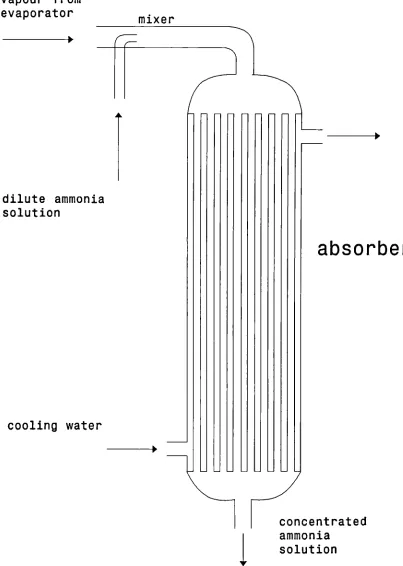
The absorber is illustrated in Fig. 4.2. It consists of a vertical one pass shell and tube heat exchanger. The internal diameter of the shell was 0.20 m and the tube bundle contained thirty six tubes with an internal diameter of 0.2 m. Dilute ammonia solution was mixed with ammonia vapor before entering the absorber in order to enhance heat and mass transfer. The absorber was 1.8 m long.

The generator was a shell and tube heat exchanger. The generator is illustrated schematically in Fig. 4.3. The 1 m long shell was made of available tube with an internal diameter of 0.318 m. Geothermal steam entered at the bottom of the shell and was distributed through a perforate vertical pipe with internal diameter of 0.027 m in the centre of the surrounding coil. The ammonia-water solution circulated through the 17.3 m long stainless steel helicoidal coil which had an internal diameter of 0.0158 m.

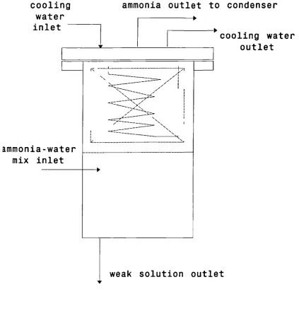
The rectifier was a separator/rectifier unit. This consists of a single vessel with

a

The solution pump used was a piston pump unit. The evaporator was located inside

a

25 The storage chamber was constructed with 0.05 m thick polyethylene and covered by a 0.06 m thick wood sheet.

Additionally there are two more detailed diagrams of the complete system Figs. 4.5 and

4 .6.

4.3 EXPERIMENTAL PROCEDURE

The system was operated manually. Initially the system was charged with 49.3 kg of water and 37.5 of ammonia and 0.74 kg of sodium dichromate as a corrosion inhibitor. Geothermal steam was fed to the generator and the pressure and temperature were controlled until the required steam temperature was reached. When the pressure of the ammonia solution in the generator increased to the operating value, the solution pump and the evaporator fans were turned on. The system was controlled by fixing the solution and the refrigerant flow rates . This was accomplished by manipulating the liquid refrigerant expansion valve between the precooler and the evaporator and the ammonia-water solution expansion valve between the recuperator and the mixer.

The various temperatures, pressures and flows were continuously recorded during each run. For a particular geothermal steam temperature, steady state conditions were achieved when the flow readings in the rotameters and the liquid levels in the accumulators were constant.

4.4 RESULTS AND DISCUSSIONS

26 Table 4.1 shows the main thermodynamics parameters for each test, during 1990.

Tables A1-1 to A1-10 in Appendix 1 show all the data recorded during the experimentation; at the bottom of each column an average and standard deviation of every parameter are shown in order to see the stability of tests.

Figure 4.7 shows the relationship between the actual flow ratio FR, compared with the thermodynamic flow ratio FR. The last test of September 10th and 11th, revealed some problems with the flow relations. The low generation temperature produced low refrigerant flows and since the flow meter scale begins at 6.31 x 10- 6 in' s-1 (0.1 gpm) it is hard to read the exact data, when the flow is lower than that.

Figure 4.8 is a plot of actual coefficient of performance COP, against actual flow ratio FR,. This confirms the observation made by Best [Best et al (1990)1 that at lower values of the flow ratio the system operates at higher efficiencies.

Figure 4.9 is a plot of efficiency of the generator against flow ratio. It can be seen that the efficiency of heat transfer from the geothermal steam to the ammonia/water solution in the generator varied from 0.67 to 0.94. Evidently, the efficiency of the generator is also greater at lower flow rates due to heat losses and steam flow control problems at lower steam flow rates.

27 Figure 4.11 is a plot of the efficiency of the recuperator NREc against values of actual flow ratio.

Figure 4.12 is a plot of the enthalpy coefficient of performance COP E„ and actual coefficient of performance COP, against generator temperatures. It can be seen that the coefficient increases with increasing generator temperatures.

Figure 4.13 and 4.14 are plots of ambient temperature, cooling water temperature and cold storage temperature against time in the two 24-hours tests. They show the stability of the system.

4.5 CONCLUSIONS

It can be shown that the ammonia-water absorption refrigerant system can have a good performance for long periods, with a minimum of control.

The experimental data obtained will be added to the data base and will be used to improve the design and operation of the system and will provide an excellent basis for the design of large scale heat driven absorption refrigeration systems.

4.6 REFERENCES

4.1 R. Best, C. L. Heard, H. Fernandez and J. Siqueiros, Developments in geothermal energy in Mexico-Part five: The commissioning of an ammonia/water absorption cooler operating on low enthalpy geothermal energy, J. Heat Recovery Systems & CHP, 6 (3) 209-216 (1986).

28 ammonia/water absorption cooler operating on low enthalpy geothermal energy, J. Heat Recovery Systems & CHP, 10 (1) 61-70 (1990).

4.3 H.O. Spauschus, Development in refrigeration: technical advances and opportunities for the 1990, Int, J, Refrig. 10 (5), 263-270 (1987).

4.4 International institute of refrigeration, Thermodynamic and physical properties of ammonia, Paris, France (1980)

4.5 Institute of Gas Technology, Physical and thermodynamic properties of ammonia-water mixtures, Research bulletin no.34 (1964).

4.6 CRANE, Flow of fluids through valves, fittings, and pipe, Crane Co. (1978). 4.7 Bogart M., Ammonia absorption refrigeration in industrial processes, Gulf

29

Table 4.1

Main thermodynamic parameters of the absorption system as cold storage tests.

Date: Aug 17 Aug 21 Aug 29 Aug 30 Aug 31 Sep 6 Sep 7 Sep 10 Sep 11 Sep 11*

COPA 0.348 0.421 0.413 0.340 0.280 0.345 0.367 0.333 0.327

*

NREc 0.655 0.695 0.927 0.647 0.576 0.640 0.648 0.654 0.604 *

NGEN 0.836 0.937 0.924 0.787 0.810 0.781 0.757 0.726 0.669 *

FR A 6.839 5.031 7.065 8.955 10.000 8.411 8.654 10.510 12.000 *

T G 113.8 116.2 121 118 125 114 111 107 101

*

1..

0 0

hi

C.1

tms

2 0 0 0 0

0

0 lc

I. ic 0

A

•

g 0 .0_•

•

ea

0

30

8

0 0.

r

absorber

^

-n

_ _ _ _ _ _

1

I

concentrated

i

ammonia

solution

-A

31

vapour from

evaporator

mixer

dilute ammonia

solution

cooling water

32

vapour/liquid mixture

generator

concentrated ammonia

solution

4

condensate steam

cooling

water

inlet

ammonia outlet to condenser

33

ammonia-water

mix inlet

cooling water

outlet

weak solution outlet

O •

L 4-, 0 O 4-, L

o L

0. oo O CD c

> 0 0

• co

•c].

0- 0—zs –,v

0

JatoopaJd

41JelaiumOTS1

CO 4-,

4-, CO

1

ZEIA

JalammoTj.

WC)

34

L

b-fx,

r_

a)

Ca

co

4-, 1

C-CU—

co

I

I-

-1

35

•-I

36

7 r\J

0

L11 Cs] .-1 6

)1‹

37

)1( ₎₁₍

)1(

03 s.0 cs]

)1(

38

39

CO

•:1"

Ct,

•13

)1( )1(

)1(

40

CO

0

0

aJ

CO ch.

Cr)

0

00

0

0

4-3

to

4-5

41

CD

(a0) eati p mio;lad lo quaToTjjaoD

I

-NE

1

o

in o7r om oal 0 0 0

1

0

0

3preJri-12Jedwei

42

L W 4-( ES 0) c O 0

o 0

U o

o

X

ED ED CV , a) E H

1 I _x I

w w w w )1( x w 0 CD E 0 w )1( -)1( x * * 0 0 0 0 0 X L G) 4-) (0 I 1 ED o

ED ED ED 0 o

CV 0 1 I ED Ln ED ED CV

C3=0

-44

CHAPTER 5

EXPERIMENTAL STUDIES WITH AN ABSORPTION SYSTEM USED AS

AN ICE MAKING MACHINE.

5.1 INTRODUCTION

Another potential application of the heat driven absorption cooling systems using the waste geothermal heat is to produce ice for perishable food during transportation and for other cooling uses.

The ice can be produced in these systems using the evaporator as the ice-generator in order to freeze water. The ice could be produced in blocks, cylinders, plates and more forms.

In this experimental study three ice-generator prototypes were constructed and connected to the experimental absorption cooling system and then were evaluated in order to find one that worked in the Cerro Prieto conditions. The three ice-generator prototypes studied were as follows;

1) Vertical Tubes

2) Inclined Plate with Tubing Coil 3) Vertical Tube Coil

45

5.2 VERTICAL TUBES ICE-GENERATOR

5.2.1 Introduction

In order to evaluate the ammonia-water absorption system as an ice-making machine, a vertical tubes ice-generator (VTIG), was designed and constructed [Pefia P. (1988)1. This VTIG was incorporated in the experimental absorption unit. The VTIG was designed to substitute the evaporator diffuser and to produce ice in a batch process. The VTIG design takes into account an ice generator as a heat exchanger in the low pressure zone of ammonia/water absorption cooler.

Two stages in the batch process were considered. One is the freezing time and the other one is the melting time, this latter considers a certain defrost time to separate ice from the generator surface and some additional time for the necessary auxiliary operations to obtain the ice.

Thermodynamic considerations

The main considerations in the ice-making machine design were that [Best and al 19781: QEV = 6 kW

COP, = 0.3 The design conditions were:

refrigerant, ammonia R717 Tf = 0 °C

Tx = -10 °C _{Tjf = -5 °C}

Px = 290.83 _{cy, = 4.18}

Tv,1 = 30 °C _{cif = 2.094} Tk = 35 °C

ri =335 = 1351.0

46

c

T

T

c

1

qj = 471.08

Considering that the percent of freezing capacity is about 80 %, of the theoretical, the amount of ice obtained with the given evaporator capacity could be calculated as follows:

0 .

8

—

24 • 3600

(5.2)

cli

14,

= 880.36 kg day4

This consideration did not take account of losses in defrosting, which could be accepted

as between 0.5 to 2 mm of defrosted ice thickness, between the ice and the generator surface.

Coefficient of performance

The main parameters that define the performance of an absorption refrigeration system are as follows.

From a thermodynamic analysis and from mass and heat balance considerations, using the above defined nomenclature for the process, illustrated in Fig. 5.3, the actual coefficient of performance is given by equation (5.3).

QEV

COPA

_(5.3)

QGE

The actual coefficient of performance already defined by equation (5.3) can also be rewritten as

M

COPA -

(5.4)

47

where H. is the enthalpy of the vapour-liquid mixture leaving the generator.

The coefficient of performance in the ice generator can be written as

Q10

COPm — (5.5)

QEV

The ice-generator actual coefficient of performance already defined by equation (5.5) can also be rewritten as

Mw (1-11—Hw)

COPm — (5.6)

MR (1117—H15)

where Mw is the mass flow of ice generated in kg.s-i.

5.2.2 Equipment

The physical model proposed is an evaporator with vertical tubes, where the generation surface is the tube exterior surface in contact with the water, see Fig 5.1.

The final design was performed with nominal 2 inches tubes and the final installation had to be modified in the field according with the space availability during the installation.

48 flows up inside the vertical tubes' righthand side compartment, then flows down inside the vertical tubes' lefthand side compartment to the lefthand compartment in the refrigerant header, and finally return to the absorber. The water in the recipient is cooled and the ice will be formed in the external surface of the vertical tubes.

The main modifications to the original flow diagram are that the refrigerant coming from the precooler is expanded in an accumulator, then is pumped to the ice generator and returned to the accumulator as a liquid/vapour mixture. At this point the liquid refrigerant goes down and the vapour goes to the precooler and absorber. See Fig. 5.2 and 5.3

5.2.3 Procedure

The refrigeration system was operated in the customary way. The refrigerant expansion point was located at the recirculation receiver tank and liquid refrigerant was accumulated. After the refrigerant level in the tank reached the level indicator, the recirculation pump was turned on. See Fig. 5.3.

At this point the pump outlet pressure did not increase. It is possible that the pump had cavitation problems due to refrigerant evaporation. During 2 hours the refrigeration system produced liquid refrigerant and it was accumulated in the recirculation tank and ammonia was fed to the unit. However the recirculation pump pressure never increased.

5.2.4 Results and Discussions

49 Since the ice generator did not work as it was originally designed and installed, two modifications to the process had to be carried out.

(a) In order to feed refrigerant directly to the ice-generator, a bypass line to the recirculation receiver tank was installed and two additional preliminary tests were performed. During these tests, the refrigerant did not enter the ice-generator because it was bypassed through the solenoid valves due to leaks in them and it returned to the absorber. See Fig. 5.4. This could be detected due to lower temperatures in the returning refrigerant line and some solenoid valves.

(b) In order to approach the refrigerant expansion point to the vertical tubes ice-generator and to correct the leaks in some solenoid valves, a new arrangement with manual valves was installed on the refrigerant lines in the ice generator. See Fig. 5.5.

50 During these tests the vertical tubes were cooled only about 10 cm above the refrigerant header. This could only happen due to an imperfect seal between the vertical tubes' compartments. See Fig. 5.6.

It was possible to observe that the internal plates in the ice-generator vertical tubes were loose, due to noises when the ice-generator tubes were manually beaten.

5.3 INCLINED PLATE WITH TUBING COIL ICE-GENERATOR

5.3.1 Introduction

In order to minimize the amount of water to be cooled the vertical tubes ice-generator is to be substituted by a inclined steel plate ice-generator, (IPIG), in which the water is sprayed over the inclined wall to produce the ice, the excess water is recirculated. See Fig. 5.7.

Two stages of a discontinuous process were considered. One is the freezing time and the other one is the fusion and recuperation time.

Thermodynamic considerations

The main considerations in the ice-making machine design were that [Best and al 1978], [Pella P. (1988)]:

QE , = 6 kW COPA = 0.3

51

refrigerant, ammonia R717 = -10 °C

P. =

w

T

k

Where;

Tf = 0 °C

T

if

w

= 2.094

ri =

q

i

1

f

w

1

qj = 500.13

Also, considering that the percent of freezing capacity is about 80 %, the amount of ice obtained with the given evaporator capacity could be calculated as follows:

0.8

Ma 3600

q,

M, = 34.56 kg h4

Considering that the plate has a surface of 1.77 m 2 , it is possible to obtain ice with 1.92 cm of thickness every hour, this consideration did not take into account losses caused by defrosting. Between 0.5 to 2 mm of defrosted ice thickness between the ice and the generator surface would be acceptable.

52 with 37.5 TON of refrigeration, (Standard Rating Conditions: 15 °C entering water, -18

°C liquid and 2.05 bar at evaporator). It is possible to obtain 15.16 kg IV of ice, with the actual capacity of 6 kW.

5.3.2 Equipment

The old ice-generator recipient, without the bottom part was used in the construction of the new ice-generator. A new inclined bottom was installed with 3 0 of inclination to collect the water on one side. Then the inclined plate was constructed using steel of 0.0016m thickness, and the coil was built with 24m of stainless steel tubing with an internal diameter of 12.7mm. The recirculation water tank has a capacity of 30 litres and the recirculation pump is the same as previously used. See Fig. 5.7. and Fig. 5.9.

The plate has one refrigerant header at the inlet and another at the outlet. This permits the introduction of refrigerant at three points on the inclined plate. The separation between the tubes lines in the coil was about 6 cm due to the tube bends being manufactured with a tool that only allows 6 cm diameter bends. See Fig. 5.8.

5.3.3 Procedure

53

5.3.4 Results and Discussions

In order to prove the IPIG, three preliminary tests were carried out on the whole system. The refrigeration system was operated in the customary way. The refrigerant expansion point was located in the bottom part of the inclined plate (back side) and the outlet was connected to the absorber in the upper part. See Fig. 5.8. Liquid ammonia entered the tubing coil on the bottom part. It flowed upwards inside the coil and returned to the absorber through the upper part. The water flowed down over the inclined plate (front side), but the water temperature did not decrease.

During these tests the whole tubing coil quickly cooled due to the insulation on the back part of the inclined plate and to the poor heat transfer from the tubing coil to the inclined plate.

It was observed that the surface of the inclined plate was cooled only 1 cm above and below each tubing line, in such a way that approximately 4 cm, (the rest of the surface) were not cooled. Additionally, some lines of the tubing coil were separated from the inclined plate by about 1 to 2 mm due to an irregular plate surface, resulting in such parts of the plate not being cooled. It was also observed that the plate was cooled over a very small part of its surface and after one hour of operation, with a coil temperature (expansion temperature) of about - 7°C the water temperature increased from 28 to 33°C.

54

5.4 VERTICAL TUBE COIL ICE-GENERATOR

5.4.1 Introduction

In order to increase contact surface between the liquid refrigerant and the water, a new vertical tube coil ice-generator, with horizontal spaced lines, (VTCIG), was designed.

This tube coil was designed to utilize all the external surface of the 1.22 cm (0.5 inches) of nominal steel tube diameter. This was connected by bends and separated by 2.5 cm (1 inch) with steel plate. See Fig. 5.10.

Two stages of a discontinuous process were considered, one is the freezing time stage and the other one is the fusion and recuperation time stage.

Thermodynamic considerations

Considering that the absorption system has a capacity of 6 kW of cooling and according to the thermodynamic considerations included in Section 5.3.1., 15.16 kg of ice could be produced.

5.4.2 Equipment

55 The vertical tube coil was painted, with epoxy paint, and installed in the system. The vertical tube coil has the refrigerant inlet in the bottom part and the outlet in the top part. The refrigerant flows up inside the tubes. The water was sprayed over the top part through two tubes provided with small holes using

a

5.4.3 Procedure

Figures 5.11 and 5.12 show the VTCIG flow diagram. The freezing surface is the external area of the tubes. The water is pumped from the recirculation water tank and sprayed over the top of the tube coil. Some water is frozen and the remainder flows down to the recirculation water tank. With this process, the amount of water to be cooled was 30 litres. Hot water is not fed until the next cycle. When the ice is formed, the hot vapour from the rectifier are used to separate the ice from the surface. Finally, the ice is collected in the bottom part of the ice-generator.

Next there is a experimental procedure description: Step Description

(a) The absorption system is started up in the customary way.

(b) When liquid ammonia is produced in the condenser, the valve at the inlet of the mixer is opened. This permits the ammonia to flow through the ice generator. The refrigerant valve at the evaporator inlet is normally open. The hot ammonia vapour valve is normally closed.

56 (d) The parameters of the ice-generator are recorded every 5 minutes.

(e) When the ice is formed in the ice-generator, the recirculation water pump is turned off (15 to 25 minutes)', the refrigerant valve after the flowmeter is closed, and the hot ammonia vapour from the rectifier valve is opened. This permits the hot ammonia vapour to flow through the ice-generator coil and release the ice. The strainer in the recirculation water line is cleaned.

(f) When the ice is released from the tube coil walls, the hot ammonia vapour valve is closed and the refrigerant valve is opened. The hot ammonia vapour flows for 1 to 2 minutes. The pressure in the evaporator increases to the pressure in the high pressure side of the absorption system and the evaporator inlet temperature increases to 110 °C. This value decreases when the hot ammonia vapour flow is suspended.

(g) The ice is recovered and weighed. The time used in defrosting and recuperation is 5 minutes.

(h) In order to start another cycle the procedure continues with step (c). (i) If the test is finished, the system is shut down in the customary way.

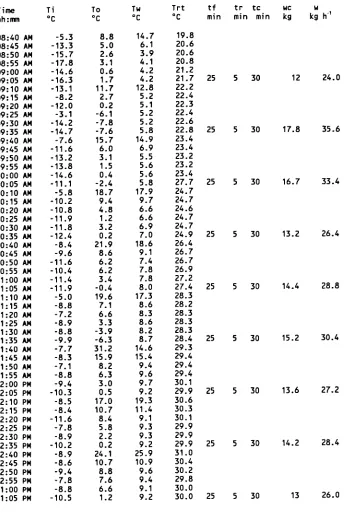
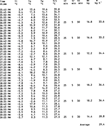
' During the last 2 experimental tests the cycle duration was increased to 30 minutes. With this time 2 periods per hour were obtained and 10 minutes of each hour are used for defrosting and recuperation. This was instead of 20 minute cycles, which have 15 minutes per hour of non-ice production.

5.4.4 Results and Discussions

57 production was only 4 kg 1.14 . An additional water header was constructed using stainless steel tubing of 1.27 cm diameter and the same length. However the number of holes was increased to 86 per tubing spaced every 1.27 cm along the length. Using the tubing water header the water distribution was improved and the ice production was increased to 16.4 kgh-'.

The system was operated at generation temperatures of 130 to 137 °C. These tests were performed at the maximum generation temperatures in order to obtain the biggest ice-production. Also, the temperatures of the brine in the area that could be used for the industrial ice-plant are over 152 °C.

The expansion temperature was -10 °C. The concentration of the strong solution was 43% by weight. See Appendix 1 and Tables A1.11 to A1.16, for the raw experimental data, and the results of the programme REFRI, (Apendix 2), for the thermodynamic evaluation of the ammonia-water absorption system.

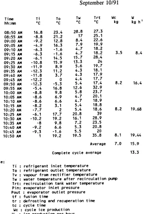
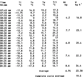
Tables 5.3 to 5.9, show the results of seven tests using the vertical tube coil as an ice-generator. It can be observed that the ice production increases at lower ambient temperatures.

58

5.5 ECONOMIC EVALUATION

Based on the intent of the company Hielo Estrella, S.A. to build a 400,000 kg day l plant to produce ice using the geothermal brine from the Cerro Prieto Geothermal Field, an economic evaluation was prepared based on two kinds of equipment: an absorption system and a mechanical vapour compression.

Table 5.1, shows main data for the analyzed equipment [TURBO, 1988]

The main consideration for the economic evaluation are: (costs are in U.S. Dollars).

• 6,000 hours (250 days) of operating per annum.

• Geothermal brine costs of $0.0581 per TON (180 Mexican pesos) [A. Bacre, 1991]

• Electricity cost of $0.0362 per kWh and $7.23 per kW of maximum demand. • Cost of the two plants at the present time are about 600,000 to 1000,000 however

it can be assumed that the absorption plant cost is 2 times the mechanical compression system cost. [C. Heard, 1991].

• The labour and maintenance costs for the two systems are the same.

The payback period (PBP) for the absorption plant in comparison with the mechanical vapour compression plant would be the additional cost divided by the annual cost of the electricity saved.

Electricity costs absorption plant;

59 Geothermal energy cost, using geothermal brine at 13 bar.

6000*0.0581*202 = 70,417.2 $ per annum Total = 81,498 $ per annum

Electricity costs compression plant

6000*0.0362*6*192 = 250,214 $ per annum.

The amount saved in the electricity is 172,714 US dollar per annum. Table 2 Shows the PBP for a series of electricity costs and plants costs.

5.6 CONCLUSIONS

It was observed that driving liquid refrigerant into the accumulator tank in the vertical tubes ice-generator involves many heat losses.

It was proved that the absorption system has a high coefficient of performance in the vertical tube ice-generator.

It is necessary to test a commercial ice-generator in order to test the absorption system. The actual prototype has many limitations in the amount of labour necessary to produce the ice.

60 5.7 REFERENCES

5.1 P. Pena, Refrigeraci6n por absorci6n amonfaco agua para la producci6n de hielo,

Reporte sobre adiestramiento tëcnico, Instituto de Investigaciones Eldctricas, (1988).

5.2 R. Best, C. L. Heard, H. Fernandez and J. Siqueiros, Developments in geothermal energy in Mexico-Part five: The commissioning of an ammonia/water absorption cooler operating on low enthalpy geothermal energy, J. Heat Recovery Systems 6(3), 209-216 (1986).

5.3 R. Best, C. L. Heard, P. Pena, H. Fernandez and F. A. Holland, Developments in geothermal energy in Mexico-Part twenty six: Experimental assessment of an ammonia/water absorption cooler operating on low enthalpy geothermal energy, J. Heat Recovery Systems 10(1), 61-70 (1990).

5.4 Turbo Refrigerating Company, 1815 Shady Oaks Drive, Denton, Texas 76202, (1988).

5.5 A. Bacre, Personnel communication, Industrias Textiles de B.C. (1991).

5.6 C. L. Heard, Economic and technical justification for the continuation into the

61

Table 5.1

Characteristics of the equipment analyzed for economic analysis

MODEL Nominal Ice Model Compressor Water Feed Units Total

Capacity Number Motor Pump Water required Ice

kg day' kW kW I miff' Production

kg day' Mechanical

compression

72,640 TM-080-0SC 2 0 93.2 3 @ 2 49 6 435,840

Absorption 68,100 TICAR-75-0 3 @ 1 49 6 408,600

Table 5.2 PBP for a series of electricity costs

Electricity Cost USD Total Cost Saved Additional cost for the

per kWh USD per annum absorption plant

PBP years

0.0362 175,714 600,000 3.41

0.0362 175,714 900,000 5.12

0.0362 175,714 1,200,000 6.83

0.1 609,809 600,000 0.98

0.1 609,809 900,000 1.48

0.1 609,809 1,200,000 1.97

0.2 1,290,209 600,000 0.47

0.2 1,290,209 900,000 0.70

62 Table 5.3 Ice-generator experimental data.

September 10/91

Time Ti To Tw Trt Wc W

hh:mm °C °C °C °C kg kg h'

08:50 AM 16.8 23.4 28.8 27.3

08:55 AM -8.8 21.2 17 25.1

09:00 AM -9.2 12.8 8.4 22.6

09:05 AM -4.9 16.3 7.9 19.9

09:10 AM -6.3 -1.6 4.7 18.2

09:15 AM -6.3 -1.6 4.7 18.2 3.5 8.4

09:20 AM -6.1 14.5 15.7 28.4

09:25 AM -10.8 15.9 13.3 24

09:30 AM -11.9 8.9 5.6 19.7

09:35 AM -12.3 11.2 4.3 18.1

09:40 AM -11.8 3.7 4.3 17.9

09:45 AM -12.2 0 4.4 17.7

09:50 AM -12.3 -5.3 5.4 17.4 8.2 16.4

09:55 AM -5.4 16.8 12.6 32.9

10:00 AM -8.8 9.8 5.8 23.7

10:05 AM -8.6 6.9 4.7 20.1

10:10 AM -8.6 6.6 4.7 18.9

10:15 AM -8.2 3.1 5.4 18.8

10:20 AM -7.7 2 5.4 18.6 8.2 19.68

10:25 AM -6.1 17.7 20.8 39

10:30 AM -10.2 19.2 16.1 28.9

10:35 AM -8 9.8 7.2 23.5

10:40 AM -9.2 6.6 5.3 20.8

10:45 AM -9.3 -1.6 5.5 20

10:50 AM 1 19.2 19.5 35.8 8.1 19.44

Average 7.0 15.9

Complete cycle average 13.3

Note:

Ti : refrigerant inlet temperature To : refrigerant outlet temperature Tv : vapour from rectifier temperature Tw : water temperature after recirculation Trt: recirculation tank water temperature Pin: evaporator inlet pressure

Pout : evaporator outlet pressure tf : fusion time

tr : defrosting and recuperation time tc : cycle time

Wc : cycle ice production W : ice production per hour

63 Table 5.4 Ice-generator experimental data.

September 11/91

Time Ti To Tw Trt Wc

hh:mm °C °C °C °C kg kg hl

07:45 AM -11.6 14.9 13.2 17.3 07:50 AM -11.75 9.7 6.2 15.3 07:55 AM -11.3 4.9 2.2 13.6

08:00 AM -11.3 0 2.1 13 4.2 16.8 08:05 AM -5.6 10.6 8.7 18.7

08:10 AM -10.4 8.3 5.6 16.4 08:15 AM -11.2 16.3 19.9 7.9 08:20 AM -11.6 -3.7 3.6 14.4

08:25 AM -12.1 -5.6 4.5 14.2 7.7 23.1 08:30 AM -7.2 14.8 15.1 25.2

08:35 AM -9.1 12.1 9.3 21.2 08:40 AM -12.6 6.7 4.6 17 08:45 AM -14.7 4.8 3.2 15.4

08:50 AM -15.1 3.3 2.8 14.9 6.8 20.4 08:55 AM -16.6 2.7 2.4 14.3

09:00 AM -1.4 11.8 14.2 23.9 09:05 AM -17.8 14.2 11.1 20.3 09:10 AM -18.4 8.2 4.2 17.2

09:15 AM -16.6 3.8 2.2 15.4 7.4 22.2 09:20 AM -17.6 2.2 2.1 14.9

09:25 AM -10.5 12.1 10.6 26.6 09:30 AM -14.3 2.9 2.7 18.3

09:35 AM -17.3 -17.3 8.2 16.1 8.6 34.4

Average 6.94 23.38