The SpinJ model checker : a fast, extensible, object oriented model checker

(1)

Master’s Thesis

in Computer Science

The SpinJ Model Checker

A fast, extensible, object-oriented model checker

Author:

Marc de Jonge

[email protected]

Supervisor: Theo Ruys [email protected]

Committee: dr. ir. Theo Ruys dr. ir. Arend Rensink dr. ir. Marieke Huisman

(2)

Abstract

Model checking has grown to be a practical addition to the field of formal verification. One model checker that has proven itself very useful in practice is

Spin_{, which is built to validate models that are written in} promela_{. It can}

be used to search for deadlocks, assertions, liveness properties and even LTL properties.

This thesis describes the design and implementation of SpinJ_{, a}

reimplementation of Spin _{in Java.} SpinJ _{is designed to be behave similarly}

toSpin_{, but to be more}_extendible _and_{reusable. To achieve this the conceptual}

framework of Kattenbelt is used as the basis for the design of theSpinJ_library,

using the three layers that he describes.

Firstly, the generic layer is the lowest layer which uses a basic model with states and transitions. On this layer all storage methods, search algorithms and simulation techniques are implemented. The abstract layer describes a concurrent model with processes that is an extension of the model in the generic layer. This knowledge of processes within the model makes it possible to implement partial order reduction here. Finally thetool layer is implemented for thepromela_{language support.}

SpinJ _{also contains a} promela _{compiler that generates Java code to}

represent the given promela _{model. This Java code can be compiled and}

then verified using theSpinJ _{library. Since this library contains all the actual}

algorithms, the generated code can be relatively small, only describing the model itself. Also all algorithms that are available can be used with any model and can be selected at runtime.

Despite the fact thatSpinJ _{is designed to be extendible and reusable, it is}

not slow; using the BEEM benchmark, this thesis has shows that SpinJ _{is on}

average only 3.5 times slower thanSpin_{and it uses less memory in most of the}

(3)

List of Figures

2.1 The architecture of Spin _{. . . .} ₆

2.2 Overview of the framework of Mark Kattenbelt . . . 8

3.1 Architecture ofSpinJ _{. . . .} ₉

3.2 Design of theSpinJ _library _{. . . 11}

3.3 Design of theSpinJ promela_compiler _{. . . 13}

4.1 UML diagram of the Generic layer . . . 15

4.2 UML diagram of theObservableModel . . . 19

5.1 UML diagram of the Abstract layer. . . 30

6.1 An example statespace . . . 36

6.2 UML diagram of classes used by thepromela _compiler _{. . . 37}

6.3 Optimising the internal representation . . . 40

6.4 Example of statement merging . . . 41

6.5 Example of removing empty transitions . . . 41

6.6 Example of removing goto-transitions . . . 42

(7)

List of Tables

4.1 Implementation of Depth First Search . . . 23

4.2 Implementation of Breadth First Search . . . 24

7.1 Benchmark comparison without Partial Order Reduction. . . 59

7.2 Benchmark comparison with Partial Order Reduction . . . 60

7.3 Benchmark comparison with Bitstate hashing . . . 60

7.4 Benchmark comparison with Hash compaction . . . 61

B.1 Benchmark result without Partial Order Reduction . . . 77

B.2 Benchmark result with Partial Order Reduction . . . 81

B.3 Benchmark result with Bistate hashing. . . 85

(8)

Preface

First I would like to thank Theo Ruys for his support over the course of this project. Without his constructive comments and discussions during our regular sessions, I would not have been able to complete this assignment. Furthermore I would like to thank Marieke Huisman for her last minute review.

(9)

Chapter 1

Introduction

In any software lifecycle process testing plays an important role [4], taking up many resources. It helps to see if the system meets its requirements, by finding faults in the implementation. A limitation of most testing techniques is that it only covers a few predefined runs, therefore not finding all possible errors. This is especially true for concurrent systems, where different threads can interfere with each other.

To complement standard testing techniques, it is possible to use model checking [29] [7]. This is a formal method that rather than executing a couple of selected runs, tries to verify every possible run in the system. Typically a model checker does not run on the implemented system itself, but on amodel of the system, with specifiedproperties that represent the requirements. Such a formal verification can then be used to verify that the intended model is correct. Three computer scientists - Edmund M. Clarke, E. Allen Emerson, and Joseph Sifakis - pioneered model checking in the 1980s, for which they received the ACM Turing Award [3] of 2007. From [3]: “[They have received the award] for their original and continuing research in a quality assurance process known as Model Checking. Their innovations transformed this approach from a theoretical technique to a highly effective verification technology that enables computer hardware and software engineers to find errors efficiently in complex system designs. This transformation has resulted in increased assurance that the systems perform as intended by the designers.”

One of these model checkers that has proved to be very useful in practice is Spin _[₁_]. _{The creator of} Spin_{, Gerard Holzmann, even received the}

ACM Software System Award, because (from [2]) “(ACM) has recognized Dr. Gerard Holzmann for his contribution to a widely used software package called SPIN that quickly detects defects in networked computers, making them more reliable”.

The models that can be checked by Spin _{are written in the} promela

language, which is specially designed to allow for dynamic creation of concurrent processes. This allows a user to model a distributed system or a protocol. In

promela _{models, communication between different processes can be defined}

(10)

Spin _{can validate models written in} promela _{for deadlocks, assertion}

violations, lifeness properties and even properties expressed in LTL (linear temporal logic, see [17]). It is designed to scale well and to handle even very large problem sizes. To achieve this, it is implemented is plain C, using a monolithic design that is fully optimised for promela_{models. Unfortunately,}

this design makes it more difficult to implement new algorithms or reuse parts of the implementation.

1.1

Problem statement

Is it possible to re-implement the core of Spin _{in Java whilst being competitive}

in terms of memory consumption and runtime behaviour?

This question comes from two underlying questions. First to see if it is possible to create a program like Spin _{that is created using modern,}

object-oriented programming techniques. This would make it easier to reuse parts of the program and to extend it. Secondly to see if Java has the capability to execute such a program in acceptable time and memory usage.

The program that has been created during this thesis is called SpinJ_{. The}

goal is to implement it such that the following conditions hold:

The design and implementation of SpinJ should be object-oriented,

reusable and well documented.

The design and implementation ofSpinJ should beextendable, such that

other algorithms are easily added. It should be possible to extend the modelling language.

The performance of SpinJ should be comparable to Spin (both in time

and space), where one order of magnitude of difference is acceptable.

SpinJ’s simulator and verifier should use the same Java code.

SpinJ should support several of Spin’s optimisation algorithms, e.g.

partial order reduction, bitstate hashing and hash compaction.

The output and parameters ofSpinJshould resemble the ones ofSpinas

much as possible.

1.2

Overview

The rest of this document describes the development of SpinJ_{, a new model}

checker that can verify models written in promela_{. We will start with some}

background information in Chapter 2, where we will discuss some other model checkers like Spin_.

After that, Chapter 3 will give an overview of the architecture of SpinJ_,

(11)

In the chapters 4, 5 and 6 the implementation of the 3 different layers is explained. Each of these layers describes more details of the model, where the lowest layer only knows about states and transitions, the highest layer knows all specificpromela _features.

To see how SpinJ _{performs, a benchmark is used to test it against}Spin _in

(12)

Chapter 2

Related work

This chapter discusses model checking in general and different existing explicit model checkers. Then it describes the design and implementations of Spin

and the conceptual framework of Kattenbelt. This will be kept brief, a more extensive overview is written in [32].

2.1

Model checking

Model checking [35] is the formalverification of amodel against aspecification. To do this it uses a verification algorithm to check whether model (M) models the specification (p), which can be written asM |=p. When an error is found, a model checker shows an error trace on whichp does not hold.

2.1.1 Model Specification

The model is a formal description of a system. This model can be derived from a system, automatically or manually, but can also be created before the system is built. Validating a model before the implementation is used to validate the design or protocol. Models usually abstract from irrelevant aspects of the system, to make the validation easier. Using the system itself as a model is also possible.

A model can be represented in many different forms. Most models are specified in a language and are first transformed to a mathematical model. This mathematical model can then be used by the verification algorithm to prove that all properties of the specification hold.

There are some differences between mathematical models, although they are mostly based on a Labelled Transition System. For example, some types add the notion of clocks (e.g. Timed Automata [5] or Continuous-Time Markov Chains [6]).

A Labelled Transition System (LTS) is one of the most elemental ways to describe a model. It can be defined as a 4-tuple M= (S, s0,Σ, T), whereS is the set of states, s0 ∈S the initial state, Σ is the set of labels (the alphabet) and T ⊆S×Σ×S is the set of transitions.

(13)

state machine adds a set of final (or ending) states F ⊆S to the LTS. Such a state machine accepts a (regular) language with words of finite length.

Another variation is a labelled Büchi automaton, which adds a set of accepting states (A∈S). A Büchi automaton accepts a language with infinite words. For a Büchi automaton to accept such a word, it must pass an infinite number of accepting states. In model checking Büchi automata are used to define “bad” behaviour, as we can define a language that specifies that “bad” behaviour.

2.1.2 Property Specification

There are different ways to define properties that should be checked over an LTS. Three of those are invariants, Linear Temporal Logic (LTL) and Computation Tree Logic (CTL). All these properties are based on the use of atomic propositions.

Atomic propositions These are the most basic elements of any proposition. They simply describe a condition about one part of the model, in a certain state. For example, “x >0” or “processA is blocked” are such atomic propositions.

Invariants The atomic propositions can be combined with logic operators to form formulae. For example, ifpandqare valid propositions,¬p,p∨qandp∧q

are also propositions. The invariants describesafety properties of a single state in the model. This could be defined asassertions on one of the labels (checking the last state) or as global invariants that should hold for every state. These safety properties can be verified by an exhaustive search over all the possible states. When a violation was found, it can then return a finite trace to the error.

Linear Temporal Logic Invariants can be used to specify a property of one state, but it can not be used to define properties over paths in the model. LTL [27] expressions are designed to specify properties over a path in the model (e.g. lifeness properties). For example, it can be used to define that a certain atomic property holds until some other property becomes true.

Computational Temporal Logic As LTL properties are defined over paths, it can not distinguish between paths. CTL [27] can be used in cases where we want to make such a distinction. For example, it is possible with CTL to define that from a certain state there is at least one path where some propertypalways holds.

2.2

Model checkers

We can split model checkers into two different groups:

Explicit state model checkers generate each possible state of the system

(14)

of an exhaustive search over all the states and an on-the-fly validation. Examples of explicit model checkers are Spin_[₁_],nips_[₃₉_{] and} jpf _[₉_].

Symbolic model checkersdo not represent individual states, but they store

sets of states. These sets can be represented symbolically (e.g. in a binary decision diagram). This approach is more effective for checking CTL propositions. One example of a symbolic model checker is SMV [34].

There are other variations (e.g. bounded model checkers like NuSMV [10]), but in this thesis we are going to focus on explicit model checking. The rest of this section is going to discuss a couple of model checkers, showing the design of each and how they are implemented.

2.2.1 Spin

Spin _[₁_{] is arguably the most used model checker, which has proven itself}

on industrial size problems [23]. Gerard Holzmann, the creator of Spin_,

even received an ACM Software System award [2]. Spin _{is still further}

improved. Recently version 5 has been released, which adds support for multicore systems [22].

The model specification language for Spin _{is called} promela_. promela

can be used to model several processes that can be started dynamically. More details about this language will be discussed in Chapter6.

Architecture

X S p i n P r o m e l a

m o d e l

p L T L

t r a n s l a t o r

S i m u l a t o r

V e r i f i e r g e n e r a t o r s p i n . e x e

C p r o g r a m

C o u n t e r

e x a m p l e V e r i f i e r

d e a d l o c k s s a f e t y p r o p e r t i e s l i v e n e s s p r o p e r t i e s

p a n . *

p a n . e x e

S p i n

r a n d o m g u i d e d i n t e r a c t i v e

(15)

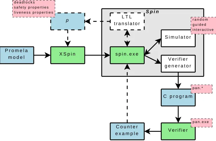
In [19] the basic structure of Spin _{is discussed, which is also shown in}

Figure 2.1. Spin _{itself is the} promela _{parser that can read models that are}

written inpromela_{and do two things with it:}

When the -a option is not set when calling Spin_{, a} _simulation _{is started.}

This simulation can either be guided by the user (interactive), by a generated trace-file (guided) or at random.

When the -a option is set, Spin _{will use the}_{verifier generator} _{to produce}

theverifier. This verifier is highly optimised and written in ANSI C. It can be compiled using any C compiler. When the verifier is run and it finds an error, it can produce a counter-example in the form of a trace-file. This file can be used to guide the simulation.

Implementation

Spin _{is completely written in ANSI C, with speed as its main goal. This has}

a disadvantage in terms of reusability and extensibility. Spin _{is written as a}

“black box”, meaning that the whole application is tightly coupled and it is difficult to identify the different parts.

Also, to keep Spin _{as fast as possible, all of the options regarding to the}

search algorithm, storage techniques etc. are implemented using pre-processor instructions in the generated C-code. For example, if we want a model to use hash compaction [40], we need to compile the generated C-code with the preprocessor option-DHC.

2.2.2 Kattenbelt’s conceptual framework

In his thesis [32], Mark Kattenbelt describes a conceptual framework that unifies the model checking domain. Kattenbelt also created an implementation based on that design that can handle models that are written in Prom+, a simpler variation based on promela _{that adds the notion of dynamic storage and}

pointers.

Architecture

The conceptual framework contains three layers, also shown in Figure 2.2. From [32]:

“The generic layer provides algorithms for certain types of models. [. . . ]

It is not feasible to define just one generic layer for all models, this is due to the diversity of models in the model checking domain. For instance, the fields of explicit-state, symbolic, bounded and probabilistic model checking are too different to be encapsulated within the same generic layer, and should probably be defined in separate generic layers.”

(16)

S t a t e S p a c e

S i m u l a t i o n A l g o r i t h m s

T e s t i n g A l g o r i t h m s

V e r i f i c a t i o n A l g o r i t h m s

S o f t w a r e M o d e l G T S

S P I N P r o m + B o g o r G R O O V E T o o l L a y e r

A b s t r a c t L a y e r

G e n e r i c L a y e r

Figure 2.2: An overview of three layers in the framework that is designed by Mark Kattenbelt.

“The abstract layer is the layer on top of the generic layer. In particular

it gives an internal structure to the generic layer. [. . . ] The idea is that it is possible to have multiple abstract layers on the same generic layer such that the algorithms of generic layers are reused.”

“The tool layer is not provided by the framework, it is included in the

figure to show how tools could use the framework. [. . . ] The nature of the tool layer is that it is not reusable, however, the idea is that a well-defined abstract layer could be used by multiple tools.”

Implementation

Mark Kattenbelt has implemented his framework in C++, and added in the tool layer the support for the Prom+ language. It does not use the complete potential of its design, because of the simplicity of the Prom+ language. Also his benchmarks show that it is much slower thanSpin_{(by a factor 1000) while}

(17)

Chapter 3

Figure 3.1: The architecture of SpinJ

For the design ofSpinJ_{, the main}

ob-jectives of this thesis must be taken into account. First of all, SpinJ

should be extensible and reusable. This means for example that adding a new search algorithm should be easy and such a algorithm should be readily available for all implemen-tations based on SpinJ_{. Secondly,}

SpinJ_{should remain as}_fast _as

possi-ble. A magnitude slower thanSpin_is

acceptable, but it must still be prac-tical for model checking.

The first section of this chapter will explain the overall architecture that was chosen for SpinJ_{. The}

following sections will then explain the design of the two basic parts of

SpinJ_{: the library (Section} _3.2_{), with}

thepromela_{implementation on top}

of it, and the promela _compiler

(Section3.3).

3.1

Architecture

To verify a model that is written in

thepromela_language,SpinJ_follows

Spin_{s compilation architecture.} Spin

(18)

An alternative solution to verify a promela _{model would be using an}

interpreter, although pure interpretation would be slower [38]. Though there are midways between an interpreter and a compiler, in most cases the fastest solution would be the compiler approach.

There is a downside to the architecture ofSpin_{: all code is generated by the}

compiler and no code of the verifier can be reused. This is great for optimising the code, but makes changes more complicated and the algorithms that are provided can not be used directly in other projects.

SpinJ _{tries to take advantage of using generated code like}Spin_{, while still}

making use of a shared library. How this works is shown in Figure3.1. First the compiler generates a Java representation of thepromela_{specification (step 1).}

Then the Java compiler is used to compile the code (step 2) using theSpinJ

promela _{implementation, which in turn uses the general} SpinJ _{library. The}

SpinJ _{library contains much of the shared code, for example search algorithms}

and storage methods. This is the main advantage ofSpinJ_{, because this library}

is designed in such a way that it can be reused. This makes it easier to support other languages: only a basic implementation and a compiler have to be added. After compilation the verifier can be run on any Java Virtual Machine (step 3), to produce the result. On the command line, the following commands would have to be executed to check the model Foo:

1 java−jar SpinJ.jar Foo.prom

2 javac−cp SpinJ.jar spinj/generated/FooModel.java

3 java−cp SpinJ.jar spinj.generated.FooModel

SpinJ.jar contains both the layered library as well as the promela

compiler. On the first line that promela _{compiler from} _SpinJ.jar_{is called,}

which does not use the library at all. The second and third line don’t use the compiler anymore, but do use the library.

3.2

The layered model

For the design and implementation of SpinJ _{we have adopted the conceptual}

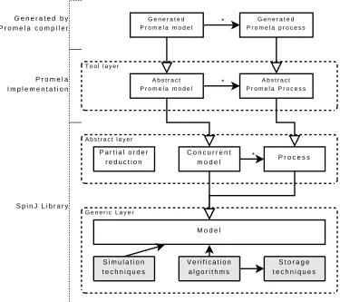
framework developed by Mark Kattenbelt et al. [32]. Mark Kattenbelt showed in his Master Thesis [31] that his framework is more flexible than the “black box” approach of many other model checkers. In Figure3.2our implementation follows this layered model.

The idea behind these three layers is that each layer extends the layer below it and adds more functionality. This is achieved through inheritance (indicated by the open arrow in Figure 3.2). For example, the concurrent model on the Abstract layer extends the model from the Generic layer. This means that all algorithms that can use a model, can also use any concurrent model. On the abstract layer, however, there are algorithms implemented that can use the fact that a concurrent model contains one or more processes.

(19)

A b s t r a c t

Figure 3.2: The design of the SpinJ _{library, with on top the} promela

implementation

3.2.1 Generic layer

The generic layer is the lowest layer, which has a very basic concept of the model. Here we only know that a model consists of states and transitions, not how the model works internally. Despite the fact that we do not know much about the model, we have enough information to implement several important algorithms in this layer. E.g. search algorithms, storage methods and hashing methods.

(20)

3.2.2 Abstract layer

The abstract layer provides us with an extension of the model that was described on the generic layer. It adds the notion of concurrency to the model, where it contains several processes (indicated with the arrow and star in Figure 3.2). These processes can be viewed as models by themselves and the concurrent model generates a Cartesian product of these.

On this level there is also method implemented to optimize the model: Partial Order Reduction. This optimizers can reduce the state space that is generated by the model, by using the fact that the processes are not always depending on each other. For more information see Section 5.2.

The implementation of the abstract layer is described in Chapter5.

3.2.3 The promela _{Tool layer}

Within the tool layer an abstract model is defined that makes it easier to generate Java code from thepromela_{compiler. The abstract}promela_model

is again an extension of the concurrent model from the abstract layer. Also some extra helper objects are implemented here (e.g. the Channel object, for easy simulation of channels).

On top of this layer the generated promela _{models are placed, as an}

extension of the abstract promela _model. _{These generated models are}

the product of the promela _{compiler as described in Section} _6.3_. _The

implementation of the tool layer is described in Section 6.2.

It is possible to adapt SpinJ _{to support different languages by creating a}

new implementation of this layer and of the compiler.

3.3

The

promela

Compiler

The SpinJ promela _{compiler is responsible for translating the} promela

specification to the generated promela _{Java model from Figure} _3.2_{, which}

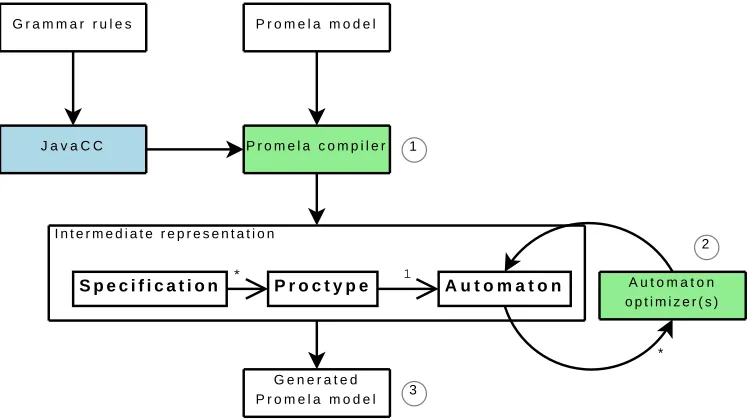
can be used with the SpinJ library to verify the model. In Figure 3.3 we can see this process in three steps.

The first step is translating the originalpromela_{model to an intermediate}

representation. This is done using apromela_{parser. This parser is generated}

using the JavaCC (Java Compiler Compiler) tool. This tool reads a grammar file and converts it to the Java code that makes up the parser.

When this first step is done, we have an intermediate representation where

the Specification object holds all the information. This object contains

one or more Proctype objects (the promela _{processes), which in turn holds}

one Automaton. An Automaton object holds all information concerning the

behaviour of the process, e.g. the possible states and transitions.

The second step optimises theAutomatonobjects to generate a more efficient automaton, which usually contains less states. This is done using one or more

Automatonoptimizers.

Finally the Java code is generated that makes up the final generated

(21)

J a v a C C G r a m m a r r u l e s

P r o m e l a c o m p i l e r P r o m e l a m o d e l

S p e c i f i c a t i o n * P r o c t y p e 1 A u t o m a t o n

G e n e r a t e d P r o m e l a m o d e l

A u t o m a t o n o p t i m i z e r ( s )

* I n t e r m e d i a t e r e p r e s e n t a t i o n

1

2

3

Figure 3.3: The design of the SpinJ promela_compiler

library run as a complete model checker.

(22)

Chapter 4

Generic layer

This chapter will explain how the Generic layer of theSpinJ_{library is designed}

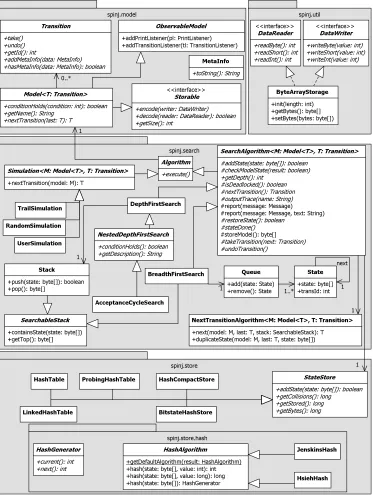
and implemented. Recall that the Generic Layer has a very basic concept of the model (see Figure 3.2). The different parts that will be discussed here are displayed in the UML class diagram of Figure 4.1. As can be seen, this layer contains several methods and algorithms. We can split these into the following categories, with corresponding package names:

The model description (spinj.model). This provides some abstract

classes that have to be implemented by any model, to be verifiable by

SpinJ_{. A}_Model_{object represents here a means to generate a state space}

on-the-fly. On this layer not much more is known than that it consists of states and transitions. This is further explained in Section 4.1.

The simulation methods and search algorithms (spinj.search).

There are several methods available to simulate a given model, which are described in Section 4.2.1. Also a couple of search algorithms are implemented to search trough the state space that can be generated by the model. These are described in Section 4.2.

The storage methods (spinj.store). These are used to store the states

that have been found during the execution of one of the search algorithms. This is needed, because it is more efficient when encountering duplicate states. Now when a state is reached that was stored before, the search algorithm can skip it. The different storage methods are described in Section4.3.

The hashing algorithms (spinj.store.hash). Many of the storage

methods use a hashing algorithm to efficiently store and find states. The implementation of one of these methods is described in Section4.4.

4.1

Model description

(23)

spinj.model

+next(model: M, last: T, stack: SearchableStack): T +duplicateState(model: M, last: T, state: byte[])

1 +hash(state: byte[], value: int): int +hash(state: byte[], value: long): long +hash(state: byte[]): HashGenerator

(24)

To create the states at runtime, a starting state should be known and it should be known how to take a transition from one state to the next. When that transition is taken, the current state of the model is changed. To achieve this functionality, the following function should be implemented by each Model

object:

The nextTransitionmethod: Given the current (implicit) state of the

model and a previous taken transition from that state, it can generate the next transition. This method can be used to compute all the transitions that are enabled in the current state. More details on transitions will be explained in Section 4.1.2.

Theencodemethod: Encodes the current state of the model in an efficient

way. More details will be explained in Section4.1.1.

The decode method: Decodes the encoded data to restore a state that

was stored using the encodemethod.

The conditionHolds method: Checks whether a given condition holds.

The conditions that are provided by default are:

– Whether the current state should be stored, because there are cases when a state should not be stored (e.g. in a atomic sequence in Promela, see Section6.2.5).

– Whether the current state is anend state. This is used when checking for a deadlock. When encountering a state where there are no more transitions that can be taken, we are either in an end state (all activity has ended normally) or in a deadlock situation.

– Whether the current state is in an acceptance state. This is used when searching for acceptance cycles [25]. See Section 4.2.4.

ThegetNamemethod: This method is used to produce a meaningful name

for this model.

The methods from the ObservableModelcan be used to add listeners to

the model. These listeners can listen for two types of events: print events or taking/undoing a transition. This is further explained in Section4.1.3.

4.1.1 Encoding states

(25)

each Java object). Since the state vector of most models is less than 100 bytes, this is a significant overhead.

Furthermore implementing a hash function on a simple array of numbers is easier, than to create an approximate hash function for each generatedModel.

The Storable interface To encode the states, the Model implements the

Storableinterface (see Figure4.1). This interface makes it possible to encode

the current state of the model into a more primitive format (e.g. a byte array). The simplest solution to this would be to have a store function that returns a new byte array that represents the current state, but this solution is not perfect. The problem lies in the performance, because many optimizations are not possible.

Having aencodefunction that can encode the state using theDataWriter, is more flexible. To make this work a getSize method is also available, to indicate how many bytes need to be available to store it.

To see what exactly the advantage of this method is, let us evaluate the next example:

1 public int getSize() {

2 // The model needs to store the number of processes

3 int size = 1;

4 for(Process proc : processes) {

5 // Add the size of each process

6 size+=proc.getSize() ;

7 }

8 return size;

9 }

10

11 public void encode(DataWriter writer) { 12 // First encode the number of processes

13 writer.writeByte(nrProcs) ;

14 for(Process proc : processes) {

15 // Encode each process in the buffer

16 proc.encode(writer) ;

17 }

18 }

This example shows the (simplified) implementation of theencodefunction of a model with a few processes in it as defined in SpinJ_{. To encode all the}

processes, the Process class also implements the Storable interface. Now we can simply call theencodefunction for each process in the model (and the same for thegetSizemethod).

If we had used a storefunction that simply returns a byte array, each call to thestorefunction of each process would have returned a temporary object. This puts more pressure on the garbage collector. The current design handles this more efficiently.

(26)

4.1.2 Transitions

The set of transitions that can be executed from a certain state is called the enabled set. To retrieve the enabled set from the model, the nextTransition

function is defined in the model.

This function does not return the enabled set directly, as one might expect, because of efficiency reasons. To store such a set, a temporary storage object is needed. Furthermore, not all enabled transitions are needed directly when using Depth First Search (which is the default search algorithm inSpin _{and in}

SpinJ_).

Instead, only one transition is returned each time the nextTransition

function is called. To retrieve any further transitions that may be executed, the previous transition is provided as a parameter, until the function returns null, indicating that there are no more transitions. This resembles the iterator and enumeration functionality found in the Java class library.

The Transition class All transitions that are returned from the model,

implement the Transition class. This class describes the following functionality:

Thetakefunction executes the transition, changing the state of the model

to the next state.

Theundofunction undoes all changes that are made by thetakefunction.

This function is called when we want to return to a previous state.

ThegetIdfunction returns a unique identifier that can be used to create

a trail file, which stores the path to a certain state (see Section4.2.6).

As can be seen, each transition has a mandatoryundoaction. Because many transitions change only a very small part of the state vector, it is often more efficient to undo the transition than to decode the complete state vector.

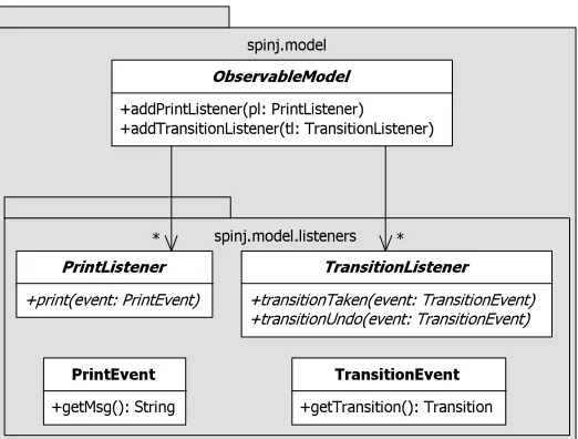
4.1.3 Observable Model

There are two aspects of the model for which the observer pattern [15] is used: changing the state of the model and performing a print action. For both actions a separate interface is defined: the TransitionListenerand the

PrintListener.

To ease the usage of this pattern, eachModelextends theObservableModel

class. This class contains all the functionality to add listeners, notify them and disable or enable them (also described in Figure 4.2).

Now each time a transition is taken in a model, thesendTransactionTakeEvent

(27)

spinj.model

Figure 4.2: An UML diagram that describes the ObservableModel

4.2

Exploration algorithms

A crucial part of a model checker are the exploration algorithm(s) that are supported. InSpinJ _{the goal is to make this part extendable, such that other}

exploration algorithms can be added in the future. In the current version there are several different implementations, which can be split in two categories: search algorithms, which explore the complete state space, and simulation algorithms, which executes a single path through the state space.

4.2.1 Simulation

To see if a given model behaves as expected, the author of that model will usually perform a couple of test runs. This is done in the simulation mode. In simulation mode there is a single path through the state space chosen to be executed.

The Simulation class uses generics to keep track of the type of Model (M)

and Transition(T) it is executing. This type safety is needed for calculating

the next transition, otherwise a (unsafe) cast must be used. Simulation of a model is a simple procedure, as can be seen in the following code example from

theSimulation.executemethod:

1 public void execute() { 2 while (true) {

3 try {

4 // Choose the next transition that we are going to execute

5 final T t= nextTransition(model) ;

6 i f (t==null) { // No next transition , quit

7 break;

8 }

9 out.println(”Taking transition : ” +t.toString() ) ;

(28)

11 states++; // Increase the number of states that were visit ed

12 } catch (final ValidationException ex) {

13 out.println(ex.getMessage() ) ;

14 break;

15 }

16 }

17 }

When a simulation is executed, it chooses one transition to execute for each step. The choice is done in the nextTransition method. Then it takes that transition.

This loop is executed until either thenextTransitionfunction returnsnull

(indicating to end the run), or aValidationExceptionis thrown while taking the next transition (indicating an error in the model).

The current version provides three different implementations ofSimulation:

UserSimulation, which asks the user for choosing the transition to be

taken.

RandomSimulation, which randomly chooses the transition from the

enabled set, until the enabled set is empty.

TrailSimulation, which reads a trail file (see Section 4.2.6) and

chooses the transition with the same identifier (returned by the

Transition.getIdmethod).

4.2.2 Abstract Search algorithm

The implementation of all the search algorithms currently in SpinJ _{are based}

on an abstract search algorithm, which contains some basic code that is the same for every search algorithm.

The difference between different search algorithms is the order in which the states are explored (e.g. a stack or queue of waiting states) and if some states may or may not be explored further (e.g. with dynamic partial order reduction [14] we can optimize the state space). The common denominator between all the possible search algorithms can be described in the following three basic steps:

Retrieving a not yet fully expanded state to expand the search area.

Checking the retrieved state for errors (e.g. deadlocks).

Executing one transition from the current state that has not been executed

yet, resulting in a new state. When this new state was already visited before, it is discarded. Otherwise it is stored and put in the collection of states that need to be expanded further.

(29)

itself (e.g. assertion checks). A simplified version of theexecutemethod in the

SearchAlgorithmclass is given below.

1 public void execute() {

2 byte[ ] state=storeModel() ;

3 addState(state) ; // Adds the i n i t i a l state to the search algorithm

4 i f(model.conditionHolds(SHOULD_STORE_STATE) ) {

5 store.addState(state) ;

6 }

7

8 while(nrErrors<maxErrors&&restoreState() ) {

9 // Make sure that the state matches the internal state of the model

10 assert checkModelState(model)

11

12 // Retrieve the next transition

13 final Transition next=nextTransition() ; 14

15 i f(next==null) {

16 i f (checkForDeadlocks&& !model.conditionHolds(Condition.END_STATE)

17 &&getLastTransition() ==null) {

18 report(DEADLOCK) ;

26 try { // Take the next transition and check for errors

27 takeTransition(next) ;

28 } catch(final SpinJException ex) {

29 report(TRANS_ERROR, ex.getMessage() ) ;

30 continue;

31 }

32

33 state=storeModel() ; // Private method that creates a new byte [ ]

34 // from the current state of the model .

35

36 // I f the state should be stored , try to store i t

37 i f(model.conditionHolds(SHOULD_STORE_STATE) ) {

(30)

51 }

52 }

As can be seen in the previous code example, each iteration first restores a state (using the restoreState function on line 8). This makes sure that the current internal state of the Model object is one that needs to be expanded further. Then it tries to execute a transition, to generate a new state. In the meantime some conditions are checked to see if anything is going wrong with the model.

Many of the function calls that are made in the example code, are to abstract functions of theSearchAlgorithmclass (e.g. see table4.1,4.2and Figure4.1). These functions must be implemented by the search algorithm to define the behaviour.

4.2.3 Depth First Search

Depth First Search (DFS) is the first search algorithm that is implemented in

SpinJ_{, which is also the default search algorithm that is used in} Spin_{. This}

algorithm is implemented using a stack to store all states that still need to be expanded further.

The Stack class that is implemented for the DFS stores the following

information for each state that is pushed onto the stack:

The encoded state. This is needed to check if a state is already on the

stack (e.g. while performing Partial Order Reduction or Nested Depth First search).

The last transition that has been executed from the state with which it

is stored. This information is needed to retrieve the next transition that may be executable from this state and to undo this transition.

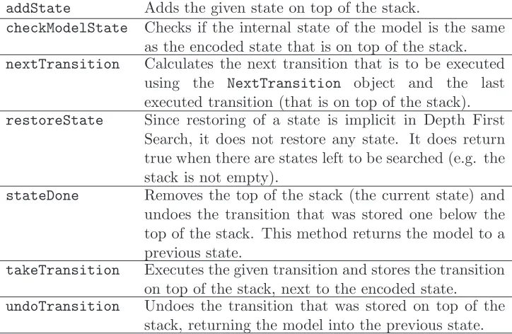
Table 4.1 shows how the abstract functions of the SearchAlgorithm are implemented for DFS.

4.2.4 Nested Depth First Search

For the cycle detection algorithm that is implemented in SpinJ _(acceptance

cycle detection), a nested depth first search is implemented. This algorithm is implemented as an extension of DepthFirstSearch. It is based on the algorithm as described on page 180 of [21].

There are two extra variables that need to be tracked during a nested depth first search:

toggle; to indicate that we are in the first or second search.

seed; that holds the state that initiated the nested search.

To make the nested search work, three parts have changed. First thetoggle

(31)

addState Adds the given state on top of the stack.

checkModelState Checks if the internal state of the model is the same

as the encoded state that is on top of the stack.

nextTransition Calculates the next transition that is to be executed

using the NextTransition object and the last executed transition (that is on top of the stack).

restoreState Since restoring of a state is implicit in Depth First

Search, it does not restore any state. It does return true when there are states left to be searched (e.g. the stack is not empty).

stateDone Removes the top of the stack (the current state) and

undoes the transition that was stored one below the top of the stack. This method returns the model to a previous state.

takeTransition Executes the given transition and stores the transition

on top of the stack, next to the encoded state.

undoTransition Undoes the transition that was stored on top of the

stack, returning the model into the previous state.

Table 4.1: The implementation description of the Depth First Search

restoreModel methods. This is not the most efficient method and a better

implementation is described on page 189 of [21]. There it is explained how each state needs only 1 extra bit to indicate if the nested search has encountered this state. This method is very hard to implement in the current design, because this would require some extra functionality of aStateStoreto store extra metadata with each state.

Secondly the nextTransition can return an extra transition when

conditionHoldsreturns true. When the model is in such a state where a nested

DFS needs to be started, this method will first return all normal transitions, and then the transition that starts the nested search. This special transition sets the toggle to true and encodes the current state of the model into the

seed.

The third change is to the takeTransitionfunction, which is responsible for executing the transition. If we are in the nested search (toggle is set to true), then some extra conditions are checked to see if a cycle has been detected. This occurs when we are in a state that is equal to theseedor if the state was already on the stack before theseed.

Acceptance cycle detection

Acceptance states are used to look for acceptance cycles in a state space. This is useful when checking for lifeness properties, which deals with infinite runs.

(32)

The acceptance cycle detection is implemented by theAcceptanceCycleSearch, which extends theNestedDepthFirstSearch. It implements theconditionHolds

method by checking if the current state of the model is an acceptance state.

4.2.5 Breadth First Search

Breadth First Search (BFS) is an alternative search algorithm that is implemented, which expands each state fully and per level of depth. This method is implemented using a Queue (see Figure4.1) to store the states that have to be expanded further. The Queue is implemented using a linked list of

State objects. Each of theseState objects remembers the following values:

The next state, which is needed for the single-linked list, which is how

these States are stored in the Queue.

Theprevious state, which references to the previous state in the executing

path (not a reference for the linked list).

Theencoded state, to be able to implement theSearchableStackinterface

(implementing the containsStatemethod).

The Transition identifier, to be able to write a trail-file when necessary.

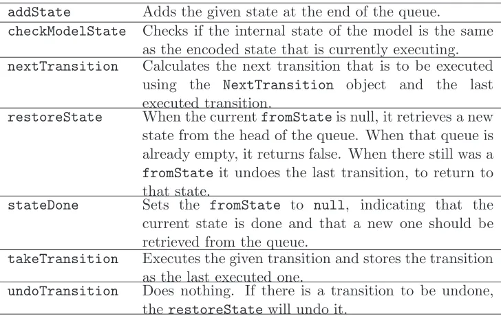
The abstract functions of the SearchAlgorithmthat are implemented for BFS are shown in table4.2. The Breadth First Search keeps track of the current state that is to be expanded, named fromState.

addState Adds the given state at the end of the queue.

checkModelState Checks if the internal state of the model is the same

as the encoded state that is currently executing.

nextTransition Calculates the next transition that is to be executed

using the NextTransition object and the last executed transition.

restoreState When the currentfromStateis null, it retrieves a new

state from the head of the queue. When that queue is already empty, it returns false. When there still was a

fromStateit undoes the last transition, to return to

that state.

stateDone Sets the fromState to null, indicating that the

current state is done and that a new one should be retrieved from the queue.

takeTransition Executes the given transition and stores the transition

as the last executed one.

undoTransition Does nothing. If there is a transition to be undone,

therestoreStatewill undo it.

(33)

4.2.6 The trail file

The trail file is created when the search algorithm finds an error. The file contains a list of identifier numbers to indicate which transition has been executed in which order. With these number the TrailSimulationcan easily execute that run again, to see in detail what went wrong.

Unfortunately, this trail file is not compatible with the trail files that are generated bySpin _{because the numbering of the transitions is done differently.}

4.3

Storage methods

To avoid expanding states that were already found during the search, states are stored using a StateStore. The StateStore’s only responsibility : Has this state been visited before? To answer this question, any implementation of the

StateStoreimplements the following methods:

addState tries to add the state to the store, but can return false when

the state has already been added.

getStoredreturns the number of states that have been stored successfully.

getBytes returns the number of bytes that is estimated to be used by

this storage facility.

The different storage methods can be split up in two categories: the exhaustive storage and approximate storage. Exhaustive storage will always provide the correct answer to the question stated above, but approximate can sometimes give a wrong answer. The can either be a false positive or a false negative.

A false negative occurs when a state was said to be visited before, while it has not been. When a storage method returns false negatives, some parts of the state space may never be reached. And while the state space was not completely checked, it can never be guaranteed that there is no error in the model.

A false positive occurs when a state was not visited before, while it has been. When a storage method returns false positive it possibly visits more states than necessary, thus slowing down the search algorithm.

The following sections will describe the different storage methods that are implemented in SpinJ_.

4.3.1 Hashtable

A hash table [18] is an exhaustive storage method that uses a set of “buckets”, which each can hold one or more states. A hash function is used - given a state as a key - to determine the identifier of the bucket where the state will be stored in.

(34)

Linked lists are used in the LinkedHashTable. Here every bucket is essentially a linked list (similar to theLinkedListprovided by the Java API), which is used to resolve any collisions. When two states both fall into the same bucket, they are stored in that linked list.

A disadvantage is that each item in the linked list requires an extra object, which costs 16 bytes of memory each. Also some CPU time is wasted, for creating the extra objects and traversing a linked list.

Arrays are used in theHashTableclass. In this implementation each bucket is an array of states (similar to the ArrayList provided by the Java API). Here we still have the advantage that handling collisions is simply adding a new state to that list, plus that the memory overhead is a lot smaller (only one extra object for each bucket).

When the array becomes too small we need to create a new array and copy all the items from the old array. This is still faster while we are adding states to the end of the list (as shown in [30]) than using a linked list.

Probing is an alternative solution to dealing with collisions. This method is implemented in theProbingHashTable. Every bucket in this hashtable contains simply one state and collisions are solved by finding a new bucket for that state. This removes almost all memory overhead of using lists (no extra objects used to store the bucket).

To find a next bucket, a new hash value must be calculated. This is done by rehashing, which is explained in more detail in Section 4.4.

The problem with a probing hash table is when the table becomes full, because then there will be a lot of collisions. In the current implementation this is solved having an overflow table, which gets used when an empty bucket could not be found.

4.3.2 Bitstate hashing

Bitstate storage is one of the first approximations for state storage that was added to Spin _[₂₀_{]. It works by storing only a variable number (}_k_{) of bits per}

state instead of storing the complete state. To determine which bits need to be set, k (preferably independent) hash functions are used to calculate k values. Each of these values then corresponds to an address in a table of bits.

To check if a state was already stored, all the values are calculated and those bits in the table are checked. Only when all bits are set, the model checker can conclude that the given state was visited before. This method can return a false negative when all the bits were already set by one or more other visited states that returned these hash values.

The implementation in SpinJ _{provides a} _{BitstateHashStore}_{class, which}

implements this algorithm using an array of long values (64-bits each). This way we can create a maximum array of 16 Gigabytes (64 bits * 231

(35)

4.3.3 Hash compaction

Hash compaction [40] is a storage method that is also an approximation. It is based on the idea that bitstate storage needs a very large table to work effectively (see [33]), so it simulates a very large table by storing the addresses of the bits that would be set in a bitstate table. These addresses can be stored in a normal hash table for efficient handling.

The implementation of the improved hash compaction algorithm (from [33])

inSpinJ _{is very straightforward. It uses a probing hash table to store the hash}

values instead of the states. First the value that needs to be stored is calculated by the first hash function. Then a second hash function is used to calculate the index of the bucket where the value will be stored.

The limitation of the current implementation of hash compaction is that it only supports table sizes that are a power of 2. Some optimisations from [12] are yet to be implemented, to make it possible to use tables of any size.

4.4

Hashing methods

A good hash function is important for all the storage methods that are described above. As Bob Jenkins describes on his website [28]: “A good hash function distributes hash values uniformly.”

A second requirement is that a good hash function must be as fast as possible. For example, MD4 is an excellent hash function with good distribution, but is much slower than some other functions.

Any class that implements the HashAlgorithm interface can be used as a hash function. TheHashAlgorithm interface declares a couple of functions to achieve this:

The hash(byte[], int) method takes a state (abyte[]) and an initial

value (an int) as parameters and calculates a 32-bits hash value for it.

Thehash(byte[], long)method takes a state (abyte[]) and an initial

value (an long) as parameters and calculates a 64-bits hash value for it.

The hash(byte[]) method takes a state (a byte[]) and returns a

HashGeneratorobject. This object makes it possible to generate a series

of 32-bits hash values (for example needed with a probing hash table).

The current version of SpinJ _{provides two implementations of the}

HashAlgorithm.

4.4.1 Jenkins hash

On his website [28], Bob Jenkins describes a very fast and good hash function, which is also used inSpin_{. The}_JenkinsHash_{class implements this algorithm.}

Also the rehashing optimisations from [12] are implemented here, but SpinJ

(36)

4.4.2 Hsieh hash

On his website [26], Paul Hsieh describes a method that is even faster than the one of Bob Jenkins describes and distributes the hash values almost as well. The problem with this method is that it is optimised for C code, where it can be compiled to only 13 assembly instructions per cycle. For this reason this new hash function is the default in Spin_{since version 5.}

The HsiehHash class implements this algorithm. Some small tests with a

(37)

Chapter 5

Abstract layer

As discussed in Section 3.2.2 the abstract layer provides an extension of the generic layer with the notion of concurrency. The concurrency within the model is based on the definition of one or more processes (also see Section3.2.2). Each of these processes can be seen as models by themselves, and the concurrent model as created by the Cartesian product of these.

In Figure 5.1 we can see the UML diagram that describes the relation between the different parts of this Abstract layer and how these are related to the Generic layer. The relation is mainly established through inheritance. Since the ConcurrentModelis an extension of the Model class, all algorithms that were defined in the Generic layer can just as easily be applied to any

ConcurrentModel.

5.1

Concurrent model

The ConcurrentModel has all the functionality of the Model class. To

accommodate the processes within a concurrent model, it defines two extra functions:

getNrProcesses() returns the number of processes that are currently

running inside the ConcurrentModel.

getProcess(index)returns the process that is located on the given index

(comparable with a list).

5.1.1 Processes

The processes that are running inside aConcurrentModelare implementations of theProcess class. Since every Process is an extension of the Model class, every process also can, e.g., determine the next transition (of that specific process) or check if a condition holds etc.

Next to this basic functionality, there are also two extra functions:

getId() returns the unique identifier of the process within the model.

This identifier is also the index that can be used in the getProcess()

(38)

Generic Layer Abstract Layer

spinj.concurrent.model

spinj.concurrent.search

ConcurrentModel<T: ConcurrentTransition>

+getNrProcesses(): int +getProcess(index: int): Process

ConcurrentTransition

+getProcess(): Process +isLocal(): boolean

Process<T: ConcurrentTransition>

+getId(): int

+onlyLocalTransitions(): boolean

spinj.model

Model<T: Transition>

+conditionHolds(condition: int): boolean +getName(): String

+nextTransition(last: T): T

Transition

+take() +undo() +getId(): int

+addMetaInfo(data: MetaInfo) +hasMetaInfo(data: MetaInfo): boolean

0..*

PartialOrderReduction<M: ConcurrentModel, T: ConcurrentTransition>

spinj.search

NextTransitionAlgorithm<M: Model<T>, T: Transition>

+next(model: M, last: T, stack: SearchableStack): T +duplicateState(model: M, last: T, state: byte[])

SearchAlgorithm<M: Model<T>, T: Transition>

1

Figure 5.1: An UML diagram that describes the Abstract layer ofSpinJ_{on top}

(39)

onlyLocalTransitions() returns true when all the current transitions

that may be executed from the current state of this process, only have local effects. This method can be used to limit the state space that has to be searched (see also Section 5.2).

5.1.2 Concurrent Transitions

The transitions that can be returned by Process.nextTransition() (and therefore also by the ConcurrentModel.nextTransition()) are always implementations of the ConcurrentTransition. This extension of the

Transitionclass defines two extra functions:

getProcess()returns the Processto which this transition belongs.

isLocal() returns true when this transition only has local effects (e.g.

not affecting other processes in the concurrent model).

These concurrent transitions can be used by optimisations techniques that require the knowledge of processes and their transitions (e.g. Partial Order Reduction, see Section5.2).

5.2

Partial Order Reduction

Partial order reduction [16] [13] is aimed at reducing the size of the total state space that needs to be generated. This algorithm changes the way the search algorithm can select the transitions that can be executed from a certain state. Instead of selecting all transitions that are enabled from the current state, we can choose a subset of that. So from a certain state s, we calculate

ample(s)⊆enabled(s), which will result in a reduced state space.

To determine theample(s), the similar heuristic is implemented as the one in [16]. First it returns only transitions from processes, for which all possible transitions only have a local effect. The conditions for when a transition only has a local effect is listed in [16], chapter 5. If at least one transition was found and no state was generated that was already on the stack, the algorithm ends (not returning any more transitions from other processes).

Partial order reduction is implemented in SpinJ _{as an extention of the}

NextTransitionclass, which is shown in the following listing.

1 public class PartialOrderReduction<M extends ConcurrentModel<T>, T

extends ConcurrentTransition<T>>

2 extends TransitionCalculator<M, T> { 3

4 public T next(final M model, T last) {

5 int i =model.getNrProcesses() − 1;

6 i f (last != null) {

7 Process<T>lastProc=last.getProcess() ;

8 i f (lastProc==null) {

9 return null;

(40)

11

12 T next=lastProc.nextTransition(last) ;

13 i f (next != null) {

14 next.copyMetaInfo(last) ;

15 return next;

16 } else i f (last.hasMetaInfo(MetaInfo.PartialOrderReduction)

17 && !last.hasMetaInfo(MetaInfo.StateOnStack) ) {

18 return null;

24 i f (last==null | | last.getProcess() .onlyLocalTransitions() ) {

25 while (i>= 0) {

26 final Process<T>proc=model.getProcess(i−−);

27 i f (proc.onlyLocalTransitions() ) {

28 T next =proc.nextTransition(null) ;

30 next.setMetaInfo(MetaInfo.PartialOrderReduction) ;

31 return next;

32 }

33 }

34 }

35 i=model.getNrProcesses() − 1;

36 }

37

38 while (i>= 0) {

39 final Process<T>proc =model.getProcess(i−−);

40 i f ( !proc.onlyLocalTransitions() ) {

41 T next =proc.nextTransition(null) ;

51 public void duplicateState(final M model, final T last, final byte[ ]

state,

52 final SearchableStack stack) {

53 i f (last.hasMetaInfo(MetaInfo.PartialOrderReduction) ) {

54 i f (stack.containsState(state) ) {

55 last.setMetaInfo(MetaInfo.StateOnStack) ;

56 }

57 }

58 }

59 }

(41)

PartialOrderReductionmeta info. When a state gets found that was visited before, then theduplicateStatefunction is called. This function checks if the last transition was a local one (by seeing if it has thePartialOrderReduction

meta info) and if the state was also on the stack. If this is the case, then the last transition also gets marked with the StateOnStackmeta info.

The implementation of thenextfunction to find the local processes consist of three parts. The first part on lines 6 to 22 determines if there was a previous transition, in which case we can try to find more transitions from that process. When there are no more transitions, then it checks if POR was used and there was no duplicate state on the stack. In that case it can return prematurely.

The second part (on lines 24 to 36) is when a next process must be found that is local. To see if a process is local, itsonlyLocalTransitionsfunction is called. The processes are scanned from the last on to the first, to mirror exactly howSpin_{executes its transitions.}

(42)

Chapter 6

Implementation of the

promela

language

As shown earlier in figures 3.2 and 3.3, the implementation of the promela

language consists of two parts: the promela _{compiler and the abstract}

promela _{model. The} promela _{compiler is responsible for generating the}

promela _{models that are implementations of the abstract}promela_model.

This chapter is going to explain these different parts. First it discussed the

promela _{language itself and how the compiler parses this language into an}

intermediate representation.

Then the second part will explain the tool layer, which contains abstract classes for a promela _{model, processes and transitions. Also there it will be}

explained what Java code is generated for the intermediate representation and how this relates to the tool layer.

The final section of the chapter will discuss some problems that were encountered while implementing the promela _{language in Java.} _These

problems are mostly caused by the differences between the C programming language and Java.

6.1

promela

This section explains thepromela_{language and how the compiler parses that}

language into the intermediate representation.

6.1.1 The language

From [1]: ”promela_{is a verification modelling language. It provides a vehicle}

for making abstractions of protocols (or distributed systems in general) that suppress details that are unrelated to process interaction. The intended use of

Spin _{is to verify fractions of process behaviour, that for one reason or another}

are considered suspect. The relevant behaviour is modelled in promela _and

verified. A complete verification is therefore typically performed in a series of steps, with the construction of increasingly detailed promela _{models. Each}

(43)

Listing 6.1: An example specification in thepromela_language.

1 chan com= [ 0 ] of {byte}; 2

3 int total;

4

5 active proctype counter() {

6 byte curr;

14 active proctype generator() {

15 byte cnt = 0;

28 active proctype monitor() {

29 do

30 : : assert(total< 16256) ;

31 od;

32 }

the environment (e.g., message loss, message duplications etc). Once the correctness of a model has been established withSpin_{, that fact can be used in}

the construction and verification of all subsequent models.

promela _{programs consist of} _{processes, message} _{channels, and} _variables.

Processes are global objects. Message channels and variables can be declared either globally or locally within a process. Processes specify behaviour, channels and global variables define the environment in which the processes run.”

For a list of features that is supported bySpinJ_{, see appendix}_C_.

To illustrate thepromela_{language, we will first explain the example model}

of Listing 6.1. At the top of this example, there are two global variables declared: a channel comand an integer total. Then there are three processes defined:

(44)

2. The generatorprocess, which generates numbers that are put into the

comchannel non-deterministically.

3. Themonitorprocess, which monitors if the totalvariable never exceeds 16256. When it does, the assertion fails and the model checker reports an error.

All three processes are declared active, meaning that one instance of the process is started when the model is initalized.

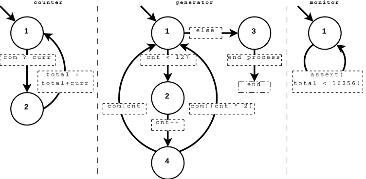
1

Figure 6.1: A graphical representation of the state in the three processes of the example from Listing 6.1.

The semantics of a Promela process is defined as a finite state automaton

(see 2.1.1). In Figure6.1the automata for the three processes are shown.

Let us look at thegeneratorprocess. State 1 of this process is the starting state (as with all processes), and there are two transitions possible from this state. This choice is a deterministic one, either thecntvariable is less than 127 and we go to state 2, or it is not and we go to state 3.

From state 2 there is only one transition executable, increasingcntvariable by 1. After state 4 there is again a choice, but this time a non-deterministic one. We can either send the value of cnt over the channel, or we can send twice that value over the channel. Also both end up back in the starting state, because of the do-loop.

The last transition that is shown, is the end processtransition. This one deletes the running process from the model and therefore does not end in any state. The other two processes are self-explanatory and will not be discussed further.

For more details on the promela _{language, see [}₂₁_{] and [}₁_{]. The rest of}

this section will explain how the compiler transforms a promela _{model (like}

(45)

spinj.promela.compiler

+BIT: VariableType = ("bit", "int", 1) +BOOL: VariableType = ("bit", "int", 1) +BYTE: VariableType = ("byte", "int", 8) +INT: VariableType = ("int", "int", 32) +MTYPE: VariableType = ("mtype", "int", 8) +PID: VariableType = ("pid", "int", 8) +SHORT: VariableType = ("short", "int", 16) +canConvert(type: VariableType): boolean

The abstract Action class is implemented by more classes: AssertAction, AssignAction, BreakAction, ChannelReadAction, ChannelWriteAction, ElseAction, ExprAction, OptionAction and PrintAction

Figure 6.2: An UML diagram that describes the intermediate representation of

(46)

6.1.2 The compiler

The design of the promela_{compiler was described earlier in Section}_3.3_{. The}

parser for this compiler was written in JavaCC and transforms the promela

code into the intermediate representation as described in the following section. The intermediate representation is a collection of Java objects describing the finite state automaton of the processes of thepromela_{model. These automata}

are optimised using the automaton optimizers, which will be described further on.

6.1.3 Intermediate representation

The intermediate representation of the promela _{code is a collection of}

Java objects describing the finite state automata of the processes of the

promela _{model. These different types of objects are shown in Figure} _6.2_.

The main object that represents the complete promela _{specification is the}

Specification object. This object holds the global variables as well as the

processes that are described here.

The processes are represented by Proctype objects. These objects are responsible for storing the local variables that are declared within the