Computational Study of Multi Phase Flows Using Lattice Boltzmann Model

(1)

page 1

Computational Study of Multi-Phase Flows Using Lattice Boltzmann Model

Saeed J. Almalowi

1

_{, Dennis E. Oztekin}

2

_{, Alparslan Oztekin}

3

1

_{Corresponding author, Mechanical Engineering Department, Taibah University, Almadianh Almunwwarah, KSA}

2

_{Mechanical Engineering, Georgia Institute of Tech., GA 30332, USA}

3

_{Mechanical Engineering and Mechanics, Lehigh University, PA 18015, USA}

---*---Abstract -**

The Multi-Relaxation Time Lattice

Boltzmann method has been employed to investigate the behavior of droplets in fluid. A density distribution function has been introduced for each fluid and was utilized to simulate the dynamics of the droplets and the velocity field of each phase. Buoyancy and other interactive forces between phases are modeled to predict the evolution of droplets as they are rising. A fully periodic domain is employed in this study and the result is a transient flow simulation of a multi-phase immiscible fluid for geometries ranging from a single droplet case to a case with four adjacent droplets. Also studied here is the interaction between the droplets and the no-slip boundary. The evolution of the droplets and the transient flow field around it are examined when droplets are placed on the no-slip surface initially. The breaking up of the droplet is predicted for different arrangements.

Key Words:

Lattice Boltzmann, Droplet Dynamics,

Bubbles, Boundary Interaction, Interactive Forces

1. Introduction

The present study investigates the nonlinear dynamics that arise when droplet of light fluid rise though a heavier fluid. The Lattice Boltzmann method is utilized to study this multiphase flow. In their classical review paper on the field Chen and Doolen (1998) identified multiphase flows as an area which Lattice Boltzmann methods exceled at. The present investigators have since demonstrated that the method is an effective way to model and study complex multiphase flows (see Almalowi and Oztekin 2014, Almalowi et al. 2013a). Cheng et al.(2010) published a powerful paper which demonstrated that bubble dynamics is a field which is perfect for the application of Lattice Boltzmann. In the present study, the temporal and spatial characteristics of the flow resulting from the rise of a light fluid droplet in a heavier fluid will be studied. Then results obtained from our model will be compared to well-known

regimes in bubble dynamics. After validating the model by such methods, more interesting flows, such as the interactions between multiple bubbles and the interactions between bubbles and a solid boundary will be studied. In the present study, the Shan and Chen method, as outlined in their paper (see Shan and Chen 1993), is employed to incorporate the interactive forces between the two liquids present into the Lattice Boltzmann Method. Velocity, vorticity and pressure fields induced by the rising droplets are examined for various arrangements of droplets.

2. Mathematical Model

The Lattice Boltzmann Method is grounded in kinetic theory. The original theory comes from the Boltzmann equation

∂f

∂t

+ 𝐜 ⋅ ∇f = (

∂f

∂t

)

_collision

(1)

Here, equation (1) has been simplified so as to remove the effects of external forces. The distribution function,

f

, is a function of position, x; time, t; and the fluid velocity c. f represents the number of particles present at a specific time and position which have a velocity in the neighborhood of u. The term at the right side of equation (1) determines the time rate of change of

f

due to collision. In the 1950s Bhatnagar et al. (1954) introduced the approximation:

(

∂f

∂t

)

_colision

=

f

eq

− f

τ

(2)

Here feq is the equilibrium value of f and τ is the lattice relaxation time. For the single relaxation time method τ is described below in terms of lattice viscosity.

τ = 3ν + 0.5 (3)

(2)

page 2

ν =

δ

t

δ

_x2

1 R

_e

(4)

[image:2.595.314.500.304.367.2]

Notice that, just like real kinematic viscosity, the units are length squared per unit time, because Reynolds number is dimensionless. It can be assumed for the remainder of this paper that all variables with dimensions have been discretized in terms of the lattice discretization parameters. While on the topic of discretization, it seems prudent to discuss the discretization used in the following derivations. In LBM research the lattice studied is typically described by the shorthand DnQm; where n is the number of spatial dimensions and m is the number of lattice direction as each node. Demonstrated in Figure 1 is a in the D2Q9 arrangement, which was used in the present investigation. Once the lattice arrangement is chosen, a number of important parameters can be worked out. The “lattice velocity”,

𝐞

𝐤, is the expression for the discrete velocity along each lattice branch, k. For the arrangement shown in Figure 1:

ek=c{(0,0),(0,1),(1,0),(0,-1),(-1,0),(1,1),(1,-1),(-1,-1,(-1,1) } (5) Where c = │c│ is the lattice speed, which is simply

δ

x

⁄

δ

t. The weighting function is also determined once the arrangement is selected. For this arrangement

w

k

= 1/36{16, 4, 4, 4, 4, 1, 1, 1, 1} (6)

Figure 1. D2Q9 lattice arrangement

From equations 1 and 2, the single relaxation time governing equation, the evolution equation, can be shown to be:

f

_k

(𝐱 + 𝐞

_𝐤

δ

_t

, t + δ

_t

) = f

_k

(𝐱, t) (1 −

δt

τ

) +

δt

τ

f

k

eq

_{(𝐱, t) (7)}

This is, of course, an explicit method. At each time step fk

is

determined from the previous value of

f

_k and the updated value of fkeq. The equilibrium value of

f

is an important parameter because it is used to force the conservation laws. The Chapman-Enskog expansion developed in Chapman

and Cowling (1999), is used as the base for the equilibrium distribution function. Here it is with the first three terms, which is all that is needed here:

f

_keq

= C {1 + C

₁

𝐞

_𝐤

+ C

₂

[(𝐞

_𝐤

⋅ 𝐮)

2

₋

1

2 |𝐮|

2

_]

+ ⋯ } (8)

where

𝐮

is the fluid velocity. Now these three general constants (C,

C

₁,

C

₂) are used to force the three constraints from kinetic theory:

∑ f

k k

= ρ

and

∑ f

k k

𝐞

𝐤

= ρu

(9)

It has been shown in He and Lou (1997) that these constraints will force the evolution equation to satisfy the Navier-Stokes equation. Solving for the three general constants using these constraints gives;

f

_keq

= ρw

_k

{1 + (3

𝐞

𝐤

⋅ 𝐮

c

2

+

9

2 (𝐞

_𝐤

⋅ 𝐮)

c

4

2

−

3

2 |𝐮|

2

c

2

)} (10)

LBM has shown itself to be very adept at modeling multiphase flows as shown by Hou et al. (1997). It completely avoids the hassle of interface tracking which slows down classical methods. To deal with multiple fluids

simply introduce multiple density distribution

functions:

f

_k𝜎, with

σ = {1 … j}

where

j

is the number of fluids in the system. Now the evolution equation becomes the system of equations:

f

_kσ

(𝐱 + 𝐞

𝐤

δ

t

, t + δ

t

) − f

kσ

(𝐱, t) = −

δt

τσ

[f

kσ

(𝐱, t) −

f

_kσeq

(𝐱, t)]

(11)

As it is, this evolution equation is missing a key component to multiphase flows, inter-particle forces,

𝐅

int. To add this effect into our model we used the model introduced by Shan and Chen (1993). As was mentioned earlier:

∑ f

_kσ

= ρ

σ

k and

∑ f

_kσ

_𝐞

𝐤

= ρ

σ

𝐮

σ

k

(12)

Now we also need a common velocity which can be found by what is effectively mass averaging:

𝐮

σ

=

∑

ρσ𝐮σ τσ j σ=1 ∑ ρσ τσ j σ=1

(13)

With this we can solve for an equilibrium velocity. Using this velocity in the calculations for

f

_k𝜎𝑒𝑞will automatically account for the inter-particle forces as demonstrated in Shan and Chen (1993).

ρ

σ

𝐮

𝛔𝐞𝐪

= ρ

σ

𝐮

𝛔

+ τ

σ

𝐅

σ

(14)

𝑓1 𝑓5

(3)

page 3

Here

𝐅

σ is the total inter-particle force on fluid

σ

per unit

volume, but it has been shown by Huang et al. (2009) that

𝐅

σ_{can be extended to include other forces such as body} forces and adhesion forces. In the present investigation adhesion forces were ignored; however, a body force, gravity, was included. This was necessary since, modeling of a rise of a lighter fluid droplet in a heavier fluid requires a body force in the opposite direction to a density gradient. Therefore, in the present investigation

𝐅

σ

= 𝐅

_intσ

+ 𝐅

_bodyσ

(15)

The inter-particle force is calculated using an interaction potential function:

𝜑(𝑥, 𝑥

′

) = G

σσ̅

_{(𝐱, 𝐱}

′

_)ψ

σ

_(𝐱)ψ

σ̅

_(𝐱

′

_{) (16)}

Where x and

𝐱

′ are the position vectors of any two points in the flow domain and

ψ

σis the mass density function. The function

G

σσ̅

(𝐱, 𝐱

′

₎

_{is a Green’s function. Here only} interactions between a point in the fluid and the adjacent point are considered so

G

σσ̅

(𝐱, 𝐱

′

₎

_{reduces too:}

G

σσ̅

_{(𝐱, 𝐱}

′

_{) = {}

0, |𝐱 − 𝐱′| > 𝑐

G, |𝐱 − 𝐱′| ≤ c

(17)

where G is a constant parameter which controls the strength of the inter-particle forces. Now that the effecting area is in the immediate neighborhood, the general position variable,

𝐱

′,is reduced to xk which is the position vector for the nodes next to x in the direction of k. With the interaction potential known and

G

σσ̅

_{(𝐱, 𝐱}

′

₎

_{defined in such a simple} way, the interactive force becomes:

𝐅

_intσ

(𝐱) =

−ψ

σ

(𝐱) ∑

_𝜎𝑗_̅=1

G

σσ̅

(𝐱, 𝐱

𝐤

) ∑

m_k=1

w

_𝑘

ψ

σ̅

(𝐱

𝐤

)(𝐱

𝐤

−

𝐱) (18)

Now all that remains is to calculate the effective mass which is:

ψ

σ

= ρ

₀σ

(1 − e

−ρσ⁄ρ0σ

_{) (19)}

𝜌

₀𝜎is the constant density of incompressible fluid

𝜎

. The gravity force is much simpler:

𝐅

_bodyσ

= 𝐠ρ

σ

₍₂₀₎

For the sake of presentation a coloring step can be added to this method in the two fluid cases.

The idea is to create a function κ which is one at a node entirely dominated by the lighter fluid, negative one at a node entirely dominated by the heavier fluid, and somewhere between one and negative one for a node which consists of both the light and heavy fluid.

κ =

ρ

light

_{− ρ}

heavy

ρ

light

_{+ ρ}

heavy

(21)

At any given instant this coloring function can be contour plotted to produce an image showing where each fluid is.

The standard single relaxation time LBM discussed above is known to have stability issues at the high speed flows that can be seen in the kinds of multiphase flow studied here; especially when the density differences grow larger. To deal with these issues Multi Relaxation Time Lattice Boltzmann Method (MRTLBM) was developed. Consider the vector equation:

𝐟(𝐱 + 𝐞

k

δ

t

, t + δ

t

) − 𝐟(𝐱, t)

= S[𝐟(𝐱, t) − 𝐟

eq

(𝐱, t)] (22)

Here

f

_k and fkeq have been rewritten as

f

and

f

eqwhich are vectors of dimension k. Notice that when the collision matrix is defined as

S =

δt

τ

I (23)

Where I is the identity matrix, the equation reduces to the single relaxation time LBM evolution equation. The idea in MRTLBM is to convert the right hand side of this equation from velocity space to moment space using the linear mapping:

m = M. f (24)

Then defining,

Ŝ = M ∙ S ∙ M

−1 the evolution equation becomes:

f

_k

(𝐱 + 𝐞

𝐤

δ

t

, t + δ

t

) − f

k

(𝐱, t) =

−M

−1

Ŝ[m

_k

(𝐱, t) − m

_keq

(𝐱, t)] (25)

For a more detailed derivation see the work of d’Humieres and his colleagues (see d’Humieres et al. 2002 and d’Humieres 1992).

In the present study the moment transformation matrix and the equilibrium moment are selected as

(4)

page 4

and m

eq

=

[

ρ

−2ρ + 3(J

_x2

+ J

_y2

)

ρ − 3(J

_x2

_{− J}

y

2

₎

J

_x

−J

x

J

_y

−J

_y

(J

_x2

_{− J}

y2

)

J

x

J

y

]

(27)

where Jx and Jy are linear momentum in x and y directions. Components of the diagonal matrix

Ŝ

are 1, 1.4, 1.4, 1, 1.2, 1, 1.2, 1/ω and 1/ω.MRTLBM has been successfully applied by the present authors on other flow problems in the past (see Almolawi et al. 2014, Almolawi and Oztekin 2012 and Amolawi et al. 2013b).

In the present investigation a mass conserving boundary contention treatment similar to the one studied by Zou and He (1997) and Kuo and Chen (2008) is employed. The idea in this method is to derive the three directions facing away from the boundary from the set of equations formed by: the conservation of mass, the conservation of momentum (equation (9)), and the non-equilibrium bounce back condition. The non-equilibrium bounce back condition states that the part of the density distribution function not contributing to the equilibrium will be reflected from the boundary. Therefore:

f

_a

− f

_aeq

= f

_b

− f

_beq

(28)

where the direction b is opposite of a. In the no slip no penetration case shown this generates:

f

₁

= f

₃;

f

₅

= f

₇

−

1

2

(f

2

− f

4

)

; and

f

8

= f

6

+

1

2

(f

2

−

f

4

) (29)

The stream function, and vorticity field, ω, are determined using the definition:

ω =

∂v

∂x

−

∂u

∂y and

ω = −∇

2

_{Φ (30)}

Equation (29) can be utilized to calculate stream function and the vorticity field from the discretely solved velocity field. Central differencing for the lattices at the interior domain and backward or forward differencing at the lattices on the boundary are used to discretize equation (29). Resulting in a discretized set of coupled equations which are solved using Jacobi iteration.

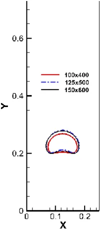
With all other parameters held constant, the shape of the droplet at its terminal velocity is determined for three different grid sizes, 100x400, 125x500, and 150x600. Due to the nature of the Lattice Boltzmann Method, as the grid size is varied the time step must be adapted hence this test represents both spectral and temporal convergence. Figure 2 depicts the shape of the droplet as it reaches its terminal

[image:4.595.380.482.218.449.2]

speed. The shape of the droplet is plotted at t = 0.6 sec. While there exists a discernible difference in the shape predicted between 100x400 and 125x500 cases; the difference becomes negligible between the 125x500 and 150x600 cases. This ensures that spectral and temporal convergence attained by the grid size of 150x600, as such, this is the grid size used in the present study. Using this grid size and the given lattice velocity the corresponding time step is derived to be 0.00015s.

Figure 2.The shape of the droplet plotted at t=0.60s for various grid sizes

The droplet’s dynamics is determined by the following dimensionless groups:

Re =

ρUd

μ

, EO =

ρgd

2

λ

and MO =

gμ

4

∆ρ

ρ

2

_λ

5

(31)

(5)

page 5

Doolen 2002)

𝐏

𝛔

=

ρ

σ

3 +

G(ѱ

σ

₎

2

6 (32)

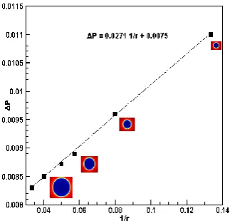
[image:5.595.247.534.83.563.2]

Figure 3 shows the results of the bubble test conducted for various radii of the droplet. The pressure difference between the two fluids is plotted against 1/r and the slope of the curve yields the surface tension which is calculated to be 0.027.

Figure 3. Pressure difference between inside and outside of the droplet as a function of 1/r for G =1.6

In order to validate the model employed by the present study, simulations for a single droplet rising in an infinite fluid are conducted for two different set cases each with different Re and EO. The evolution of the droplets of these two cases is shown in Figure 4. For the first case (Re = 2.88 and EO = 27.8) the oblate ellipsoid shape is attained as the terminal speed is reached. For the second case (Re = 11.32 and EO = 54.4) the spherical cap is predicted as depicted in Figure 4. These two cases are determined by the initial size of the droplet (d = 25for the first case and d = 35for the second case) as the interactive forces are kept the same for both cases. The flow regime and the shape of the droplet agree well with those reported by Gupta and Kumar (2008). The terminal speed of the rising droplet will be attained as the drag force and the interactive forces exerted on the droplet are balanced. Figure 4 also show the speed of the droplet for Re = 11.32 and EO = 54.4 as a function of the dimensionless time, T = t(g/d)1/2. The terminal speed agrees very well with correlations documented earlier (see Gupta and Kumar 2008, Viana et al. 2003, Davies and Taylor 1950 and Rodriguez 2001).

a) _b)

c)

Figure 4. The shape of the single droplet in an infinite fluid for a) Re = 2.88 and EO = 27.8 and b) Re = 11.32 and EO = 54.4. The images are taken at time 0.1s, 0.6s, 0.8s, 2.5s, 3.8s, and 4.0 s. c) The speed of the droplet vs dimensionless time. The symbols in (c) is prediction by the present study and the dashed line is the result of correlations reported previously

[image:5.595.43.205.222.377.2]

(6)

page 6

velocity field. It represents the droplet rising in an infinite

fluid. The oblate ellipsoid is attained as the droplet reaches to the terminal speed. In density images shown below, red color denotes the higher density fluid while blue color denotes the lower density fluid. For the time steps and the spacing between the lattices selected in the present simulations, the relaxation frequency, inverse of relaxation time, for lighter fluid is ω1=0.5657 and for the heavier fluid (water) is ω2=1.0 with inter-particle amplitude is G=1.6The density ratio of fluids is 1.2 and the Atwood number, A=𝜌ℎ−𝜌𝑙

𝜌ℎ+𝜌𝑙

~0.1

where

𝜌

ℎ and

𝜌

𝑙 are densities of the heavier and the lighter fluids, respectively. The rising droplet induces a flow in both fluids as shown in Figure 5a and b. The location of the droplet is imposed on the contour of the stream function to better illustrate how the flow filed is induced by rise of the droplet. The complex flow field is present in the vicinity of the droplet with the presence of small and large scale recirculating vortices. They dissipate quickly away from the droplet. Larger pressure gradient is present at the front side of the droplet as shown in Figure 5d.

a) _b)

c) d)

Figure 5. a) Density contour, b) stream function, c) vorticity and d) pressure field for a single droplet rising in an infinite fluid. Images are shown at t = 1.16s

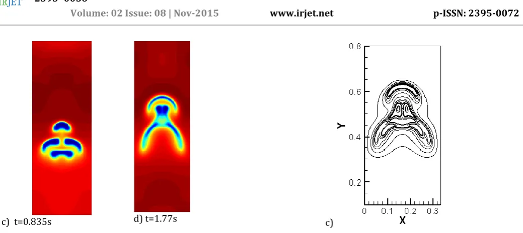
Figure 6 depicts the evolution of four droplets in an infinite medium. The shape and the dynamics of each droplet are influenced significantly by the presence of the other droplets in the field. The initial shape and the configuration of the droplets are illustrated in Figure 6a. The top droplet assumes nearly the shape of the oblate ellipsoid and remains unattached from the other droplets at all times, as shown here. However, its shape is still influenced by the other droplets. The droplets in the middle show a quite complicated evolution. Their leading edge gets closer to each other and merges at the later stages of the flow. Their trailing edge separates and coalescences with the droplet which was located at the bottom initially, as shown in Figure 6c and 6d.

[image:6.595.313.537.85.316.2]

(7)

page 7

c) t=0.835s d) t=1.77s

Figure 6. Density contours at various times

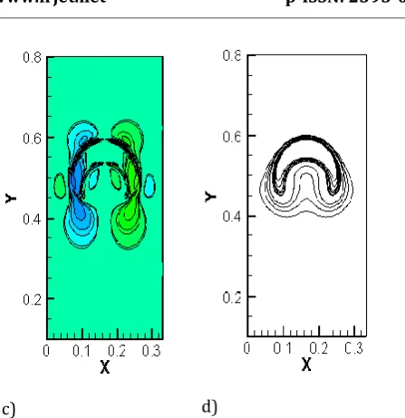
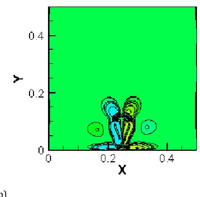
Figure7shows the flow field near the four rising droplets in an infinite fluid at t = 1.47s.The density contour and the streamlines are shown together in Figure 6a. Complex flow field around the droplets is obvious from these images. Both the intensity of the vortices and the pressure gradient induced by the rising droplets decay fast away from the droplet.

a) b)

c)

Figure 7. a) Stream function, b) vorticity and c) pressure field for four droplets rising in an infinite fluid. Images are shown at t = 1.47s

a)t=0s b) t=0.340s _{c ) t= 0.660s}

d) t = 1.88s e) t = 2.103s f) t = 2.663s

[image:7.595.40.560.70.302.2]

(8)

page 8

Figure 8 shows the density contours of a single droplet at

various times. Initially, the droplet is placed on the no-slip bottom boundary and the initial shape of the droplet is semi-circle. The no-slip boundary condition is also applied at the top boundary while periodic conditions are applied at the side boundaries. Again the droplet is lighter than the fluid around it. The droplet starts rising and it is elongated in the direction of gravity. At the early stages it is still attached to the boundary, but as time progress it develops a filament connecting the droplet to the no-slip surface. This filament is stretched and eventually breaks up. As the unattached droplet rises in the heavier fluid the residue of the droplet sticks to the surface. The buoyancy force is not strong enough to lift the residue of the droplet away from the surface so the residue remains on the surface. The influence of the no-slip boundary on the evolution of the droplet is very strong as seen in Figure 8.

The instantaneous streamlines and the vorticity contours are depicted, in Figure 9, for a single droplet that is initially placed on the no-slip boundary at time, t = 1.174s. The interface separating the droplet from the heavier fluid is also shown on the contours of the stream function. Two counter rotating vortices cover both the droplet and the heavier fluid. Another pair of weaker counter rotating vortices at each side of the droplet is also present. The intensity of the flow is much stronger near the droplet as the flow is induced by rising droplet. The fluid away from the droplet is undisturbed as shown both by flow and the vorticity field.

a)

b)

Figure 9. a) Stream function and b) vorticity field for a semi-circled shaped droplet initially placed on the no-slip boundary. Contours are shown at t = 1.174s.

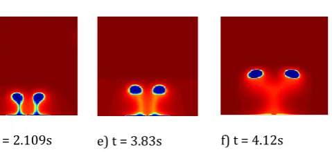
Figure 10 shows the density contours of two droplets at various times. Initially, the semi circled shape droplets are placed on a no-slip bottom boundary. Periodic boundary conditions are imposed at the side boundaries and the top boundary is a no-slip and no-penetration surface. The droplets move away from each other as rise. At time, t=2.1s, the droplets are attached to the surface by a thin filament, as seen in Figure 10d. At later stages of the flow, both droplets are unattached from the surface and still move away from each other. Even later stage of the flow, the residue remains on the no-slip surface and spreads itself over the surface while the unattached droplets rise further into the heavier fluid as seen in Figure 10f. Again the no-slip surface strongly influences the development of the droplet and the flow induced by the rising droplet.

[image:8.595.316.516.108.304.2]

(9)

page 9

d) t = 2.109s

e) t = 3.83s f) t = 4.12s

Figure 10. Density contour of two single semi-circle shaped droplets that are placed on the no-slip boundary. Images are taken at various times.

Instantaneous streamlines and the vorticity contours are shown in Figure 11 for the two droplet case discussed above at the time, t=4.12s. The location of the droplets is imbedded on the contours of the stream function; helping to relate the induced flow field to the rising droplets. The presence of several counter rotating vortex pairs and their interaction with the no-slip boundaries are creating a very complicated flow field around the rising droplets.

a)

[image:9.595.57.297.99.209.2]

b)

Figure 11. a) Stream function and b) vorticity field for two semi-circled shaped droplets initially placed on the no-slip boundary. Contours are shown at t = 4.12s.

4. Conclusion

Multi-Relaxation Time Lattice Boltzmann method is implemented to study lighter droplets rising in a heavier fluid. Both an infinite and bounded fluid domains are considered. Density distribution functions for each fluid and the function for the coloring step to identify the location of interface separating each immiscible fluid is determined at various stages. The evolution of the rising droplet and the temporal and spatial characteristics of the flow induced by such motion are examined for various arrangements. The present method is validated by comparing our results against well-known regimes in droplet dynamics. Interactions between multiple bubbles and the interactions between bubbles and a solid boundary are illustrated. These interactions create a complicated velocity, vorticity and the pressure field in the vicinity of rising droplets. It is also illustrated here how droplets rise when they are placed on the no-slip boundary initially. First, bubbles from a long thin filament and at a later stage of evolution the filament breaks and bubble dis-attach from the boundary. As the residue of the droplet spreads over the no-slip surface dis-attached droplet continue to rise away from the surface. This study proves that Lattice Boltzmann method could be an effective computational fluid dynamics (CFD) tool to simulate multi-phase flows with interfaces evolving with complex fashion.

Acknowledgement

The authors would like to acknowledge the support of Saudi government for the scholarship provided for SJA.

[image:9.595.50.241.388.570.2]

(10)

page 10

[1]. Almalowi, S.J. and Oztekin, D.E., 2014, Rayleigh-Taylor

Instability Studied with Multi-relaxation Lattice Boltzmann Method, J. Mechanics Engineering and Automation, 4(5) 365-371

[2]. Almolawi, S.J., Öztekin, D.E. and Öztekin, A., 2014, Numerical Simulations of Lid-Driven Cavity Flows using Multi-relaxation Time Lattice Boltzmann Method, Engineering Applications of Computational Fluid Dynamics (Advanced Structured Materials)vol44, edited by: Shaari, K., Zlati, K. and Mokhtar, A. Springer

[3]. Almalowi, S.J., Oztekin, D.E. and Oztekin, A., 2013a, Rayleigh-Taylor Instability Studied with Multi-relaxation Lattice Boltzmann Method., ASME Conference Proceeding IMECE

[4]. Almolawi, S.J., Öztekin, D.E. and Öztekin, A., 2013b, Regularized Multi-relaxation Time lattice Boltzmann Method for Flow Past Square Cylinders, Computers and Fluids (under review)

[5]. Almolawi, S.J. and Öztekin, A., 2012, Flow Simulations using Thermal Lattice Boltzmann Method, Journal of

Applied Mathematics,

http://dx.doi.org/10.1155/2012/135173

[6]. Bhatnagar, P.L., Gross, E.P. and Krook, M., 1954, A Model for Collision Processes in Gases. I. Small Amplitude Processes in Charged and Neutral One-Component Systems, Physical Review, 94(3), 511-525

[7]. Chapman, S. and Cowling, T.G., 1999, The Mathematical Theory of Non-Uniform Gases, Digital Edition, Cambridge Mathematical Library

[8]. Chen, S. and Doolen, G.D., 1998, Lattice Boltzmann Method for Fluid Flows,Annu. Rev. Fluid Mech,30,329-364 [9]. Cheng, M., Hua, J. and Lou, J., 2010, Simulation of Bubble-Bubble Interaction Using a Lattice Boltzmann Method, Computers & Fluids, 39, 260-270

[10]. Davies, R.M. and Taylor, G.I., 1950, The Mechanics of Large Bubbles Rising Through Extended Liquids in Tube, Proceeding of the Royal Society, 200, No.1062

[11]. d’Humieres, D., Ginzburg, I., Krafczyk, M., Lallemand, P. and Luo, L., 2002, Multiple-Relaxation-Time Lattice Boltzmann Models in Three Dimensions, Philosophical Transactions Royal Society of London A¸360, 437-451 [12]. d’Humieres, D., 1992, Generalized Lattice Boltzmann Equations, Rarefied Gas Dynamics Theory and Simulations, 159,450-458

[13]. Gupta, A. and Kumar, R., 2008, Lattice Boltzmann Simuulation to Study Multiple Bubble Dynamics,Int. J. of Heat and Mass Transfer, 51,5192-5203

[14]. He, X. and Doolen, G.D., 2002, Thermodynamic Foundation of Kinetic Theory and Lattice Boltzmann Models for Multiphase Flows, Journal of Statistical Physics, 107, 309-328

[15]. He, X. and Luo, L., 1997, Lattice Boltzmann Model for the Incompressible Navier-Stokes Equation, Journal of Statistical Physics, 88(3), 927-944

[16]. Hou, S., Shan, X., Zou, Q., Doolen, G.D. and Soll, W.E., 1997, Evaluation of Two Lattice Boltzmann Models for Multiphase Flows, Journal of Computational Physics, 138, 695-713

[17]. Huang, H., Li, Z., Lui, S. and Lu, Z., 2009, Shan-and-Chen-type Multiphase Lattice Boltzmann Study of Viscous Coupling Effects for Two-Phase Flow in Porous Media, International Journal for Numerical Methods in Fluids, 61, 341-354

[18]. Kuo, L.S. and Chen, P.H., 2008, A Unified Approach for Nonslip and Slip Boundary Conditions in the Lattice Boltzmann Method, Computers & Fluids, 38, 883-887 [19]. Kuzmin, A. and Mohamad, A.A., 2010, Multirange Multi-relaxation Time Shan-Chen Model with Extended

Equilibrium, Computers and Mathematics with

Applications, 59, 2260-2270

[20]. Rodriguez, D., 2001, Generalized Correlation for Bubble Motion. AIChE J, 47, No. 47, 39–44

[21]. Shan, X. and Chen, H., 1993, Lattice Boltzmann Model for Simulating Flows with Multiple Phases and Components, Physical Review E., 47(3), 1815-1819 [22]. Succi, S., 2001, The Lattice Boltzmann Equation for Fluid Dynamics and Beyond, Oxford Science Publications [23]. Viana, F., Pardo, R., Yanez, R., Tallero, J.L. and Joseph, D.D., 2003, Universal Correlation for the Rise Velocity of Long Gas Bubbles in Round Pipes, J. Fuid Mech., 494, 379– 398

[24]. Zou, Q. and He, X., 1997, On Pressure and Velocity Boundary Conditions for the Lattice Boltzmann BGK Model, Physics of Fluids, 9, 1591

Biographies

(11)

page 11

Mr. Dennis Oztekin

PhD Student at Georgia Tech, GA 30332-0405, USA- College of Engineering, The George W. Woodruff School of Mechanical Engineering

Prof. Alparslan Oztekin, PhD Professor at Lehigh University-Bethlehem, Packard laboratory, PA18015, USA-

Mechanical Engineering and

Computational Study of Multi Phase Flows Using Lattice Boltzmann Model

page 1