FCM BPSO: ENERGY EFFICIENT TASK BASED LOAD BALANCING IN CLOUD COMPUTING

(1)

ISSN: 1992-8645 www.jatit.org E-ISSN: 1817-3195

265

COMPARISON OF THINNING ALGORITHMS FOR

VECTORIZATION OF ENGINEERING DRAWINGS

MATÚŠ GRAMBLIČKA1, JOZEF VASKÝ1

1

Ph.D. student, Slovak University of Technology in Bratislava Faculty of Materials Science and

Technology in Trnava, Paulínska 16, 917 24 Trnava, Slovak Republic

2

Assoc. Prof., Slovak University of Technology in Bratislava Faculty of Materials Science and Technology

in Trnava, Paulínska 16, 917 24 Trnava, Slovak Republic

E-mail: [email protected], [email protected]

ABSTRACT

The thinning algorithms are used for creation the skeleton of an object. The thinned image consists of the lines one pixel wide. The thinning or skeletonization reduces the image complexity. The thinning process is widely used in vectorization based on the thinning methods. In this contribution is presented the comparison of nine known iterative parallel thinning algorithms with one proposed and their performance evaluation on sets of the engineering drawings. The results are evaluated and compared in regard to suitability to vectorization of the engineering drawings.

Keywords:Thinning Algorithm, Skeleton, Vectorization, Engineering Drawing

1. INTRODUCTION

The vectorization is transformation process of the raster image consisting of pixels to vector representation consisting of vectors. The vectorization methods can be very roughly divided into two groups, thinning and non-thinning vectorization methods. Vectorization methods based on thinning yield better results in terms of the line geometry, but natively do not preserve line width. In this paper it is examined ten thinning algorithms on the set of engineering drawings and evaluated which algorithms are most suitable for the further vectorization of these drawings. The motivation of this paper is to find the most accurate thinning algorithms for the purposes of engineering drawings vectorization. The contribution of this article is the proposed thinning algorithm that is derived from precedent thinning algorithms to serve for specific vectorization purposes.

Thinning or skeletonization is technique commonly used in raster vector conversion [1], [2], [3], [4]. Thinning is the process of identifying the skeleton of an object. The thinned version of a shape is called the skeleton. The skeleton is basically a central line extraction of an object, resulting from thinning [5], [6]. A skeleton captures essential topology and shape information of an object in a simple form [7]. Thinning is a very

important preprocessing step for the analysis and recognition of different types of images. Thinning techniques can be divided into two groups. The first group is based on an iterative thinning of the original image using the boundary erosion process [6]. All thinning algorithms used in this paper belong to this group. The iterative process removes pixels while sequence of pixels one pixel wide remains. The second group of thinning techniques is based on distance transform [8] to compute the skeleton of an object. The iterative approaches need more passes before attaining the final result, so the computing time can be higher [9]. They are also sensitive to presence of a noise. The second category of approaches based on the distance transform gives results more efficiently. Works [10], [11] for instance use this second thinning approach.

(2)

266 Skeletons are important shape descriptors in object representation and recognition.

A skeleton is very useful in the fields such as a 3D generation from 2D image, 3D model matching and retrieval, medical image analysis [7], bubble-chamber image analysis, text and handwriting recognition and analysis. The representation with the thin lines is more suitable for an extraction of the endpoints, the connecting points and the connections between the components [12].

The thinning is also a key step of the preprocessing in many systems of the pattern recognition. In the OCR applications an extraction process usually follows the thinning process. Thinning also plays an important role in reducing data complexity for the vectorization of the raster line drawings such as electrical circuit diagrams, maps and architectural blueprints, mechanical and technical drawings [13] and for the recognition of characters and the other objects [14].

The thinning algorithms have good accuracy of the line location however they tend to add a number of hooks, when the image is not regular. Moreover, the thinning algorithms are poor in terms of correct positioning of the junctions and the end points. The original line width recovery is straightforward using the methods based on distance transform, but not using an iterative thinning [15]. Thinning usually introduces incorrect connecting points. Short branches connected through these connection points can deform the shape of the skeleton and oppose further recognition and vectorization [16]. The frequent access to the pixels at iterative thinning slows the rate of a vectorization [17].

A good thinning algorithm should accomplish the following requirements: maintaining connectivity of the skeleton, producing one pixel wide skeleton, to be resistive to the noise, and time efficient. The reasons and need for a thinning of the images can be formulated as:

a) Reduction of the amount of data required to be processed.

b) Reduction of the time required to process the pattern.

c) Shape analysis can be made more easily on the thinned pattern.

The thinning algorithms can be classified [18], [19], [20]:

• Iterative (pixel based) o _Sequential o _Parallel

• Non-Iterative (non-pixel based) o _{Medial axis transform}

o _{Line following} o _Other

2. ITERATIVE PARALLEL THINNING

ALGORITHMS

All tested thinning algorithms in this paper are iterative parallel algorithms. Whether the pixels will be deleted in nth iteration depends in parallel thinning on the result from the previous (n-1)th iteration. Values of the pixels and its neighbors at the (n-1)th iteration determine the values of the pixels at the next nth iteration. Parallel thinning algorithms usually use a 3*3 matrix that represents neighborhood around the examined pixel as shown in table 1.

Table 1 Matrix 3x3 Represents 8-neighboorhood Of Pixel P1

P9 P2 P3 P8 P1 P4 P7 P6 P5

(3)

267 The examples of other specific thinning algorithms used for thinning the raster images that are not tested in this paper may be mentioned Rosenfeld's parallel algorithm used in the vectorization application AutoTrace, Voronoi diagrams, Wang Zhang and Holt thinning algorithms. As the examples of the newer algorithms these works can be mentioned [32], [33], [34], [35].

For the purposes of iterative parallel thinning algorithms let´s propose matrix 3x3 and define the three functions B(P), A(P) and C(P).

B(P1) represents the number of non-zero neighbors of P1. It is computed as:

B(P1) = P2+P3+...+P9.

[image:3.612.92.301.337.392.2]

A(P1) represents the number of 0,1 patterns in the sequence P2, P3, P4, P5, P6, P7, P8, P9, P2. Examples of these functions can be seen on fig 1.

Figure 1 Example Of Functions B(P1), A(P1): a) B(p1) = 2 , A(p1) = 1; b) B(p1) = 2, A(p1) = 2

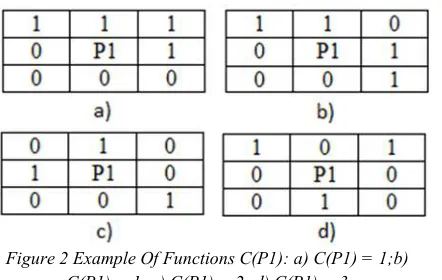
The function C(P) is connectivity number. C(P1) function is little harder to understand so fig. 2 is proposed. C(P1) is the number of distinct 8-connected components count in the neighborhood of the pixel P1. One of the ways how to compute function C(P1) can be:

C(P1) = !P2 Λ (P3 V P4) + !P4 Λ (P5 V P6) + !P6 Λ (P7 V P8) + !P8 Λ (P9 V P2).

Figure 2 Example Of Functions C(P1): a) C(P1) = 1;b) C(P1) = 1; c) C(P1) = 2; d) C(P1) = 3

The Guo hall and Stentiford thinning algorithms use the function C(P).

Zhang Suen Thinning Algorithm

Zhang Suen thinning algorithm [22] (ZS) is fast parallel thinning algorithm with two sub-iterations. The conditions used in the first sub-iteration in order to remove the south-east pixel are:

1. 2 ≤ B(P1) ≤ 6 2. A(P1) = 1 3. P2 Λ P4 Λ P6 = 0 4. P4 Λ P6 Λ P8 = 0

In the second sub-iteration conditions in steps 3 and 4 change, in order to remove the north-west pixels:

3. P2 Λ P4 Λ P8 = 0 4. P2 Λ P6 Λ P8 = 0

End points [36] and pixel connectivity should be preserved [18]. Issue with that algorithm is that with the presence of a noise near north-east and south-west corners these are extended instead of deleted [19].

Lu Wang Thinning Algorithm

The algorithm proposed by Lu and Wang [23] (LW) to solve problem of diagonal lines occurring in ZS algorithm. It is derivative of ZS. The only difference from ZS algorithm is that the first condition is replaced by condition: All pixels whose number of value is 1 in 8-neighborhood is in the range 3 to 6.

LW algorithm should shrink horizontal lines well, but does not get one pixel wide skeleton in sloping lines [37].

Modified Thinning Algorithm

Zhang and Wang [38] proposed Modified algorithm (MA). It uses slightly extended neighborhood as shown in table 2. Point P1 can be deleted if all conditions are met:

1. 2 ≤ B(P1) ≤ 6 2. A(P1) = 1

3. (P2*P4*P8 = 0) or P11 = 1 4. (P2*P4*P6 = 0) or P15 = 1

MA should be faster than ZS [38].

Table 2 Neighborhood Of Pixel P1 In Algorithm MA P10 P11 P12 P13

P9 P2 P3 P14

P8 P1 P4 P15

P7 P6 P5 P16

Kwon Woong Kang Thinning Algorithm

[image:3.612.91.312.534.674.2]

(4)

268 It is a two pass algorithm. On the image the first pass criterions are applied and then on the result the second pass criterions further produced the final skeleton.

In the Pass 1 steps one and two are the same as in ZS algorithm, expect that the step 2 uses condition that number of value 1 in 8-neighbour pixels are in the range 3 to 6 instead of 2 to 6.

In the second pass conditions are:

1. P9 = 1 Λ P8 = 1 Λ P6 = 1 Λ P3 = 0 2. P3 = 1 Λ P4 = 1 Λ P6 = 1 Λ P9 = 0 3. P5 = 1 Λ P6 = 1 Λ P8 = 1 Λ P3 = 0 4. P4 = 1 Λ P6 = 1 Λ P7 = 1 Λ P9 = 0

It can get the 1-pixel wide lines, handles the end point preserving and perfect 8-connectivity [37].

Hilditch Thinning Algorithm

Hilditch algorithm [39], [40] presented by Naccache and Shinghal, provides good results when thin the image edges [35]. Hilditch algorithm consists of four conditions before deleting the pixel:

1. 2 ≤ B(P1) ≤ 6 2. A(P1) = 1

3. (P2 Λ P4 Λ P8 = 0) or A(P2) != 1 4. (P2 Λ P4 Λ P6 = 0) or A(P4) != 1

Hilditch algorithm does not work on all patterns. For example, it removes staircase patterns almost completely.

Guo Hall Thinning Algorithm

Algorithm proposed by Guo and Hall [30] (GH) is two sub-iteration parallel thinning algorithm. The GH gives thinner skeletons than ZS and LW algorithms.

In that algorithm new function N(P) is introduces. It allows to preserve the end points as well as to remove redundant pixels. The function NP is defined:

N(P) = Min(N1(P1), N2(P1)); where

N1(P1) = (P9 V P2) Λ (P3 V P4) Λ (P5 V P6) Λ (P7 V P8)

N2(P1) = (P2 V P3) Λ (P4 V P5) Λ (P6 V P7) Λ (P8 V P9)

An edge point will be deleted if it satisfies these conditions:

1. C(P1) = l 2. 2 ≤ N(P1) ≤ 3

3. Then apply one of the following depending of the iteration:

a) (P2 V P3 V P5) Λ P4 = 0 in odd iterations; or b) (P6 V P7 V P9) Λ P8 = 0 in even iterations

Condition 1 preserves local connectivity that means the deletion of pixel P1 does not break the connectivity and guarantees that pixel P1 is not a break point [18]. Condition 3(a) deletes north-east pixels and 3(b) deletes south-west pixels [19]. The GH algorithm detects the end points better than the ZS algorithm [18].

Stentiford Thinning Algorithm

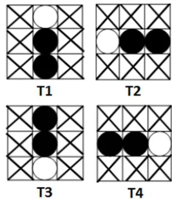
Stentiford and Mortimer proposed algorithm [41] that uses four templates for decision to remove pixels as shown at fig 3. White circle represents white pixel, black circle black pixel and the crossed squares means that on these pixels does not matter. Algorithm can be proposed with four sub-iterations. First and second conditions for pixel deletion are the same for all four sub-iterations:

1. B(P1) > 1 2. C(P1) = l

3. It is looked for pixel location where pixels match those in template T1.

[image:4.612.329.500.396.594.2]

In the next sub-iterations the only difference is that it is used next template T2 until T4. The algorithm repeats until there are no more pixels to delete.

Figure 3 Four Templates Used In The Stentiford Thinning Algorithm

Arabic Parallel Thinning Algorithm

Arabic thinning algorithm [42] uses four sub-iterations that are divided into 4 conditions. A dark point P1 is set for deletion if one of each sub-iteration is true. First and second conditions are the same for all sub-iterations:

(5)

269 First sub-iteration

3. P2 Λ P4 Λ P6 = 0 4. P4 Λ P6 Λ P8 = 0 Second sub-iteration 3. P2 Λ P6 Λ P8 = 0 4. P4 Λ P6 Λ P8 = 0 Third sub-iteration 3. P2 Λ P4 Λ P8 = 0 4. P2 Λ P6 Λ P8 = 0 Fourth sub-iteration 3. P2 Λ P4 Λ P6 = 0 4. P2 Λ P4 Λ P8 = 0

Efficient Parallel Thinning Algorithm

Aparajeya and Sanyal proposed another parallel thinning algorithm [43]. There are 2 sub-iterations, the pixel deletion criterions are:

First sub-iteration

1. !P4 Λ P8 Λ ((P2 Λ !P5 Λ !P6) V (!P2 Λ !P3 Λ P6)) or

2. P6 Λ P7 Λ P8 Λ ((P9 Λ P2 Λ !P4) V (!P2 Λ P4 Λ P5)) or

3. !P2 Λ !P3 Λ !P4 Λ (((!P5 Λ !P6 Λ P8) Λ (P9 V P7)) V ((!P9 Λ P6 Λ !P8) Λ (P7 V P5))) = 1 Second sub-iteration

1. P4 Λ !P8 Λ ((!P9 Λ !P2 Λ P6) V (P2 Λ !P6 Λ !P7)) or

2. P2 Λ P3 Λ P4 Λ ((P5 Λ P6 Λ !P8) V (P9 Λ !P6 Λ P8)) or

3. !P6 Λ !P7 Λ !P8 Λ (((!P9 Λ !P2 Λ P4) Λ (P5 V P3)) V ((P2 Λ !P4 Λ !P5) Λ (P3 V P9))) = 1

This algorithm is the enhancement of the GH algorithm. The connectivity number is no longer computed. The algorithm provides good results if the input image is not very noisy.

Proposed Thinning Algorithm

The proposed algorithm has three passes where first two passes are identical with those in KWK algorithm. In the third pass the algorithm uses 5x5 neighborhood, table 3, and aims to delete corner pixels which do not form structure but are secondary thinning product of previous two passes.

In the third pass there are four sub-iterations with conditions:

1. P11 = 0 Λ P2 = 1 Λ P4 = 1 Λ P15 = 0 Λ P7 = 0 2. P15 = 0 Λ P4 = 1 Λ P6 = 1 Λ P19 = 0 Λ P9 = 0 3. P19 = 0 Λ P6 = 1 Λ P8 = 1 Λ P23 = 0 Λ P3 = 0 4. P23 = 0 Λ P8 = 1 Λ P2 = 1 Λ P11 = 0 Λ P5 = 0

Table 3 Matrix 5x5 Represents 8-neighboorhood Of Pixel P1 In Proposed Thinning Algorithm

P26 P10 P11 P12 P13

P24 P9 P2 P3 P14

P23 P8 P1 P4 P15

P22 P7 P6 P5 P16

P21 P20 P19 P18 P17

The first sub-iteration deletes south west corners. The second sub-iteration deletes north west corners. The third sub-iteration deletes north east corners and the fourth sub-iteration deletes south east corners.

3. METHOD

The thinning algorithms are evaluated on the set of real engineering drawings. As was mentioned before, good thinning algorithm should maintain connectivity of skeleton, produce one pixel wide skeleton, be resistive to noise, and time-efficient. Based on these requirements five qualities are measured: connectivity, thinning ratio, thinness, sensitivity and execution time. These metrics are chose because every of them can be computed using exact mathematical equation and that they address directly to requirements setting by this paper. The maintaining of a skeleton connectivity is associated with the connectivity number which represents number of unique points on a skeleton after the thinning. The reduction rate and thinness metrics are indirectly used for specify how thin the skeleton is. However whether the thinning algorithm produces one pixel wide skeleton is not possible to judge from the results of these two metrics but skeleton observation is also needed. In this paper the sensitivity metric is associated with the requirement of resistance to noise. The execution time represents how much time is needed to yield a skeleton thus how the thinning algorithm is time-efficient.

Connectivity

The original image and the skeleton in an ideal case should have the same amount of the discrete points and the end points. In reality thinned image would have more of these elements. More of these points in favor to the skeleton reflect more disconnection. The equation 1 [44] expresses that relationship.

C ∑ 1

1 2

0

where size = width * height of the image in pixels. Formula B(Pi) < 2 can be understood that pixel is

(6)

270 value that is closer to value of the original image denotes more quality skeleton.

Reduction rate

The reduction rate expresses the rate of pixel reduction of the original image expressed as a percentage. The value of this reduction can be computed by equation 2.

1 ∗ 100% 2

where Tt is the number of pixels in the thinned

image, To is the number of pixels in the original

image.

Higher the reduction rate value means higher amount of pixels that were deleted from the original image.

Thinness

The thinness of a skeleton can be computed by the equation 3 inspired by the work of Zhou, Quek and Ng [44]. It expresses that the skeleton which is not one pixel wide contains triangles composed of three black pixels around pixel Pi.

" 1 ∑&%'(%)* # $%

+,-. / 01#,# 3# 4567_/9 3

Th Pi Pi ∗ P9 ∗ P2 ? Pi ∗ P9 ∗ P8 ? Pi ∗ P8 ∗ P7 ? Pi ∗ P7 ∗ P6 ? Pi ∗ P6 ∗ P5

? Pi ∗ P5 ∗ P4 ? Pi ∗ P4 ∗ P3 ? Pi ∗ P3 ∗ P2

The thinness value that is nearer to 1 suggests thinner skeleton.

Sensitivity

The noise that is presented in the image can cause a deformation of the skeleton. The pixels that remained after thinning process as a product of noise can be difficult to recognize comparing to normal pixels. The total number of the cross points that remained after thinning should be good indicator of sensitivity thus the resistance to the noise. The cross point can be defined as a point that connect three or more branches. The sensitivity can be measured by equation 4 in this paper.

∑ 4

1 F G 2

0

Formula A(Pi) > 2 can be understood as the

number of branches outgoing from the pixel Pi.

Lower sensitivity value thus the lesser amount of cross points means better sensitivity of the algorithm and better skeleton.

Execution time

The execution time is the time duration of the thinning operation. The time is started to record with the beginning of the actual thinning process until the end of the process. One algorithm is executed several times and the average time is the execution time.

4. RESULTS

The thinning algorithms were implemented in C# programming language. All tests were performed in Windows operating system under Oracle virtual machine with 4 GB dedicated memory on the processor Intel i5 4670K.

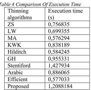
[image:6.612.348.507.328.485.2]

The table 4 represents the comparison of the execution time. MA, Hilditch and Efficient are the three fastest thinning algorithms. The Stentiford and proposed thinning algorithms are the two slowest one. All algorithms except Stentiford and proposed perform under one second.

Table 4 Comparison Of Execution Time Thinning

algorithms

Execution time (s)

ZS 0,756835

LW 0,699355

MA 0,576294

KWK 0,838189

Hilditch 0,584245

GH 0,955331

Stentiford 1,427934 Arabic 0,886065 Efficient 0,577033 Proposed 1,2088184

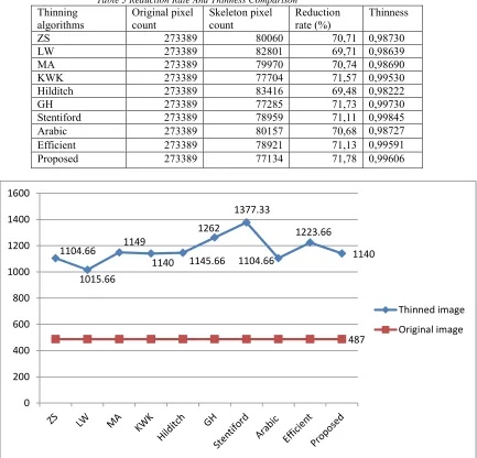
The table 5 represents the reduction rate and the thinness comparison of the thinning algorithms. The highest reduction rate is obtained by proposed algorithm with the third highest thinness value. The second highest reduction rate is attained by GH algorithm which also gets second highest thinness value. The KWK, Stentiford and Efficient algorithms get very good results in relation to reduction rate and thinness. Hilditch algorithm reaches the lowest reduction rate as well as the thinness value. The average reduction rate is 70,86% (69,48 – 71,78).

(7)

271 is the highest. These values express that there is more disconnection and more cross points after Stentiford thinning. On the contrary LW algorithm attains the closest connectivity value to original but second lowest reduction rate and thinness values. The sensitivity remains in the mid-range. It means

[image:7.612.90.523.185.601.2]

that there is more connectivity at the expense of thinness. The Arabic thinning algorithm has solid connectivity and sensitivity results but the thinness is not so high. The most balanced algorithms in relation to thinness, connectivity and sensitivity are KWK and proposed algorithms.

Table 5 Reduction Rate And Thinness Comparison Thinning

algorithms

Original pixel count

Skeleton pixel count

Reduction rate (%)

Thinness

ZS 273389 80060 70,71 0,98730

LW 273389 82801 69,71 0,98639

MA 273389 79970 70,74 0,98690

KWK 273389 77704 71,57 0,99530

Hilditch 273389 83416 69,48 0,98222

GH 273389 77285 71,73 0,99730

Stentiford 273389 78959 71,11 0,99845

Arabic 273389 80157 70,68 0,98727

Efficient 273389 78921 71,13 0,99591

Proposed 273389 77134 71,78 0,99606

Graph 1 Connectivity Comparison. Lower Value Is Better 1104.66

1015.66 1149

1140 1145.66 1262

1377.33

1104.66

1223.66

1140

487

0 200 400 600 800 1000 1200 1400 1600

Thinned image

(8)

272

Graph 2 Sensitivity Comparison. Lower Value Is Better

Based on the observation and the comparison of the thinned skeletons some findings can be concluded. Overall, the produced skeletons of engineering drawings are approximately same with small but important variations. ZW, LW, MA, Hilditch and Arabic thinning algorithms tend to produce double diagonal lines while KWK, GH, Stentiford, Efficient and proposed do not. KWK, MA, Arabic, Hilditch, proposed and ZW algorithms produce less spurs and hooks than other algorithms.

5. CONCLUSION

In this paper ten thinning algorithms were tested in order to examine their suitability for the further vectorization of the engineering drawings. In general all tested thinning algorithms were able to thin the engineering drawings to the level applicable for the vectorization. Since ZW, LW, MA, Hilditch and Arabic thinning algorithms remain double diagonal lines they appear to be less suitable for vectorization than KWK, GH, Stentiford, Efficient and proposed algorithms. From these five algorithms KWK and proposed produce less amount of the spurs and the hooks, have a better connectivity and therefore they appear as the most suitable thinning algorithms among the others for the vectorization of the engineering drawings. The proposed algorithm was derived from KWK algorithm to reduce corners pixels so it even more softens the skeleton structure which is beneficial for

the vectorization process. The drawback of the proposed algorithm is his slowness.

The best two algorithms for vectorization are KWK and proposed because of its most balanced results. Although whichever the algorithm would be utilize to thin the engineering drawings in order to vectorize them after the vectorization certain processes have to be used for recover lost connectivity and for adjusting geometry e.g. the gap filling and the polygonal approximation. The vectorization process is simpler if there are fewer pixels on skeleton. In case of deletion some pixels which should not be deleted, the gap filling should be used after the vectorization and the polygonal approximation for ablation the aberrations caused by the thinning

6.

DISCUSSION

This study confirmed some previous findings of the literature. As is posted in work [37] LW algorithm was not able to get one pixel wide skeleton in diagonal lines. Results confirmed that MA is faster than ZS as is shown in work [38]. KWK got one pixel wide diagonal lines as stated in the paper [19]. As posted in work [15], using the iterative thinning algorithms the original line width was lost. The line width is one of the main attribute of line in the engineering drawings.

The issues identified by this study are the number of hooks and spurs that still remain at resulted 776.33

901.33

821

915.66

809.66 1029.66

1087.33

784.66 926

917

251.33

0 200 400 600 800 1000 1200

Thinned image

(9)

273 skeletons. The question is whether to develop more accurate thinning algorithm that prevent from their origin or remove these artifacts in the postprocessing steps.

The limitations of the current work are that the resulted skeletons are not vectorized and that only the parallel thinning algorithms were compared. The proposed future work should vectorize these individual skeletons and evaluate which thinning algorithm yields the most accurate skeleton for the purposes of the engineering drawings vectorization. The preserving of the line width should also be one of the future works.

ACKNOWLEDGEMENT

This publication is the result of implementation of the project: "UNIVERSITY SCIENTIFIC PARK: CAMPUS MTF STU - CAMBO" (ITMS: 26220220179) supported by the Research & Development Operational Program funded by the EFRR.

REFERENCES:

[1] R.D.T. Janssen and A.M. Vossepoel, Adaptive Vectorization of Line Drawing Images, Computer Vision and Image Understanding, vol. 65, no. 1, pp. 38-56, 1997.

[2] Kasturi R, Bow ST, El-Masri W, Shah J, Gattiker JR, Mokate UB (1990) A system for interpretation of line drawings. IEEE Trans Pattern Anal Mach Intell 12(10):978–992. [3] E. Bodansky and M. Pilouk, “Using Local

Deviations of Vectorization to Enhance the Performance of Raster-to-Vector Conversion Systems,” Int’l J. Document Analysis and Recognition, vol. 3, no. 2, p. 67-72, Dec. 2000. [4] V. Nagasamy and N.A. Langrana,

“Engineering Drawing Processing and Vectorization System,” Computer Vision, Graphics and Image Processing, vol. 49, no. 3, pp. 379-397, 1990.

[5] Girija Dharmaraj. Algorithms for Automatic Vectorization of Scanned Maps. THE

UNIVERSITY OF CALGARY.

DEPARTMENT OF GEOMATICS

ENGINEERING. CALGARY, ALBERTA. JULY, 2005.

[6] Lam, L., Lee, S.W., Suen, C.Y, 1992. Thinning Methodologies- A Comprehensive Survey, IEEE Transactions on Pattern Analysis and Machine Intelligence 14(9), 869-885.

[7] Lakshmi, J. K., Punithavalli, M. A Survey on Skeletons in Digital Image Processing. Proceeding ICDIP '09 Proceedings of the International Conference on Digital Image Processing, pages 260-269, IEEE Computer Society Washington, DC, USA, 2009. ISBN:

978-0-7695-3565-4, doi

10.1109/ICDIP.2009.21.

[8] Niblack C.W., Gibbons P.B., Capson D.W. (1992) Generating skeletons and centerlines from the distance transform. CVGIP: Graph Models Image Process 54(5):420–437.

[9] Tombre, K., Tabbone., S., 2000. Vectorization in Graphics Recognition: To Thin or not to Thin, International Conference on Pattern Recognition (ICPR’00)- 2, Barcelona, Spain [10] X. Hilaire and K. Tombre, “Robust and

Accurate Vectorization of Line Drawings,” IEEE Trans. Pattern Analysis and Machine Intelligence, vol. 28, no. 6, pp. 890-904, June 2006.

[11] Kolesnikov AN, Belekhov VV, Chalenko IO (1996) Vectorization of raster images. Pattern Recognit Image Anal 6(4):786–794.

[12] J.Y. Chiang et al., A New Algorithm for Line Image Vectorization, Pattern Recognition, vol. 31, no. 10, pp. 1541-1549, 1998.

[13] Xu, X. W., Bai, Y. B., 2000. Computerising Scanned Engineering Documents, Computers In Industry 42(2000), p. 59-71.

[14] Lopich, A., Dudek, P. "Hardware implementation of skeletonization algorithm for parallel asynchronous image processing", journal of signal processing system, July 2009. [15] Llados, J., Rusinol, M. Handbook of Document

Image Processing and Recognition. Springer-Verlag London. Editors: Doermann, D., Tombre, K. kapitola Graphics Recognition Techniques. Pages 489-521. 2014. ISBN 978-0-85729-858-4. DOI 10.1007/978-0-85729-859-1.

[16] S. J. Tue and John Y. Chiang, The archiving of line drawing images, Proc. SPIE, SPIE’s Photonics East’95 Sympo.Conf.on Digital Image Storage and Archiving Systems, Philadelphia, PA, USA, Vol. 2606, pp. 145– 156 (1995).

(10)

274 [18] Kumar, H. Kaur, P. A Comparative Study of

Iterative Thinning Algorithms for BMP Images / (IJCSIT) International Journal of Computer Science and Information Technologies, Vol. 2 (5) , 2011, 2375-2379.

[19] Jagna, A. Some algorithms for image thinning using spatial domain processing. Jawaharlal Nehru Technological University, India, 2012. URI: http://hdl.handle.net/10603/3466.

[20] E. Hastings. A Survey of Thinning Methodologies, Pattern analysis and Machine Intelligence, IEEE Transactions, vol. 4, Issue 9, 1992, pp. 869-885.

[21] Blum, H. A transformation for extracting new descriptors of shape, in Proc. Symp. Models for the Perception of Speech and Visual Form, Cambridge, MA: MIT Press. 1964.

[22] Zhang, T. Y., Suen, C. Y. A fast parallel algorithm for thinning digital patterns, Comm. ACM, vol. 27, no. 3, pp. 236-239. 1984. [23] Lu, H.E., Wang, P.S.P. A Comment on “A Fast

Parallel Algorithm for Thinning Digital Patterns”, comm. AMC, vol.29, no. 3, pp.239-242. 1986.

[24] Wang, P. S. P. Hui, L., Fleming, Jr. T. Further improved fast parallel thinning algorithm for digital Patterns. Proceedings of Computer Vision, Image Processing and Communication Systems and Applications, 1986, pp. 37-40. [25] Holt, C. M., Stewart, A., Clint, M., Perrott, R.

H. An improved parallel thinning algorithm, Comm. ACM, 1987, vol. 30, no. 2, pp. 156-160.

[26] Se Hyun Park, Sang Kyoon Kim and Hang Joo Kim. A Fully Parallel Thinning Algorithm using a Weighted Template, IEEE, Tenco-Digital signal proce. pp. 1996. No. 300-303. [27] Kwon, J. S, Woong J., Kang, E. K. An

Enhanced Thinning Algorithm Using Parallel Processing, IEEE, pp.no.752-755. 2001. [28] Ahmad and Ward,2002,“A Rotation Invariant

Rule-Based Thinning Algorithm for Character Recognition”, IEEE, Trans. Patt.Anal.Machine Intll.,Dec,Vol. 24.No.12. pp. 1672-1678. [29] Rockett, P. I. An Improved Rotation- Invariant

Thinning Algorithm, IEEE, Trans. Patt.Anal.Machine Intll., Oct 2005, Vol. 27.No.10. pp. 1671-1674.

[30] Guo, Z. Hall, R., W. Parallel thinning with two-subiteration algorithms, Comm. ACM, vol. 32, no. 3, pp. 359-373. 1989.

[31] Zhang, F., Wang, Y., Gao, Ch., Si, S., Xu, J. An Improved parallel thinning algorithm with two subiterations, Optoelectronics Letters,4(1), Jan.2008, 69-71.

[32] Gulshan Goyal, Maitreyee Dutta, Akshay Girdhar, “A Parallel Thinning Algorithm for Numeral Pattern Images in BMP Format”, International Journal of Advanced Engineering & Application, Jan. 2010, pp. 197-202

[33] Jia Liang. A Research on Guided Thinning Algorithm and Its Implementation by Using C#. International Journal of Image Processing (IJIP), Volume (5) : Issue (5) : 2011 580. 2011. [34] Abu-Ain, W. et al. and col. Skeletonization

Algorithm for Binary Images. The 4th International Conference on Electrical Engineering and Informatics (ICEEI 2013). [35] Thulasi, S., S. Jyothi, R., L. A Novel Image

Thinning Method for Signature Recognition System. Department of Computer Science and Engineering, College of Engineering Karunagappally. 2016.

[36] Subashini P., Jansi S. Optimal Thinning Algorithm for detection of FCD in MRI Images. International Journal of Scientific & Engineering Research Volume 2, Issue 9, September-2011 1 ISSN 2229-5518.

[37] Devi, H.K.A., (2006). Thinning: A Preprocessing Technique for an OCR System for the Brahmi Script. Ancient Asia. 1, pp.167– 172. DOI: http://doi.org/10.5334/aa.06114. [38] Zhang, Y. Y.; Wang P. S. P. A modified

parallel thinning algorithm. Pattern Recognition, 1988., 9th International Conference on Year: 1988 Pages: 1023 - 1025 vol.2, DOI: 10.1109/ICPR.1988.28429. [39] Naccache, N., J. Shinghal, R. An investigation

into the skeletonization approach of Hilditch. Journal Pattern Recognition archive Volume 17 Issue 3, 1984 Pages 279-284. doi>10.1016/0031-3203(84)90077-3

[40] Widiarti, A., R. “Comparing Hilditch, Rosenfeld, ZhangSuen, and Nagendraprasad -Wang-Gupta Thinning”, International Scholarly and Scientific Research & Innovation, Vol:5, 2011.

[41] Stentiford, F., W., M., Mortimer, R., G. Some New Heuristics for Thinning Binary Handprinted Characters for OCR, R.G. 1 IEEE Transactions on Systems, Man, and Cybernetics, SMC-13 (1983), p. 81.

(11)

275 [43] Aparajeya, P., Sanyal, S. AN EFFICIENT

PARALLEL THINNING ALGORITHM

USING ONE AND

TWOSUB-ITERATIONS.12th IASTED International Conference on Computer Graphics and Imaging (CGIM-2011).