RULES REDUCTION AND OPTIMIZATION OF FUZZY LOGIC MEMBERSHIP FUNCTIONS FOR INDUCTION MOTOR SPEED CONTROLLER

5070

HAND WRITTEN CHARCTER RECOGNITION USING

NEURAL NETWORK AND DEEP BELIEF NETWORK

1_{MAJID HAMEED KHALAF,} 2_{BELAL AL-KHATEEB,} 3_{RABAH NORY FARHAN}

1_{Msc. student, Department of ComputerScience, College of ComputerScience and}

Information Technology, University of Anbar, Ramadi, Iraq

2_{Assistant Professor, Department of ComputerScience, College of ComputerScience and}

Information Technology, University of Anbar, Ramadi, Iraq

3_{Assistant Professor, Department of ComputerScience, College of ComputerScience and}

Information Technology, University of Anbar, Ramadi, Iraq

E-mail: 1_{[email protected],} 2_{[email protected],}3_{[email protected]}

ABSTRACT

In this paper a comparison is done between two classification architectures, those are Standard Neural Networks (NN) that contain one hidden layer and Deep Learning concept using Deep Belief Networks (DBN). Both algorithms are applied on Capital English Character with same architectures and parameter for comparison purpose. The Standard Neural Network was trained as a supervised learning using Back Propagation (BP) algorithms while Deep Belief Network was trained using two phases of learning, the first phase as unsupervised learning using Contrastive Divergence (CD) algorithm and the second phase as a supervised learning using Back Propagation algorithms for fine tuning the network. Each character represented as an image in grayscale pixels. The features are extracted depending on the intensity of pixel in image that white color represents as a 0’s and black color represent as a 1’s. DBN is represented as a stack of Restricted Boltzmann Machines (RBM). The DBN learning procedure undergoes a pre-training stage and a fine-tuning stage. DBN gave a higher performance as compared with the Standard neural networks with an accuracy of approximately 92.3% for a classification of Capital English handwritten characters.

Keywords: Backpropagation, Supervised Learning, Contrastive Divergence, Character Recognition, Deep Belief Networks.

1. INTRODUCTION

Machine learning is widely used to solve practical problems by learning from a given input. The center qualities of machine learning are to keep a good representation of data and create a generalized algorithm to predict inconspicuous information appropriately [1]. Deep learning (DL) is a branch of machine learning in light of an arrangement of calculations that endeavor to model abnormal state reflections in information by utilizing model designs, with complex structures or something else, made out of multiple non-linear transformations [2][3]. Deep of the architecture indicates to the number of phases of arrangement of non-linear operations in the service learned [4]. Deep learning permits computational models that are made out of numerous preparing layers to learn representations of information with various levels of deliberation.

These methods have significantly improved the state-of-the-art in speech recognition, visual object recognition, object detection and many other domains such as drug discovery and genomics [1][5]. Facebook is also planning to empower its big data with deep learning methods to make predictions about its users. Deep learning finds complex structure in large data sets by using the backpropagation algorithm to describe how a machine should change its internal parameters that are used to calculate the representation in each layer from the representation in the previous layer [5].

ISSN: 1992-8645 www.jatit.org E-ISSN: 1817-3195

5071 unsupervised learning use unlabeled data [3,5]. In this paper, we are focusing to comparing between Standard Neural Network and Deep Belief Network approaches to solve a classification problem of recognizing Capital English Characters.

2. RELATED WORKS

The main problems of computer vision is the image classification that is concerned with determining the visual structures of an input image. The ability of object recognition system using the neural networks in some particular tasks like digit recognition, face recognition is claimed to be near to human performance.

Geoffrey E. Hinton, Simon Osindero, Yee-Whye (2006) introduced how to use the complementary priors to remove the explaining way impact that makes difficult deduction in violently connected belief nets with many hidden layers. They used complementary priors and proposed a fast greedy algorithm. It can train deep learning belief networks in a one by one layer for each time. The fast greedy algorithm is used to initialize a slower learning procedure that fine-tuning the weights by contrastive divergence algorithm, the network is modeled as three hidden layers. It produces a good generative model of common distribution of handwritten digit images and its labels. This obstetric model produces a better classification than the best discriminative learning algorithms [6].

Yoshua Bengio, Pascal Lamblin, Dan Popovici and Hugo Larochelle (2006) introduced a supervised learning of the constructive methods and auto-encoders to get a better comprehension of the possible use of the greedy layer wise. They suppose that three steps of the learning Deep Belief Networks (DBN) are especially important: the first step is to pre-training phase one layer in each time with greedy way using unsupervised learning at each layer is well-arranged to maintain information from the input and fine-tune the complete network with regard to the eventual standard of interest. However, they discover when the DBN is used for a supervised classification task possibly helpful to use the target information at least to the last layer. The second step is to implement an experience to superior understand the advantage of the brought by the greedy unsupervised learning. Finally, they talk about the problem that occurs with the layer-wise greedy unsupervised procedure when the input distribution is not revealing enough of the conditional allocation of the targets vector that gives the input vector. They extended the Restricted Boltzmann Machine and Deep Belief Networks in

continuous valued inputs and they performed experiments which support the hypothesis that the greedy layer-wise training strategy helps to optimize deep networks with unsupervised training to train each layer in the networks, except the last to be trained as supervised learning [7].

Dan Ciresan, Ueli Meier, Jonathan Masci and Jurgen Schmidhuber (2012) they describe method that is applied on the German traffic signals. They use DNN that does not seek accurate design of pre-wired feature extractions, which are rather learned in a supervised learning way. The method achieved a higher recognition than human recognition. They combined our methods trained on directly preprocessing data into a MCDNN further assistance recognition performance, making the system more insensitive also to the change in the intensity of brightness and contrast [8].

Dumitru Erhan, Aaron Courville, and Yoshua Bengio (2010) they enhance tools for discovering good qualitative version of high level features learned by such models of deep learning. They also request to gain shrewdness into the invariances learned by deep networks and disparity and compare several techniques for finding such interpretations. They apply methods on Deep Belief Networks and Stack de-noising Auto-Encoders that are trained on some machine learning datasets and show that harmonious filter-like interpretation is potential and simple to achieve at each level. The tools are developed to analyze deep models in many depth and achieve the tracing of invariance manifolds for the hidden layers. This study will help the researchers to understand more about how deep architectures work [9].

3. NURAL NETWORK

Artificial Neural Network (ANN) is a branch of artificial intelligence which relies on its work on the intelligence in the human brain that contain a large number of neurons. Those neurons are arranged in the form of interconnected layers with each other through the weights [10] [11].

5072 calculations as pattern recognition. It is faster than the speediest computerized PCs accessible today. For the human brain, it can take some of milliseconds to understand a familiar face. The human brain adapts new assignments and how to take care of issues through experience furthermore, adjusts to new circumstances. Due to this adjustment the brain is considered to be plastic, which implies that neurons learn to make new connections. Plasticity means that it is necessary for the working of neurons as data processing units in the human brain. This also seems to be the case for the neural networks of artificial neurons [12] [13].

2.1 Multilayer Neural Networks

Models in form of one neuron are called perceptron, which have serious restrictions. As described by Minsky and Papert [14], a perceptron cannot be implemented in model data that isn't linearly separated like solving a simple XOR operator. Then, as shown by Hornik et al. [15], multi-layer neural networks are a global approximate that can approximate any quantifiable capacity to any desired degree of accuracy.

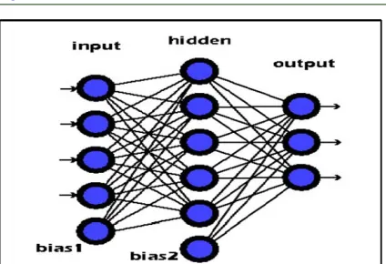
A Multi-Layer Neural Network (MLP) consists of a number of neurons layers as shown in figure (1). The first layer represents the inputs signals to the neural network, the second layer is the hidden layers that confirm the non-linearly of the model and the last layer that contains the outputs of the network. In the simplest arrangement, each layer in hidden part is connected with the previous layer and the next layer finally will produce an output vector from the previous layers.

The output of a layer is computed by applying the neuron activation function for all neurons on the layer as in equation:

Y =

f



wx



b



Where w represents a weight assigned to each pair

of neurons from layer input to hidden layer or from

hidden to output layer and b is a vector of bias terms

for each neuron in layers and x is the input from the

previous layer [16].

In a classification task the output neuron uses the Softmax activation function to generate a good probability distributions on the outputs. Equation (1) is applied from the first layer up to the last layer (output layer) in sequence (feed forward).

Figure 1: Three Layers of Neural Network

When train MLP an error function used to show if the network is understanding the data or not. There are two error functions that can be used: the first one is Square Error Function (Equation (2)) and the second function is the Cross-Entropy Error Function (Equation (3)). Those two equations are described the error of a one pattern in the dataset [17].

E =















_

i

i t

i

t

y

2

1

(2)

E =

















i

t

i

y

t

_i

log

Where y is the output in the last layer of the

model and t is the identity of the example in dataset.

The main objective of the training model is to minimize the proportion and minimize the mean of error function applied to all cases in the dataset. This process is completed by using stochastic gradient decent [18]. It works with the derivative of the error function concerning the model parameter of the gradient as in equation:

hj h

h i

i

hj

w

z

z

y

y

E

w

E

















_

(4)

Where yi represents the output of the neuron, zh

represents the output before applying the activation

function, and whj are the weights.

ISSN: 1992-8645 www.jatit.org E-ISSN: 1817-3195

5073 Usually, computing starts from the last layer, first calculating the derivative of the error function with regard to zi:













_



t

Z

E

y





For the derivatives with respect to the weights, we obtain the formula:















_y

i t ij t i

w

Z





For the derivatives with respect to the biases, we obtain the formula:

1



b

Z





For the derivatives with respect to the inputs ﻭ

we obtain the formula:

w

y

Z





The equations (6 and 7) are adequate to calculate the derivatives with respect to the weight and bias of a last layer, and the derivative with respect to the output of the layer L -1. The other equation is the derivative of the activation function of the layers 1 until L − 1. The derivative of sigmoidal function is described below:











 



_y

_y

y

Z

1





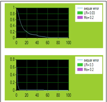
The speed and accuracy of the learning process of updating the weights also depends on a learning rate as shown figure (2).

Figure 2: Factor of Learning Rate and Momentum

Figure (2) show the ability of training with deference parameter of learning rate which is 0.03 and 0.3. When the x-axis represent a number of epochs and y-axis represent an error rate of the learning.

The learning rate specifies how fast the neural network will learn. This is usually a value around one as percent. Another factor of training is the momentum that specifies how much of an effect the previous training iteration will effect on the current iteration. The momentum is also a percent and is usually a value near one [12].

Step 1:

Compute the derivative of errors in the last layer.

Step 2:

Compute the derivative of outputs before computed the activation function.

Step 3:

Compute the derivative of weights wij.

Step 4:

Compute the derivative of bias bj.

Step 5:

5074 3. DEEP BELIEF NETWORKS

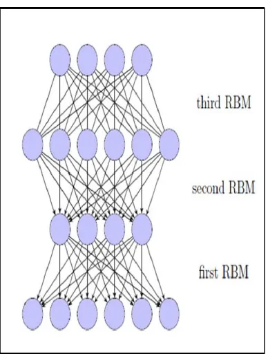
A Deep Belief Networks is a generative learning models that have been introduced by Hinton & Salakhutdinov [19]. They described a DBN as a stacked of restricted Boltzmann machines [19]. DBN aimed to learn structures of the inputs given as a dataset and one or more layers for features detectors.

A DBN is a mix of two representations: directed and undirected graphical models, the top layer of the network is an undirected RBM, and the lower layers are directed as shown in figure (3).The training in deep belief networks is done by one layer at a time. The learning strategy consists of two phases;

 The first is unsupervised learning, which is

called pre-training phase.

 The second phase is a refinement phase,

the network is unfolded as a feed forward neural network in which the weights of hidden units are initialized using the forward weights of the conforming RBMs.

A competitive layer is added as final output layer of the feed forward network, which is trained using a supervised algorithm, to classify the inputs into the appropriate class type [19].

Figure 3: Describe Deep Belief Network

3.1 Restricted Boltzmann Machines

Restricting the connections between nodes in a Boltzmann machine to only those between visible and hidden nodes gives elevation to the Restricted Boltzmann Machine (RBM). Figure (4) describes a simplicity ordering of an RBM within six visible nodes and four hidden nodes.

Figure 4: Restricted Boltzmann Machine

RBMs can themselves be used as regression, classification, or generative models attaching either a single regression label or a SoftMax class label to the visible units that are used for supervised learning and a training models. They can generate a sample of the data distribution that gives a clamped visible label unit. The need of describing a RBM in this study to constructing of a DBN, and training it with an unsupervised learning model [11][12][16].

3.2 Training a Restricted Boltzmann Machine Training of an RBM keeps track of the same basics in any case of its purposed use. The energy function used as a particular state of stochastic binary visible and hidden units is:

(10)

Where θ is the model parameters and the value of a and b are the visible and hidden unit biases, respectively, and the w refers to the weights of networks that connect the two layers.

The restriction of RBM connection layers inherent very simplification of the Gibbs sampling used in learning and generation model. Since the hidden units and visible units factorize completely, Gibbs sampling for the whole hidden or visible layers that can be executed in a parallel way.

ISSN: 1992-8645 www.jatit.org E-ISSN: 1817-3195

5075 (11)

Averaged over the training set, we find the often-seen rule:

(12)

Unfortunately, finding this precisely is

unmanageable, so samples can be gotten by using Gibbs sampling. Sampling takes less time, however achieving an appropriate stationary circulation is frequently still undesirable because of the need to achieve the stationary dispersion of the Markov chain. A breakthrough in speeding up this learning procedure was sketched out by Hinton and named Contrastive Divergence that computing the log-likelihood gradient of RBM specifically is regularly not done straightforwardly because of the parcel capacity, so approximations are utilized. Hinton presented Contrastive Difference (CD) [20] as a technique to get estimated samples without a larger number of Gibbs sampling steps.

Hinton found that augmenting the log-likelihood over the information dissemination is equivalent to minimizing the Kullback-Leibler uniqueness between the information distribution and the balance dispersion of the model after Gibbs sampling.

The general thought behind CD is that even only a few steps of the Markov chain will give a heading to the slope in the state space for the Markov chain, and provide the training algorithm with the suitable redress to the gradient. Running the chain for an infinite number of steps would give us the accurate redress for the model parameters. However, this is clearly recalcitrant too.

Typically, the CD algorithms is running for one full steps of Gibbs sampling. The visible units are

initialized with the training data (v0), h0 is sampled

from p (hj v0), and v1 is sampled from p (vj h1).

Then, the log-likelihood for v0 is approximated by [19][20]:

(13)

Even with this approximation and the variance that it introduces to the learning process, empirical results show that this is an effective and efficient learning algorithm.

4. EXPERIMENTAL SETUP

In this section the experimental setup used for English Character Recognition is described.

4.1. Dataset

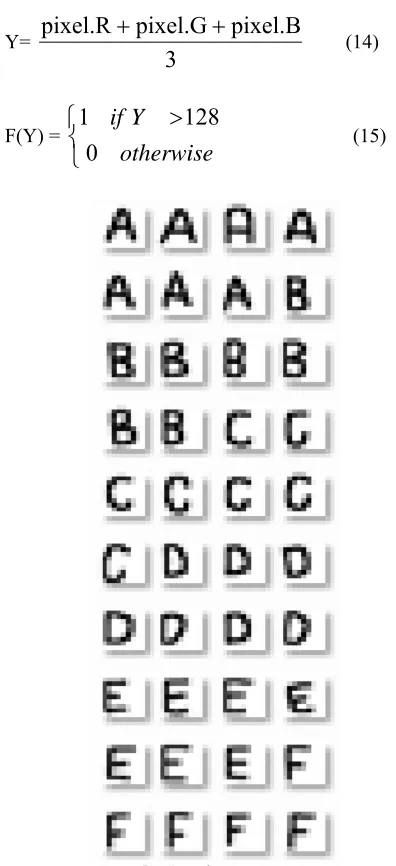
The dataset is composed of 260 images of size 10 by 10 pixels in gray scale which is representing characters (A-Z) at which there are 10 images for each character in different write shape. Some examples are shown in figure (5). The dataset is divided into two parts, one for training that take 70% from dataset (182 images), and others take 30% for testing (78 images). Images have been stochastically binaries according to their pixel intensity as:

Y=

3

pixel.B

pixel.G

pixel.R





(14)

F(Y) =









otherwise

Y

if

0

128

1

(15)

5076 4.2. Methodology

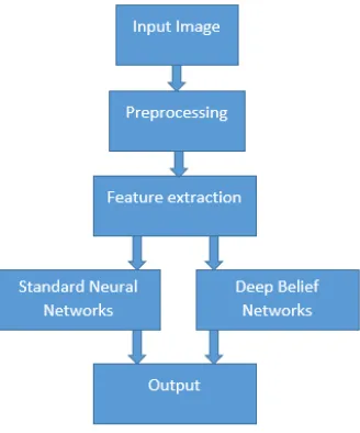
In this section we describe the methodology of the paper which is shown as figure (6).

Figure: (6) Describe the Methodology

The preprocessing stage is to extract the features that the first step take the picture from drawing panel and resize the image to 10 x 10 pixel as shown figure (7).

Figure: (7) Resize Image

After that the resized step the image will convert to white and black depending of the intensity of the pixel. The threshold of convert the image to binary set to 128 and if the value of the pixel greater than threshold then set one otherwise set zero as shown figure (8).

Figure: (8) Binaries Image

After complete the previous step the input will generate by build vector that take row by row of the image to build the final representation of the feature of the character. As shown figure (9).

Figure: (9) Feature Extraction

All samples of dataset take the same processing and the final presentation of the dataset as a 250 rows, each one refer to one sample as shown in figure (10).

Figure: (10) Samples Features

ISSN: 1992-8645 www.jatit.org E-ISSN: 1817-3195

5077

Figure: (11) Neural Network Architecture

The algorithms of BP describe bellow:

Also in the architecture of the Deep Belief Networks in figure (6) we use the same input contain of 100 neurons (image 10 by 10) as an inputs layer that represent as vector of zero and one and hidden layer within variable number (v) that change in each training network to produce the best Deep Belief Network. In the end of networks the 26 neurons represented as an output layer (26 Characters).

Each neuron in output layer represent as a class of character depend on the index of these character as shown figure (12).

Figure: (12) Deep Belief Network Architecture

The parameter input, hidden and output layers as the same as Standard Neural Networks parameter for comparing purpose between them. But the training be in two phases the first phase adjusting the weight between the input and hidden neurons by unsupervised learning using contrastive divergence algorithm. And the second phase by supervised learning using the backpropagation algorithm. The training in Deep Belief Network learn each layer at one time.

The learning will work in the first phase as unsupervised using CD algorithms and adjust the weight for all epoch then move to the next phase as

supervised learning using backpropagation

algorithms.

The algorithms of CD describe bellow: Algorithm 1: Backpropagation (BP)

Input: Training inputs, training outputs.

Output: Best weights.

Goal: Optimize the weights to make the neural network correctly mapping arbitrary inputs to outputs.

Forward:

Step1: for all layers in the network:

 Compute the summation multiple weight.

 Compute the output by activation function  Backward:

Step2: For the outputs of step1:

 Compute the derivative for the output.

 Compute the output gradient depend on the derivative.

Step3: For the hidden layer:

 Compute the derivative for hidden layer.

 Compute the hidden gradient depend on the derivative.

Step4: For the inputs by hidden neurons:

 Compute the delta as multiply learning rate by gradient.

 Update weights between inputs and hidden.

Step5: For the hidden by output neurons:

 Compute the delta as multiply learning rate by gradient.

5078 5. RESULTS

Tests were run on a laptop computer with Intel® Core i3 CPU 2.40 GHz processor, 4GB of RAM. Firstly we do an experiment with large iteration numbers saying 1000 training epochs to have a general sense about error rate. Figure (13) shows mean square error for training phase with 1000 iterations.

Figure 13: Mean Square Error for 1000 Iteration

The feed forward neural networks are evaluated based on backpropagation learning algorithm. Here the class labels were used based on value in the nodes at the output layer. While Deep Belief Networks was pre-trained using unsupervised learning contrastive divergence. The pre-trained weights were used as the initialization for the feed forward neural networks. The weights are fine-tuned using Error Back-propagation learning algorithm.

The experiment for the number of hidden layer is a six experiment that the first is 50 neuron that training as a 200 epoch it take about 1:17 min/sec in a standard neural networks give an accuracy of 85.8% while the same parameter in deep belief network take about 1.27 min/sec give an accuracy of

92.3%. These result show the deep belief network take more time but it take a high accuracy comparing to standard neural networks. The Result of two models are shown in table (1) that show the result of ANN and table (2) show the result of DBN.

Table 1:.Results of Standard Neural Network.

Architecture

Neural networks

T F Error _Rate Time _train Time _test

100-50-26 67 11 14.102 1:17.18 0.09

100-80-26 68 10 12.82 1:52.41 0.106

100-100-26 65 13 16.666 2:20.93 0.113

100-120-26 67 11 14.102 2:41.37 0.120

100-150-26 65 13 16.666 3:20.39 0.147

100-200-26 66 12 15.384 4:19.29 1.695

Table (1) show the accuracy of neural networks with different architecture of networks. It show that the best architecture when the number of hidden layer is 80 neurons. The networks test on the 78 samples and gives an 87.12% with 10 misclassified samples. The training of this architecture take about two hour for training and 0.1 second for testing all samples.

Table 2:.Results of Deep Belief Network.

Architecture

Deep belief network T F Error _Rate Time _train Time _test

100-50-26 72 6 7.6923 1:27.45 0.04

100-80-26 69 9 11.538 2:05.44 0.04

100-100-26 71 7 8.9743 2:31.95 0.04

100-120-26 69 9 11.5384 2:56.21 0.053

100-150-26 69 9 11.5384 3:37.51 0.054

100-200-26 69 9 11.5384 4:40.35 0.065

Table (2) show the accuracy of Deep Belief Networks with different architecture of networks. It show that the best architecture when the number of hidden layer is 50 neurons. The networks test on the 78 samples and gives a 92.3% with only 6 misclassified samples. The training of this architecture take about 90 minutes for training and 0.04 second for testing all samples.

The recognition accuracy is calculated as the ratio of the sum of all character with correct recognition to the entire set of character in the training set. The best accuracy success is 92.3% with deep belief network with one RBM.

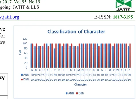
For each character in dataset, we also calculate its classification rate as table (3). It shows in ANN that some characters have identifying rate as high as 90% to 100% but the worst case character G can just Algorithm 2: Contrastive Divergence (CD

Input: RBM visible and training data.

Output: Best weights of RBM.

Step1: Initialize weights by using Gaussian function with Alf =0.1.

Step2: For all samples in the training set:

 Apply the sample to the RBM.

 Compute the probability of hidden layer.

 Compute the probability of visible layer.

Step3: For each visible and hidden:

 Compute the gradient.

Step3: For each input by hidden weights:

ISSN: 1992-8645 www.jatit.org E-ISSN: 1817-3195

5079 achieve 80%. While in DBN the character have identifying rate as 90% to 100% for all test for training and testing data and figure (14) shows visual comparing between two algorithms.

Table 3:.Results of Deep Belief Network.

  NO. Of  Classified 

in ANN 

NO. Of  Classified 

in DBN 

Accuracy Accuracy

A  10  10  100 %  100%

B  9  10  90 %  100%

C  9  9  90 %  90%

D  9  10  90 %  100%

E  10  9  100 %  90%

F  10  10  100 %  100%

G  8  10  80 %  100%

H  10  10  100 %  100%

I  9  10  90 %  100%

J  10  10  100 %  100%

K  9  10  90 %  100%

L  9  9  90 %  90%

M  9  10  90 %  100%

N  10  10  100 %  100%

O  10  10  100 %  100%

P  10  10  100 %  100%

Q  10  10  100 %  100%

R  10  9  100 %  90%

S  10  10  100 %  100%

T  10  10  100 %  100%

U  10  10  100 %  100%

V  9  10  90 %  100%

W  10  10  100 %  100%

X  10  10  100 %  100%

Y  10  10  100 %  100%

Z  9  10  90 %  100%  

The average accuracy recognition rate for all data training and testing in ANN give 95.7% while in DBN the accuracy is 98.4%.

Figure 14: Describe Successful Rate For Each Character

6. Conclusion and Future work

A comparing of Neural Networks and Deep Belief Networks for Character Recognition is described to identify 26 uppercase. Multilayer Perceptron’s are initialized with random weights whereas DBNs are initialized with Gaussian weights that trained using unsupervised Contrastive Divergence Procedure. The parameter of BP is very important for training phase that the number of hidden neuron referring to higher factor in both algorithms and learning rate is another important factor. DBN is a faster than NN in training and testing it train and accepted the information speediest of NN. DBNs gave a higher performance as compared with the NN with an accuracy of approximately 92.3% for Character Recognition.

The future work is to improve deep learning algorithms using another classification algorithms such as spiking neural network instead of BP with DBN and show the effected of the classification.

REFRENCES:

[1] Ethem Alpaydın,” Introduction to Machine

Learning”, Third Edition, the MIT Press Cambridge, Massachusetts London, England, 2014.

[2] Cory Lesmeister, “Mastering machine learning

with r”, 2015.

[3] Li Deng, Dong Yu, “Deep Learning Methods

and Applications”, Foundations and Trends® in Signal Processing Volume 7 Issues 3-4, ISSN: 1932-8346, 2014.

[4] Kyunghyun Cho, “Foundations and Advances

in Deep Learning”, 2014.

[5] Yann LeCun, Yoshua Bengio , Geoffrey

Hinton, “Deep learning”,

DOI:10.1038/nature14539, 2015.

[6] Geoffrey E. Hinton, Simon Osindero (2006) 'A

5080

[7] Yoshua Bengio, Pascal Lamblin, Dan Popovici

and Hugo Larochelle (2006) Greedy Layer-Wise Training of Deep Networks, Departement dInformatique et Recherche Operationnelle.

[8] Dan Ciresan, Ueli Meier, Jonathan Masci and

Jurgen Schmidhuber (2012) 'Multi-Column Deep Neural Network for Trafic Sign Classication', Neural Networks.

[9] Dumitru Erhan, Aaron Courville, and Yoshua

Bengio (2010) Understanding Representations Learned in Deep Architectures, Departement dInformatique et Recherche Operationnelle.

[10]Olaf Booij, “Temporal Pattern Classification

using Spiking Neural Networks”, Universiteit van Amsterdam (2004).

[11]Subha Manoharan, “Gaussian Discrete

Restricted Boltzmann Machine theory and its application“, Massey University NewZlanda (2015).

[12]Gilberto Batres-Estrada, “Deep Learning for

Multivariate Financial Time Series”, (2015).

[13]Simon Haykin, “Neural Networks and Learning

Machines”, 3rd edit., McMaster University Hamilton, Ontario, Canada (2009).

[14]DONALD L. EPLEY, “Reviews of Books and

Papers in the Computer Field”, IEEE TRANSACTIONS ON COMPUTERS, (1969).

[15]KURT HORNIK “Multilayer Feedforward

Networks are Universal Approximators”, Neural Networks, pp. 359-366, (1989).

[16]LUIZ GUSTAVO HAFEMANN, “AN

ANALYSIS OF DEEP NEURAL

NETWORKS FOR TEXTURE

CLASSIFICATION”, CURITIBA University, (2014).

[17]Pavel Golik, Patrick Doetsch, Hermann Ney,

“Cross-Entropy vs. Squared Error Training: a Theoretical and Experimental Comparison”, RWTH Aachen University, (2014).

[18]Pedro Paulo Marques do Nascimento

“APPLICATIONS OF DEEP LEARNING TECHNIQUES ON NILM”, Rio de Janeiro, (2016).

[19]Ruslan Salakhutdinov, Andriy Mnih, Geofirey

Hinton, “Restricted Boltzmann Machines for Collaborative Filtering”, University of Toronto, (2006).

[20]Geoffrey E. Hinton, “Training Products of

Experts by Minimizing Contrastive