Two New Iterated Maps for Numerical Nth Root Evaluation

(1)

http://dx.doi.org/10.4236/am.2014.519283

How to cite this paper: Dias, C.C., Dellajustina, F.J. and Martins, L.C. (2014) Two New Iterated Maps for Numerical Nth Root Evaluation. Applied Mathematics, 5, 2974-2981. http://dx.doi.org/10.4236/am.2014.519283

Two New Iterated Maps for Numerical Nth

Root Evaluation

Charles Corrêa Dias

1

_{, Fernanda Jaiara Dellajustina}

2

_{, Luciano Camargo Martins}

2* 1_{Department of Electrical Engineering, Universidade do Estado de Santa Catarina (UDESC), Joinville, Brazil} 2_{Department of Physics, Universidade do Estado de Santa Catarina (UDESC), Joinville, Brazil}

Email: [email protected], [email protected], *_{[email protected]}

Received 15 August 2014; revised 10 September 2014; accepted 6 October 2014

This work is licensed under the Creative Commons Attribution International License (CC BY).

http://creativecommons.org/licenses/by/4.0/

Abstract

In this paper we propose two original iterated maps to numerically approximate the nth root of a real number. Comparisons between the new maps and the famous Newton-Raphson method are carried out, including fixed point determination, stability analysis and measure of the mean con-vergence time, which is confirmed by our analytical concon-vergence time model. Stability of solutions is confirmed by measuring the Lyapunov exponent over the parameter space of each map. A gene-ralization of the second map is proposed, giving rise to a family of new maps to address the same problem. This work is developed within the language of discrete dynamical systems.

Keywords

Iterated Map, Nth Root of a Real Number, Numerical Method, Newton-Raphson Method, Dynamical System

1. Introduction

Recent applications of iterated maps in numerical analysis have been found in literature, using and extending the techniques of dynamical systems to the study of numerical algorithms and number theory [1]-[3]. Application in technology and hardware devices are also frequent nowadays [4]-[7].

We propose and study in this work two new methods for numerical root approximations, both of which based on iterated maps. In the following sections we present a detailed study of each map, their fixed points and stabil-ity, the occurrence of bifurcations and chaotic behavior.

(2)

WAM.

2. The First Dias Map (FDM)

The map which we will study now was created by Charles C. Dias to extract real roots of numbers numbers, by solving the equation xn =k. The proposed map is one-dimensional and is defined as

1 1

1

. 2

i i n

i k x x x + −   =  + 

  (1.1)

Comparing this with the Newton-Raphson Method (NRM) equation and Babylonian Method (BABM) [10] noticed that this statement is a mixture of both, and the FDM is an arithmetic average between the linear and nonlinear terms in Equation (1.1), and can be used to approximate the nth root of k>0 for n∈

( )

0, 4 , as we shall see. Outside this interval of n, this map presents chaotic dynamics through after entering a bifurcation cascade, whose roots having no longer relationship to the nth root of k.

The base function that appears in the iterated map defined by Equation (1.1) can be derived dividing n

x =k

by n1

x − , for x≠0, leading to

1,

n

k x

x−

= (1.2)

and adding x at both sides, and dividing it by 2, we recover functional form of Equation (1.1).

2.1. Geometrical Construction

To construct geometrically the FDM time series, the first step is to find the auxiliary equations of the lines A B_i

(see Figure 1), writing their slopes m_i = ∆ ∆y_i x_i . From this figure, ∆ =y_i f x

( )

_i +k and ∆ =x_i x_i, and the slopes

( )

, 0,1, 2, 3,

i i

i

f x k

m i

x

+

= =  (1.3)

that for f x

( )

=xn−k are n 1

i i

m =x− .

Knowing that their linear coefficients are all −k, then all the auxiliary lines pass through the point B

(

0,−k

)

, we obtain the working lines y x

( )

=x_in−1x−k and the auxiliary points s_i, the intersections points of the work-ing lines with the X-axis, are

1, 0,1, 2, 3, ,

i n i

k

s i

x −

= =  (1.4)

and taking the arithmetic mean between the auxiliary points s_i and the x_i points we recover the original FDM equation (Equation (1.1)).

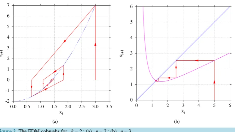
Figure 2(a) shows the cobweb for the FDM time series for n=2 and k=2, and Table 1 (top) shows time

(3)

[image:3.595.206.428.87.237.2]

Figure 1. The FDM schematic geometrical path construction.

(a) (b)

Figure 2. The FDM cobwebs for k=2: (a) n=2; (b) n=3.

shows a numerical development of the FDM series for the parameters n=3 and k=2, based on the time se-ries shown in Table 1 (bottom), where the convergence to the root occurs after 27 steps. Some intermediary time steps are omitted in this table.

2.2. Fixed Point and Stability Analysis

Solving f x

( )

∗ =x∗ we find the FDM fixed point to be n

x∗= k. Applying the stability criterion [11], to the map function f x

( )

=

(

x+k xn−1

)

2, whose derivative is f′

( )

x = −

(

1 k n

(

−1

)

xn

)

2 we obtain 1−n 2 <1, and solving the last equation we have the range of parameter n∈

[ ]

0, 4 where the fixed point of the map is sta-ble.

2.3. Numerical Results

The FDM time series have different dynamics depending on the parameters

( )

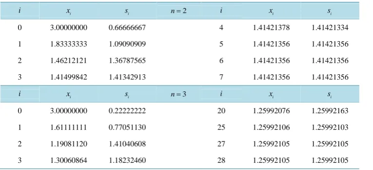
k n, , presenting a fixed point, pe-riodicity or chaos, as occurs to the logistic map [12].

[image:3.595.117.513.263.485.2]

(4)

1 1.61111111 0.77051130 25 1.25992106 1.25992103

2 1.19081120 1.41040608 27 1.25992105 1.25992105

3 1.30060864 1.18232460 28 1.25992105 1.25992105

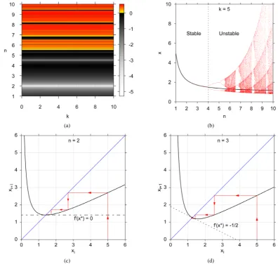
goes to zero signing the period bifurcations. The yellow to red regions indicate the a positive Lyapunov expo-nents, the signature of chaos.

The FDM bifurcation diagram, discarded a transient of 103 iterations and plotted the next 500 values of x, is depicted in Figure 3(b). The values of n studied are uniformly distributed in a grid of 600 points in the interval

[

1,10 . Also plotted over the bifurcation diagram is the exact root

]

nk, the fixed point of the map, plotted in black.

We also study numerically the FDM return diagrams for different values of the parameter n, for k=2 and

0 5

x = , as seen in Figure 3(c) and Figure 3(d), respectively.

3. The Weighted Average Map (WAM)

Instead of adding x, if a more general term px is added in Equation (1.2), we get a new map (WAM) that depends on parameters n, k and p. The new parameter p is a positive real number and corresponds to the weight of the linear term of the map. This term is directly linked to the parameter n, since for each value of n

there is a minimum value of p for the fixed point to be stable, as we shall see. Adding px to both sides of Equation (1.2) we gain

1

n

k px x px

x−

+ = + (1.5)

and after collecting x and dividing by

(

p+1

)

it leads to the new map (WAM),

1 1

,

1 n

k

x px

p x −

 

= _ + _

+   (1.6)

and solving its fixed point equation x_i₊₁ =x_i =x∗ we obtain the expected value n

x∗= k.

3.1. Fixed Point and Stability Analysis

Applying the stability criterion [11], i.e., f′

( )

x∗ <1, to the map function

( ) (

1 1

)

(

n1

)

f x = p+ px+k x −

whose derivative is f′

( )

x =

(

p k n−

(

−1

)

xn

)

(

p+1

)

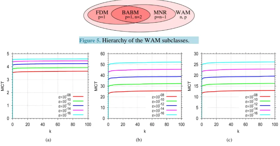
and solving this inequality we obtain p>n 2 1− to guarantee fixed point stability, and Figure 4 shows the line corresponding to this condition, below which the fixed point is unstable. As n is increased the value of p should also be increased to avoid the unstable region, where the time series do not converges to the fixed point.

3.2. WAM Subclasses and Hierarchy

A special subclass of WAM is FDM, when p=1, so that the fixed point on the map according to Figure 4, is sta-ble in the range [1, 4] for n, thus in accordance with the stability analysis the fixed point n

[image:4.595.113.496.101.276.2]

(5)

.

(a) (b)

[image:5.595.114.511.87.463.2]

(c) (d)

Figure 3. (a) FDM Lyapunov exponent over the parameter space

( )

k n, ; (b) the bifurcation diagram showing

the stable fixed point for n∈

( )

0, 4 ; return diagrams for x₀=5 and k=2: (c) n=2; (d) n=3.

(a) (b)

[image:5.595.123.510.505.689.2]

(6)

assumes the value 1−n2 when p=1 (FDM) and is zero only if p= −n 1 (NRM or BABM, if n=2). In

Figure 3(c) we observe that f′

( )

x∗ =0, for n=2 FDM reduces to NRM, and in Figure 3(d), we observe

that f′

( )

x∗ = −1 2.

4. Mean Convergence Time (MCT)

This section reports the numerical results for the mean convergence time (MCT) for NRM, FDM and WAM, based on the average number of iterates to converge within different precisions

ε

, from single

( )

10−8 to double

(

10−16

)

. For this, we varied k on a uniform grid with 103 points in the interval [10−1,102], varying the initial condition x₀ on a second uniform grid with 103 points, whose limits are given by a maximum relative difference of 25% around the exact value of the root of k at each point. Using this schema, the MCT is computed for cubic roots

(

n=3

)

, and for WAM we set p=3. Figures 6(a)-(c) show the numerical results.

In Figure 6(a) we see that the NRM MCT is close to 4, which means that after 4 iterations, on average, there

has been convergence to the root. From this figure, we conclude that FDM is around 10 times slower than NRM, and WAM is around has twice the speed of FDM. In this test, the most efficient is NRM, with the lowest MCT.

Both NRM and FDM belong to the same WAM family, as discussed in Section 3, and the stability of the fixed point n

[image:6.595.90.539.455.690.2]

k of WAM depends on the parameters n and p. Changing the parameter p of WAM we get a new map subclass, for example, for n=2 have the FDM. From these fact, we tried to detect numerically the

Figure 5.Hierarchy of the WAM subclasses.

(a) (b) (c)

Figure 6. Numerical results of MCT for cubic roots

(

n=3

)

calculation with different precisions ε from ₁₀−8

to ₁₀−16

(7)

optimal value of the parameter p, to minimize the ACT over the whole WAM family. For this we used a FORTRAN program to measure extensively the WAM MCT varying parameters

(

n p,

)

on a uniform grid of 500 500× points, for a radicand k. The result for k=2 is shown in Figure 4(a). The region in gray corresponds to unstable fixed point n

k map WAM, as found in Section 1.3. The other colors seen in the graph are the regions of stability of the fixed point. For best visualization the MCT scale of this figure is truncated at a maximum value of 20, and higher values as inked light gray.

We can see in Figure 4(a) that, as we approach the line that corresponds to the weighting term, NRM shows the minimum MCT over this line and therefore the most efficient of all studied maps is the NRM.

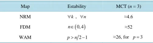
Summarizing the key information about NRM, FDM and WAM, with the numerical results for the MCT within double precision for these maps, for the parameters n=3 and k∈ 10 ,10−1 2_, as shown in Table 2.

Analytical Convergence Time Model

The Lyapunov characteristic exponent for a unidimensional map x_i₊₁= f x

( )

_i usually defined by

( )

( 1)

_{( )}

0 0

1

lim_N _iN ln _i

x f x

N

λ −

→∞ = ′

=

∑

can be approximate by λ∗≈ln f′

( )

x∗ since the derivative of the mapping function at the fixed point f′

( )

x∗

defines the rate of convergence of its time series, after discarded the transient.

For WAM, it is easy to show that f′

( )

x∗ = −1 n

(

p+1

)

, so that this derivative assumes the value 1−n2 when p=1 (FDM) and is zero only if p= −n 1 (NRM or BABM, if n=2). In Figure 3(c)we observe that

( )

0

f′ x∗ = , for n=2 FDM reduces to NRM, and in Figure 3(d), f′

( )

x∗ = −1 2.

Using the original Lyapunov’s idea, the characteristic exponent λ measures the average rate of convergence between two solutions separated by an initial distance ε₀, that is the case of time series dominated by a fixed point. For this orbits, the distance after i iterates is ₀ei

i λ

ε =ε so that, if we assume that one orbit is initialized at x₀ =x∗ and other at x₀=x∗+1, i.e., the initial distance is unitary between orbits, we can use last equation to measure the error found in the second orbit, the root to be approximated. Within the standard double precision, the maximum error is of order 10−D, where D is the number of decimal significants, typically D=15 16∼ places.

Applying the natural logarithm to both sides of the above equation we have i ln

( )

εi

λ

= for the number of

iterations needed to reduces the error in the second orbit to

ε

. In the same manner we defined MCT, we define now the analytical convergence time (ACT), estimated by

( )

ln10 , ln D ACT

f x∗

− ≈

′ (1.7)

valid for any fixed point of a unidimensional map, where the approximated λ∗ was used. Applying this model to our more general map (WAM), we have

(

)

ln10

₍

₎

,

ln 1 1

D ACT n p

n p

− ≈

− + (1.8)

[image:7.595.171.423.647.718.2]

of the parameters n and p. To double precision this approximated model function is plotted in Figure 4(b), that is remarkably very close to the numerical version plotted in Figure 4(a). Both figures uses the same color palette and truncated maximum, for better comparisons.

Table 2. MCT numerical results for NRM, FDM and WAM maps.

Map Estability MCT (n = 3)

NRM ∀k, ∀n ≈4.6

FDM n∈

( )

0, 4 ≈52

(8)

general class of map studied. The model presented in Equation 1.7 is general, and can be adapted to any unidimensional map to study its fixed point attractor.

The main results of this work are obtained for x∈, but their generalization is straightforward over the complex set .

Acknowledgements

This work was partially supported by the Brazilian agency Conselho Nacional de Desenvolvimento Cientfico e Tecnológico―CNPq and Universidade do Estado de Santa Catarina―UDESC.

References

[1] Faber, X. and Voloch,J.F. (2011) On the Number of Places of Convergence for Newton’s Method over Number Fields. Journal de Theorie des Nombres de Bordeaux, 23, 387-401.

[2] Grau-Sánchez, M. and Daz-Barrero, J.L. (2011) A Technique to Composite a Modified Newton’s Method for Solving Nonlinear Equations. ArXiv e-prints.

[3] Pan, B., Cheng, P. and Xu, B. (2005) In-Plane Displacements Measurement by Gradient-Based Digital Image Correla-tion.SPIE Proceedings, 5852, 544-551.

[4] Amin, A.M., Thakur, R., Madren, S., Chuang, H.-S., Thottethodi, M., Vijaykumar, T., Wereley, S.T. and Jacobson, S.C. (2013) Software-Programmable Continuous-Flow Multi-Purpose Lab-on-a-Chip. Microfluidics and Nanofluidics, 15, 647-659. http://dx.doi.org/10.1007/s10404-013-1180-2

[5] Mungan, C.E. and Lipscombe, T.C. (2012) Babylonian Resistor Networks. European Journal of Physics, 33, 531.

http://dx.doi.org/10.1088/0143-0807/33/3/531

[6] Senthilpari, C., Mohamad, Z.I. and Kavitha, S. (2011) Proposed Low Power, High Speed Adder-Based 65-nm Square Root Circuit. Microelectronics Journal, 42, 445-451. http://dx.doi.org/10.1016/j.mejo.2010.10.015

[7] Sun, T., Tsuda, S., Zauner, K.-P. and Morgan, H. (2010) On-Chip Electrical Impedance Tomography for Imaging Bio-logical Cells. Biosensors and Bioelectronics, 25, 1109-1115. http://dx.doi.org/10.1016/j.bios.2009.09.036

[8] Ausloos, M. and Dirickx, M. (2005) The Logistic Map and the Route to Chaos: From the Beginnings to Modern Ap-plications. Springer, New York.

[9] Eve, J. (1963) Starting Approximations for the Iterative Calculation of Square Roots. The Computer Journal, 6, 274- 276. http://dx.doi.org/10.1093/comjnl/6.3.274

[10] Dellajustina, F.J. and Martins, L.C. (2014) The Hidden Geometry of the Babylonian Square Root Method. Accepted by Applied Mathematics, August.

[11] Lyapunov, A.M. (1992) The General Problem of the Stability of Motion. International Journal of Control, 55, 531- 534. http://dx.doi.org/10.1080/00207179208934253

[12] Schuster, H.G. and Just, W. (2005) Deterministic Chaos: An Introduction. 4th Edition, John Wiley & Sons, New York.

(9)