A Comparative Study of Hill Climbing Based Peak Power Point Tracking Techniques

© 2016, IRJET | Impact Factor value: 4.45 | ISO 9001:2008 Certified Journal

| Page 466

A Comparative Study of Hill-Climbing Based Peak Power Point

Tracking Techniques

Vibhu Jately

_{, Sudha Arora}

1

_{Ph.D. Scholar, Dept. of Electrical Engineering, GBPUA&T, Uttarakhand, India}

_{Professor & Head, Dept. of Electrical Engineering, GBPUA&T, Uttarakhand, India}

---***---Abstract -

important role in photovoltaic (PV) power systems because they extract maxim power output from a PV system for a given set of conditions. The power-voltage characteristic of photovoltaic array is non-linear and generally there exists a single point at which maximum power is available for a specific environmental condition. As the environmental conditions fluctuate throughout the day, maximum power point tracker along with the power converter forces the PV panel to deliver maximum power to the load. Researchers have proposed different techniques to achieve fast and accurate tracking of the maximum power point. Among these techniques, hill-climbing based algorithms are widely used for commercial and industrial applications. In this paper, a comparative performance analysis of the conventional hill-climbing MPPT algorithms is done. In particular, this study compares the behaviours of each technique in presence of solar irradiation variations.

Key Words: mppt, perturb and observe, incremental conductance, incremental resistance.

1.INTRODUCTION

Due to the growing demand on electricity, the limited stock and rising prices of conventional sources (such as coal and petroleum, etc.), photovoltaic (PV) energy becomes a promising alternative as it is omnipresent, freely available, environment friendly, and has less operational and maintenance costs [1]. Therefore, the demand of PV generation systems seems to be increased for both standalone and grid-connected modes of PV systems. Therefore, an efficient maximum power point tracking (MPPT) technique is necessary that is expected to track the MPP at all environmental conditions and then force the PV system to operate at that MPP point. MPPT is an essential component of PV systems. Several MPPT techniques together with their implementation are reported in the literature [2]– [4]. Researchers always feel confused while selecting an MPPT technique for a particular application. Unfortunately, only a few techniques were available in this field including Curve fitting, Fractional Short Circuit Current, Fractional Open Circuit Voltage, Look Up Table, One Cycle Control, Perturb and Observe, Incremental Conductance and Feedback techniques earlier that includes discussions on

MPPT techniques [5]-[8] until 2007. But many new MPPT techniques such as Fuzzy logic, Artificial Neural Network, Adaptive Perturbation and Observation, Estimated perturb and perturb, Genetic Algorithm, Adaptive Neuro fuzzy and particle swarm optimization based MPPT, etc., have been reported since then illustrated in other papers [2]- [4], [11]. Among all the MPPT methods, Perturb & Observe (P&O) and Incremental Conductance (IC) are most commonly used because of their simple implementation and lesser time to track the maximum power point and also other economic reasons. Under suddenly changing weather conditions (irradiation level) as MPP changes continuously, P&O takes it as a change in MPP due to perturbation rather than that of irradiation and sometimes ends up in calculating wrong MPP [9]. However, this problem is eliminated in Incremental Conductance method as the algorithm takes two samples of voltage and current to compute MPP [10]. However, instead of more efficiency the complexity of the algorithm is very high compared to the former one and hence the cost of execution increases. So, we have to extenuate with a trade-off between ramification and efficiency. This paper attempts to provide a comparative review on most of the reported MPPT techniques excluding any unintentionally omitted papers because of space limitations.

2. MATHEMATICAL MODELING OF PV CELL

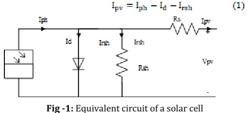
A single diode equivalent circuit shown in Fig. 1 was used to develop the mathematical model of solar cell. The Ipv-Vpv characteristics of this model can be formulated by applying Kirchhoff’s current law (KCL), which is given governed by the following equation:

Fig -1: Equivalent circuit of a solar cell

© 2016, IRJET | Impact Factor value: 4.45 | ISO 9001:2008 Certified Journal

| Page 467

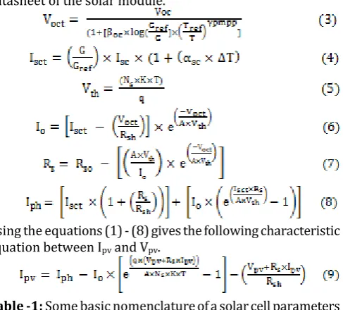
accuracy and the number of parameters in solving the differential equation. A model to calculate the maximum power has been developed by [12]–[14]. The equations used to model the solar panel is given below:

The five parameters Voct, Isct, Vth, Io and Rs are calculated for a given irradiance and temperature from the manufacturers

datasheet of the solar module.

Using the equations (1) - (8) gives the following characteristic

equation between Ipv and Vpv.

Table -1: Some basic nomenclature of a solar cell parameters

Ipv = current of PV cell Vpv = voltage across PV cell Isc = short circuit current of PV cell at

stc Voc = open circuit voltage of the PV cell at stc Impp = current at maximum power of

the cell Vmpp = voltage at maximum power of the cell Pmpp = maximum power of the PV cell Gref = irradiance at standard test conditions

(stc)

G = incident irradiance Gref = irradiance at stc T = temperature of PV cell Tref = temperature of PV cell stc

Isct = short circuit current of PV cell at

given G & T Vgiven G & T oct = open circuit voltage of the PV cell at Irsh = current throught the shunt

resistance

Io = reverse saturation current of diode

Id = diode current Iph = photo current proportional to irradiance G

Rso = series resistance where Vpv is

equal to Voc RIsc sho = shunt resistance where Ipv is equal to Rsh = shunt resistance of the PV cell Rs = series resistance of the PV cell αsc = temperature coefficient of short

circuit current

βoc = temperature coefficient of open circuit voltage.

γpmpp = temperature coefficient of

maximum power Pmpp q = electron charge K = Boltzmann constant A = diode ideality factor

By applying Newton Raphson method to solve (9), the I-V and P-V curve of a 49W Samsung solar module obtained under varying irradiance (1kw/m2_{, 0.8kw/m}2_{, 0.6 kw/m}2_{, 0.4} kw/m2_{) is shown in Fig. 2 and Fig. 3, respectively.}

Fig -2: I-V characteristics of a 49W PV module

As evident from the characteristic graph there is a single operating point in each curve at which the maximum amount of power can be extracted from the solar panel. The mppt algorithm tracks this point and forces the PV module to operate at the voltage (Vmpp) or current (Impp) so that maximum amount of power can be transferred to the load.

Fig -3: P-V characteristics of a 49W PV module

3. MPPT ALGORITHMS

The solar energy conversion efficiency of a photovoltaic cell is around 20-21%. For maximum utilization of the energy under varying atmospheric conditions mppt trackers are employed in most PV applications. Some commonly used mppt techniques are discussed below:

3.1 Perturb and Observe (P&O) Algorithm

Perturbation and Observation (P&O) is an iterative method to track the MPP. Its operation is based on periodic measures of the voltage and current of the PV system to calculate the system power; this value is compared with previous power values and, using this information, the operating voltage of the system is modified (perturbed). If the PV array power is increased (dP/dV > 0), the control system adjusts the PV array operating point in that direction, otherwise, the operating point is moved in the opposite direction. This process is continuously repeated until the MPP is reached; the system keeps oscillating around this point.

© 2016, IRJET | Impact Factor value: 4.45 | ISO 9001:2008 Certified Journal

| Page 468

advantage of this technique is its simplicity, furthermore, previous knowledge of the PV panel characteristics is not required. Two disadvantages of the P&O method are the oscillations around of the MPP and failures due to abrupt changes in weather conditions. The flowchart the P&O method is shown in Fig. 4.

MEASURE V(t) and I(t)

P(t) = V(t)*I(t) dV = V(t) – V(t-1) dP = P(t) - P(t-1) ΔV = PERURBATION STEP SIZE

dP > 0

dV > 0

V(t+1) = V(t) – ΔV V(t+1) = V(t) + ΔV V(t+1) = V(t) – ΔV V(t+1) = V(t) + ΔV

Return

Yes No

No

Yes Yes

dV > 0 No

Fig -4: Flowchart of Perturb and Observe

3.2 Incremental Conductance (INC) Algorithm

The Incremental Conductance method is based on the fact that the slope of the P-V curve of a PV system is zero when the MPP is reached, positive on the left of the MPP and negative on the right:

dP/dV=(d(I.V))/dV= I+V dI/dV (10) To achieve maximum power, the power derivative must be zero.

dP/dV=0 or dI/dV= -I/V, at MPP (11) dI/dV > -I/V, left of MPP

dI/dV < -I/V, left of MPP

where I/V represents the conductance and dI/dV represents the incremental conductance. A disadvantage of the INC method is that if the step size is small, the response of the system to get to MPP is slow. The INC algorithm exhibits less oscillatory behavior around the MPP compared to the P&0 method. The flowchart of this method is shown in Fig. 5. Hence, by comparing the conductance I/V with the incremental conductance dI/dV the algorithm can track MPP.

3.3 Incremental Resistance (INRES) Algorithm

The incremental resistance method is a current analogy of incremental conductance method. The INR differs from INC from the fact that it uses the knowledge of PV power curve (P-I). By examining the P-I curve from Fig. 2 we can easily see that the slope of the power curve is positive on the left side, negative on the right and zero at the peak power point. Thus the algorithm can be developed as follows:

MEASURE V(t) and I(t)

dI = I(t) – I(t-1) dV = V(t) – V(t-1) ΔV = PERTURBATION STEP SIZE

dV = 0

dI/dV = - I/V

V(t+1) = V(t) – ΔV V(t+1) = V(t) + ΔV V(t+1) = V(t) – ΔV V(t+1) = V(t) + ΔV

Return

Yes No

No

No

Yes Yes

dI = 0

dI/dV > - I/V dI > 0

No

Yes No

Yes

Fig -5: Flowchart of Incremental Conductance

dP/dI= (d(V.I))/dI= V+I dV/dI

The condition for maximum power can be calculated by equating the power derivative to zero.

dP/dI=0 or dV/dI= -V/I

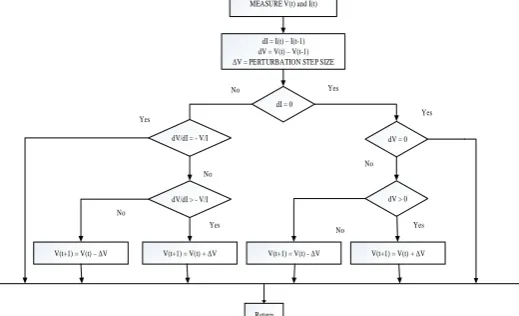
where V/I represent the resistance and dV/dI represents the incremental resistance. The flowchart of the algorithm is shown in Fig. 6.

MEASURE V(t) and I(t)

dI = I(t) – I(t-1) dV = V(t) – V(t-1) ΔV = PERTURBATION STEP SIZE

dI = 0

dV/dI = - V/I

V(t+1) = V(t) – ΔV V(t+1) = V(t) + ΔV V(t+1) = V(t) - ΔV V(t+1) = V(t) + ΔV

Return Yes No

No

No

Yes Yes

dV = 0

dV/dI > - V/I dV > 0

No

Yes No

Yes

Fig -6: Flowchart of Incremental Resistance

4. SIMULATION RESULTS

© 2016, IRJET | Impact Factor value: 4.45 | ISO 9001:2008 Certified Journal

| Page 469

Fig -7: P-t curve showing comparison between P&O, INC and INRES algorithm for an increased step in irradiance

The simulations were carried out for varying irradiance and temperature levels. The simulation result in Fig. 8 shows the output power for a ramp increase/decrease in irradiance. The INRES algorithm displayed excellent dynamic response as compared to P&O and INC algorithm.

Fig -8: P-t curve showing comparison between P&O, INC and INRES algorithm for a ramp increase/decrease in

irradiance

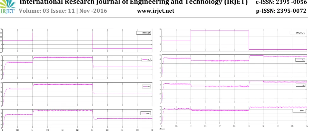
The simulation result for a step increase in temperature is shown in Fig. 9. The results prove that the output power of the INRES algorithm is less affected by temperature variation as it uses P-I curve which is a logarithmic function of temperature. Hence, the output power obtained from P&O and INC algorithm is slightly less than that obtained from INRES algorithm.

The steady state response of the algorithms under STC is shown in Fig. 10. The steady state power oscillations in P&O and INC are much less as compared to INRES algorithm.

Fig -9: P-t curve showing comparison between P&O, INC and INRES algorithm for an increased step in temperature

Fig -10: P-t curve showing steady state comparison between P&O, INC and INRES algorithm under STC

The calculated efficiencies for different irradiance level is presented in Table 2.

Table -2: Efficiencies at different irradiance levels Algorithm Efficiency

(1KW/m2₎

Efficiency

(800W/m2₎

Efficiency

(600W/m2₎

Efficiency

(400W/m2₎

P&O 93.89% 91.32% 88.82% 91.99%

INC 93.69% 91.32% 88.82% 91.99%

INRES 96.34% 90.30% 85.73% 93.55%

5. CONCLUSIONS

© 2016, IRJET | Impact Factor value: 4.45 | ISO 9001:2008 Certified Journal

| Page 470

Incremental conductance performed as well as P&O, but in general its higher implementation cost would not be justified by any improvement in performance.

REFERENCES

[1] M. Ameli, S. Moslehpour, and M. Shamlo,

“Economical load distribution in power networks that include hybrid solar power plants,” Elect. Power Syst. Res., vol. 78, no. 7, pp. 1147–1152, 2008.

[2] A. Dolara, R. Faranda, and S. Leva, “Energy Comparison of Seven MPPT Techniques for PV Systems,” vol. 2009, no. September, pp. 152–162, 2009.

[3] N. Femia, G. Petrone, G. Spagnuolo, and M. Vitelli, Power Electronics and Control Techniques for Maximum Energy Harvesting in Photovoltaic Systems.

[4] V. Salas, E. Olias, A. Barrado, and A. Lazaro, “Review of the maximum power point tracking algorithm for stand-alone photovoltaic system,” Solar Energy Mater. Solar Cells, vol. 90, no. 11, pp. 1555–1578, 2006.

[5] V. Salas, E. Olias, A. Lazaro, and A. Barrado, “New algorithm using only one variable measurement applied to a MPPT,” Solar Energy Mater. Solar Cells, vol. 87, no. 1–4, pp. 675–684, 2005.

[6] J.-A. Jiang, T.-L. Huang, Y.-T. Hsiao, and C.-H. Chen, “Maximum power tracking for photovoltaic power systems,” Tamkang J. Sci. Eng.,vol. 8, no. 2, pp. 147– 153, 2005.

[7] V. Salas, E. Olias, A. Lazaro, and A. Barrado, “Evaluation of a new maximum power point tracker applied to the photovoltaic stand-alone systems,” Solar Energy Mater. Solar Cells, vol. 87, no. 1–4, pp. 807–815, 2005

[8] N. Pongratananukul, “Analysis and Simulation Tools for Solar Array Power Systems,” Ph.D. dissertation,Dept. Electrical and Computer Engineering, Univ. Central Florida, Orlando, FL, 2005.

[9] C. Liu, B.Wu, and R. Cheung, “Advanced algorithm for MPPT control of photovoltaic systems,” in Proc. Canadian Solar Build. Conf., Montreal, QC, Canada, Aug. 20–24, 2004.

[10] S. Jain and V. Agarwal, “A new algorithm for rapid tracking of approximate maximum power point in photovoltaic systems,” IEEE Power Electron. Lett., vol. 2, no. 1, pp. 16–19, Mar. 2004.

[11] Y. Chen, K. Smedley, F. Vacher, and J. Brouwer, “A new maximum power point tracking controller,” in Proc. 18th Annu. IEEE Conf. Appl.Power Electron. Conf. Expo., Florida, 2003.

[12] M. Katsanevakis, “Modelling the Photovoltaic Module,” pp. 1414–1419, 2011.

[13] S. A. Rahman, R. K. Varma, and T. Vanderheide, “Generalised model of a photovoltaic panel,” no. August 2013, 2014.