1
Pruning Methods for Rule Induction
Osama M. Othman
Informatics Research Centre
University of Salford, Salford, UK
2
Contents
CONTENTS... 2
LIST OF FIGURES ... 4
LIST OF TABLES ... 5
ACKNOWLEDGEMENTS ... 6
LIST OF ABBREVIATIONS ... 7
ABSTRACT ... 8
CHAPTER 1: INTRODUCTION ... 9
1.1RESEARCH QUESTION ... 11
1.2MOTIVATION ... 11
1.3CONTRIBUTION TO KNOWLEDGE ... 12
1.4STRUCTURE OF THIS THESIS ... 14
2.1INTRODUCTION ... 17
2.2DEFINITIONS ... 18
2.3AN OVERVIEW OF LEARNING ALGORITHMS ... 19
2.3.1 Instance-Based Learning ... 20
2.3.2 Rule-Induction Algorithms ... 22
2.4AN OVERVIEW OF PRUNING ALGORITHMS ... 28
2.4.1 Instance Pruning ... 28
2.4.2 Rule Induction Pruning ... 34
2.5SUMMARY ... 41
CHAPTER 3: LITERATURE REVIEW: ANT COLONY OPTIMIZATION ... 43
3.1ANT COLONY OPTIMIZATION OVERVIEW ... 43
3.2APPLICATION OF ACO TO CLASSIFICATION RULE INDUCTION ... 49
3.2.1 Ant-Miner Algorithm ... 49
3.2.2 Feature Subset Selection ... 55
3.3SUMMARY ... 59
CHAPTER 4: EXPERIMENTAL FRAMEWORK ... 60
4.1PROBLEM STATEMENT ... 60
4.2BENCHMARK DATASETS ... 62
4.3RULE-INDUCTION CHARACTERISTICS ... 63
4.4ESTIMATING THE PREDICTIVE ACCURACY OF RULES ... 65
4.5COMPARISON EVALUATION ... 66
4.6EXPERIMENTAL SETUP ... 67
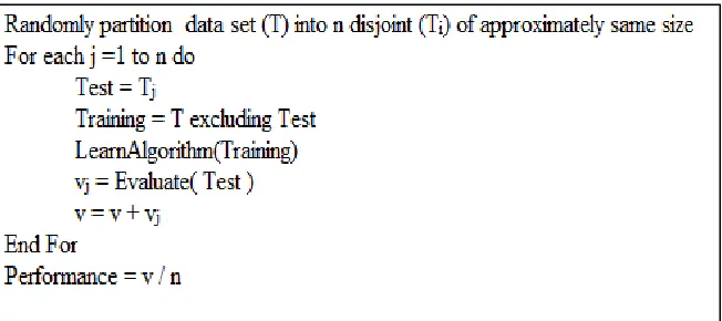
4.6.1 Cross-validation ... 67
4.6.2 Choosing K for K-NN algorithm ... 68
3
4.6.4 Experiment Implementation ... 69
4.6.5 Summary ... 70
CHAPTER 5: PRECEDING RULE INDUCTION WITH INSTANCE-REDUCTION METHODS ... 71
5.1EXPERIMENTATION ... 71
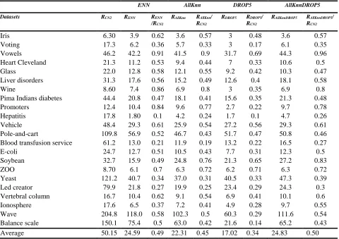
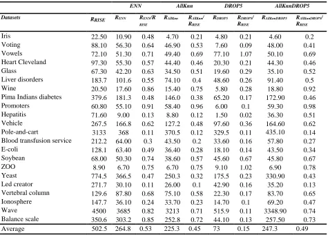
5.2ANALYSIS OF RESULTS ... 72
5.3CONCLUSION ... 81
CHAPTER 6: INSTANCE-REDUCTION METHOD BASED ON ANT COLONY OPTIMIZATION ... 83
6.1ACO-IR ... 84
6.1.1 Initialization of Pheromone Values ... 86
6.1.2 Selecting Subset of Instances (Generation of Solutions) ... 87
6.1.3 Heuristic Function... 88
6.1.4 Fitness Function ... 88
6.1.5 Pheromone Updating ... 89
6.1.6 Number of Ants ... 90
6.2EXPERIMENTAL RESULTS FOR INSTANCE REDUCTION USING THE ACOALGORITHM ... 90
6.3PRUNING CLASSIFICATION RULE USING ACO-IR ... 96
6.4CONCLUSION ... 98
CHAPTER 7: DISCUSSION AND FUTURE WORKS ... 103
7.1THESIS SUMMARY ... 103
7.2MAIN FINDINGS ... 104
7.3FUTURE WORK ... 106
4
List of Figures
Figure 1 Pseudo-code for PRISM algorithm ...27
Figure 2 Pseudo-code for ENN algorithm ...32
Figure 3 Pseudo-code for AllKnn algorithm ...33
Figure 4 Pseudo-code for DROP5 algorithm ...33
Figure 5 A weighted graph for TSP with 5 cities ...46
Figure 6 Pheromone values for the graph in Figure 5 after the first ant finishes a tour ...48
Figure 7 Ant – miner algorithm ...50
Figure 8 Feature subset selection based on ACO ...59
Figure 9 the line or curve separates instances from different classes ...61
Figure 10 Framework for instance-reduction method preceding rule induction ...61
Figure 11 AllKnnDROP5 algorithm ...62
Figure 12 estimating the predictive quality of learning algorithms using cross-validation ...68
Figure 13 comparing the average number of generated rules before and after applying instance-reduction methods for different rule induction ...77
Figure 14 Framework for ACO-IR ...85
Figure 15 ACO-IR algorithm ...86
Figure 16 Comparing elapsed time for ACO-IR with size of training set. ...95
5
List of Tables
6
Acknowledgements
I gratefully acknowledge my PhD supervisor, Dr Chris Bryant, for his continuous encouragement and support during this whole project, from the start of the literature review to the thesis’ conclusion. His advice and expertise in the field of machine learning were crucial to the success of this work. His feedback and explanations also helped me understand how to present ideas and demonstrate the results and analyses.
I would like to thank my local advisor, Dr Khalil el Hindi, for his advice and suggestions in the early stages of this project. Next, I would like to express my sincere thanks to Robin Boswell, who implemented the code for CN2 algorithm in 1990, from which Francisco Reinaldo and Marcus Siqueira created the executable file for Windows XP.
7
List of abbreviations
AI – Artificial Intelligence. ACO – Ant Colony Optimization. IBL – Instance Based Learning. ANN – Artificial Neural Network. NN – Nearest Neighbour.
VDM – Value Difference Metric. FSS – Forward Sequential Selection. BSS – Backward Sequential Selection.
RISE – Rule Induction from Set of Examples. IREP – Incremental Reduced Error Pruning.
RIPPER – Repeated Pruning to Produce Error Reduction. CNN – Condensed Nearest Neighbour.
SNN – Selective Nearest Neighbour. TRKNN – Template Reduction KNN. RNN – Reduced Nearest Neighbour Rule. SSRR – Sort then Select Rule Reduction.
SLIPPER – Simple Learner with Iterative Pruning to Produce Error Reduction. AS – Ant System.
NP hard - Non-Polynomial.
TSP – Traveling Salesman Problem.
8
Abstract
Machine learning is a research area within computer science that is mainly concerned with discovering regularities in data. Rule induction is a powerful technique used in machine learning wherein the target concept is represented as a set of rules. The attraction of rule induction is that rules are more transparent and easier to understand compared to other induction methods (e.g., regression methods or neural network). Rule induction has been shown to outperform other learners on many problems. However, it is not suitable to handle exceptions and noisy data in training sets, which can be solved by pruning.
This thesis is concerned with investigating whether preceding rule induction with instance reduction techniques can help in reducing the complexity of rule sets by reducing the number of rules generated without adversely affecting the predictive accuracy.
An empirical study is undertaken to investigate the application of three different rule classifiers to datasets that were previously reduced with promising instance-reduction methods. Furthermore, we propose a new instance reduction method based on Ant Colony Optimization (ACO). We evaluate the effectiveness of this instance reduction method for k nearest neighbour algorithms in term of predictive accuracy and amount of reduction. Then we compared it with other instance reduction methods.
9
Chapter 1: Introduction
Machine learning is “a mature and well-recognized research area of computer science, mainly concerned with the discovery of models, patterns, and other regularities in data” (Fürnkranz et al., 2012). The field of machine learning has received a great deal of attention recently. The aim is to develop computational methods that implement various forms of learning. Induction is one type of learning that induces a concept description from a set of examples. This is especially important in ill-defined domains that lack algorithmic solution.
In general, machine learning is concerned with the question of how to automatically improve performance for tasks associated with artificial intelligence (AI) (e.g., recognition, diagnosis, planning, robot control, prediction, etc.), based on experience, in order to teach computers to solve problems by merely “showing” them the selected examples.
The importance of machine learning arises from the following (Nilsson, 1996):
1. Some tasks cannot be defined well except by examples, because we can specify the input/output pairs but we cannot define the relation between input and desired output.
2. The amount of knowledge available for a particular task might be too large for explicit manual encoding.
3. Certain characteristics of the working environment might not be completely known at design time; thus, humans may produce machines that do not work as well as desired in the environment in which they are used.
10
5. Machine learning helps us to understand how animals and humans learn.
The machine learning community has expressed a need to improve the performance of learning algorithms with respect to predictive accuracy, and how to produce classifiers that can be understood by humans.
This thesis is concerned with concept descriptions in the form of classification rules that can be easily understood by humans. However, most rule-based systems still tend to induce quite a large number of rules, making the description obtained difficult to understand. A variety of methods have been proposed to prune the produced rule sets. These methods help in reducing the complexity of generated rule sets, but can still suffer from critical problems due to the prevalence of large, noisy datasets in real-world applications and covering hard-to-learn instances.
Furthermore, our work concerns the use of pruning to solve one of the most important problems in the field of machine learning – namely, overfitting, which affects the predictive accuracy. We say that the produced classifier overfits the data if we can find a different classifier with more errors over training examples but smaller errors over test data. Overfitting occurs in two situations: when the training set contains noisy instances and when the training set is not a representative sample from the instance space (Mitchell, 1997). Both of these situations are common in real-world applications.
11
each other to achieve a unified behaviour for the system, allowing the design of a robust system able to find a high-quality solution for problems.
1.1 Research Question
The research questions addressed in this thesis are as follows:
Is it possible to reduce the number of generated rules by training rule classifiers on datasets
that have previously been reduced with instance-reduction methods? What is the effect of this on
the predictive accuracy?
This thesis investigates a reduction in the complexity of rule sets by decreasing the number of generated rules. We investigate new pre-pruning techniques for rule-induction methods by applying the promising instance-reduction methods, specifically instance-reduction methods that eliminate border instances, which tend to be noisy, or difficult to learn and untypical. The aim is to simplify the induced rule set by removing some of the rules without adversely affecting the predictive performance. It also investigates how Ant Colony Optimization (ACO) can be used as an instance-reduction method and using it as a pre -processing technique for rule-induction methods.
1.2 Motivation
12
detection method before rule induction on a specific dataset (i.e., early diagnosis of rheumatic diseases) (Gamberger et al., 1996); this method is suitable for datasets with just two classes. In another case, Grudzinski et al. (2010) concentrated on the EkP system (Grudzinski, 2008) as an instance-reduction method before rule induction, and illustrated that it is possible to extract simpler sets of rules from reduced datasets (Grudzinski et al., 2010). However, no study to date has investigated the effect of preceding rule induction with instance reduction, in terms of predictive accuracy and complexity of the rule set produced. Here, we investigate whether there is any advantage to preceding the rule induction with instance-reduction methods in terms of the complexity of a rule set (roughly represented here by the number of generated rules), taking into consideration the effect on predictive accuracy.
On the other hand, we propose a new instance-reduction method using ACO (Dorigo et al., 1996), and how to use it as a pre-pruning technique for rule induction. The main idea of ACO is to use repeated simulations of artificial ants to generate new solutions to the problem at hand. The “ants” use information collected at a previous time to direct their search. They deposit “pheromones” on the ground in order to mark a favourable path that should be followed by other members of the colony.
1.3 Contribution to Knowledge
13
work to investigate whether the number of generated rules can be reduced by preceding rule induction with instance-reduction methods.
This thesis considers rule-induction methods that learn a set of propositional rules where the target concept is represented as a set of “if... then...” rules. Each rule consists of an antecedent (or body of rule) and a consequent. The consequent represents the predicted class; the antecedent part is composed of a conjunction of conditions, each involving one attribute. We focus on rule-induction methods that produce an unordered set of rules because we are interested in rule sets where each rule can be understood independently. Moreover, we consider instance-reduction methods that eliminate border instances, which tend to be noisy or difficult to learn and untypical. The results presented in this thesis show that training three rule classifiers on datasets that have previously been reduced with instance-reduction methods leads to a statistically significant decrease in the number of generated rules, without adversely affecting the predictive performance.
This study:
• Investigates whether the number of generated rules can be reduced by preceding rule induction with instance-reduction methods;
• Investigates the effect of preceding rule induction with instance-reduction methods on the predictive performance, compared to using an unpruned training set;
• Proposes a new instance-reduction method based on ACO; and finally
14
The work described in this thesis has not been submitted previously as part of requirements for another degree and it is the result of my own independent work, unless otherwise stated. Some of the ideas described in Chapter 5, and most of the work and results presented in Chapter 5, have been proposed and published in the following:
Othman, O. and Bryant, C. (2013), “Preceding rule induction with instance-reduction methods”, Perner, Petra (eds.) in Proc. of the 9th International Conference on Machine Learning
and Data Mining in Pattern Recognition, Springer-Verlag, Berlin, pp. 209–218.
Othman, O., and Bryant, C. (2015). “Pruning classification rules with instance reduction
methods”, International Journal of Machine Learning and Computing, Vol. 5 No. 3, pp. 187–191.
1.4 Structure of this Thesis
The remainder of this thesis is structured as follows:
• Chapter 2: Literature Review: Rule induction and Pruning
Provides an introduction and background to pruning and an overview for learning algorithms related to this thesis – namely, IBL and rule induction method. Some of the different rule-induction methods are compared and discussed. Additionally, the different instance-reduction methods are mentioned. Moreover, we provide an overview of pruning algorithms, including a description of different pruning methods related to our works
• Chapter 3: Literature Review: Ant Colony Optimization
15
• Chapter 4: Experimental Framework
Introduces all materials required to run our experiments; this chapter outlines our work and clarifies the methodology for comparing different algorithms.
a. Problem statement: Provides a brief description of the problem we are interested in.
b. Aims: Describes the idea behind our work, and clarifies this using diagrams. c. Comparison of methodologies.
d. Evaluation measure.
e. Rule-induction characteristics: Specifies the characteristics of the rule-induction methods we are interested in during our experiments.
f. Experimental setup: Outlines the datasets and programs used in the experiments.
g. Experiment implementation.
• Chapter 5: Preceding Rule Induction by Instance-Reduction Methods
Explains the experiments and algorithms used for instance reduction, and outlines the different rule inductions we are testing.
• Chapter 6: Instance-Reduction Method Based on ACO
Explains the motivation behind the proposed method based on ACO. a. Problem representation.
b. Methodology: Present our algorithm for instance reduction based on ACO. c. Comparison of results (with IBL and other instance-reduction methods) in
terms of:
1- Predictive accuracy.
16
d. Comparison of results (with different instance-reduction methods, such as pre-pruning for rule induction) in terms of:
1- Predictive accuracy.
2- Reductions in number of rules produced.
• Chapter 7: Discussion and Future Works
Discusses the conclusions and main findings drawn from the comparison and evaluation and whether the research hypothesis has been proven, and suggests future development, which may be necessary.
17
Chapter 2: Literature Review: Rule Induction and
Pruning
This chapter starts by providing an overview of the field of machine learning, focusing mainly on its subfields relevant to this work. This is followed by an introduction to rule induction and instance-based learning methods. The concepts of pruning are also explained.
2.1 Introduction
Information accumulated over thousands of years has exceeded the capacity of human brains. Hence, the concern in the science world has always been how to derive useful information from such huge amounts of data. Machine learning has the central purpose of learning from data. Learning refers to any change in a system that causes its performance to improve (Simon, 1983).
The aim of machine learning is to develop computational methods that implement various forms of learning. Most research in machine learning has focused on conceptual learning or classification learning. Induction is a type of learning that induces a concept description from a set of examples. This is especially important in ill-defined domains that lack algorithmic solution.
18
2.2 Definitions
To learn a concept is to infer its general definition from a set of examples (instances) (Domingos, 1997). Learning can be considered a method to generate an approximation to the function, f(x), where the domain is defined by a set of examples, while the range of f(x) is the set of concepts or classes in which the examples are classified.
Inductive methods can be divided into two categories. The first is called supervised concept learning, or classification learning, in which each example appears with its corresponding classification. The other is called unsupervised learning, or clustering, which involves learning from a set of unclassified examples where the goal is to form a new concept description that has certain desired properties (Domingos, 1997).
19
A training set is a set of examples used to build a classifier – i.e., the function that maps previously unseen examples into predicted classes. These unseen examples are called test examples. They are used to test the accuracy of a generated classifier.
In supervised learning, the concept to be learned is called the target. The examples in the training set that have the same class as the concept are called positive examples and others are called negative examples with respect to that class.
2.3 An overview of learning algorithms
Concept learning can be viewed as having three components: representation, search, and evaluation. Representation is the means of representing the knowledge (e.g., decision trees, sets of rules, instances, graphical models, neural networks, etc.). The search procedure is the process by which the learning algorithm finds the concept description in a space of possible descriptions defined by the representation language. The evaluation component takes a candidate concept description and returns a measure of its quality (Domingos, 1997).
There is a great variety of learning algorithms in terms of knowledge representation. The general definition for the concepts can be represented in different forms, which can be a set of rules (e.g., CN2 [Clark & Niblett, 1989] and AQ algorithms), decision trees (e.g., C4.5 [Quinlan, 1993] and ID3 [Quinlan, 1986]), artificial neural networks (McClelland & Rumelhart, 1986), or the same representation as the training examples (e.g., IBL).
20
framework for the instance-reduction method, and in Section 2.3.2 we will outline the different kinds of rule-induction methods.
2.3.1 Instance-Based Learning
IBL (Aha et al., 1991) is based on the idea of letting the examples themselves form the implicit representation of the target concept. The simplest case is the nearest neighbour (NN) (or k-nearest neighbour [k-NN]) algorithm, which simply stores all the examples in a training set. NN classifies a new instance by predicting that it has the same class as its nearest stored instance (or the majority class of its k-nearest stored instances), according to some similarity metric. The best value of k for a given application is difficult to predict, and is typically determined via cross-validation.
The performance of IBL depends critically on the similarity metric used. For numeric attributes (e.g., age, price, and weight), Manhattan distance is a natural candidate; thus, the distances between the two values are, simply, the absolute difference between them. However, different attributes may not have the same range, so two distant values may appear to be near to each other because of a small value range. The obvious solution is to normalize the attribute values as follows:
Normalize (xi) = 𝑥𝑥𝑖− 𝑥𝑚𝑖𝑛
𝑚𝑎𝑥− 𝑥𝑚𝑖𝑛 (1)
Where
xi: is the ith value of the attribute x,
xmax:is the maximum value of the attribute x,
21
If the attributes are nominal (e.g., colour, shape), we can use the value difference metric (Stanfill & Waltz, 1986). Using this metric, two values are considered to be similar if they result in similar classifications. It finds the distance between two values for a specific attribute via:
(𝑥, 𝑦) = 𝑉𝐷𝑀(𝑥, 𝑦) = ∑𝐶ℎ=1|(𝑝(𝑐ℎ|𝑥) − 𝑝(𝑐ℎ|𝑦))|𝑞 = ∑ | (𝑁𝑁𝑎,𝑥,𝑐
𝑎,𝑥 −
𝑁𝑎,𝑦,𝑐
𝑁𝑎,𝑦) |
𝑞 𝐶
ℎ=1
(2)
Where
C is the number of classes,
Na,x is the number of instances in the training set, T, that has value x for attribute a,
Na,x,c is the number of instances in the training set, T, that has value x for attribute a and class C,
q is a constant, and
p(ch |x) is the conditional probability that the output class is (c), given that attribute (a) has the
value x.
If there are n attributes, E1 = (e11, e12... e1n) is the first instance and E2 = (e21, e22... e2n) is
the second instance; then, the distance between the two instances is measured using:
∆ (E
1,E
2)=
√∑
𝑛𝑖=1
2(𝑒
1𝑖, 𝑒
2𝑖)
(3)22
all the examples that consider them as one of the k-NN, so we have to choose the value for the k parameter carefully when using the NN algorithm (in Section 4.6.2, we will explain our k value selection). Finally, the NN algorithm may have large memory requirements (after training).
One solution to NN’s sensitivity to irrelevant attributes is to remove it before instances are stored. Several methods have been proposed whereby this can be achieved, of which the most widely used are forward sequential selection and backward sequential selection (Domingos, 1997; AlBalas, 2000). On the other hand, there are several methods that focus on reducing the size of the stored set of instances while trying to maintain, or even improve, predictive accuracy.
2.3.2 Rule-Induction Algorithms
Rule induction (Clark & Niblett, 1989; Domingos, 1997) is another paradigm for learning algorithms. Throughout this thesis, we will consider rule-induction methods that learn a set of propositional rules where the target concept is represented as a set of “if... then...” rules. Each rule consists of an antecedent (or body of rule) and a consequent. The consequent represents the predicted class; the antecedent part is composed of a conjunction of conditions, each involving one attribute. If the attribute is nominal, this condition is usually an equality test. Some algorithms use the negation and the disjunction of values. If the attribute is numeric, the condition is an inclusion test in a one-sided interval. A rule is said to cover an example, or the example is said to satisfy it, if all conditions in the body of the rule are true for the example.
23
All these algorithms employ the same general method that was used for the first time in the AQ algorithm. AQ21 is the most recent addition to the AQ family (Wojtusiak et al., 2006). The AQ family and some of the algorithms mentioned above have been improved from time to time. They employ a set of covering, or “separate and conquer”, algorithms, because they form the class definition by building a rule that covers many positive examples, and then separate out the covered positive examples and start again. However, since they extract rules and then remove the covered examples from a training set of examples, fragmentation has been one of the problems of such algorithms caused by the existence of some rules covering a small number of instances.
In the search for the best rule covering the set of positive examples, we add an antecedent that maximizes certain heuristics. The heuristic is usually a function of the number of positive examples covered by the rule, and the number of negative examples covered by the same rule. We can use the beam search strategy to search for the best rule (Clark & Niblett, 1989), and maintain a list of b best rule antecedents found so far. In each step, specialization of those antecedents with each possible condition is attempted, and the best b antecedents are selected to continue the search until no better antecedents can be found with respect to the heuristic used. Finally, the best rule antecedent is selected and all examples covered by the selected rule are removed from the training set.
The choice of evaluation heuristic H for the rule is most important to the performance of the “separate and conquer” algorithm. AQ algorithms use “apparent accuracy”:
H (e
+, e
-)
=
𝑒+
24 Where
e+ is the number of positive examples covered by the rule .
e- is the number of negative examples covered by the rule.
The CN2 system (Clark & Niblett, 1989) originally used the entropy of the rule:
Entropy =
-
∑
𝑛𝑖=1(𝑃
𝑖𝑙𝑜𝑔
2(𝑃
𝑖))
(5)Where
n is the number of classes represented in the training set.
Pi is the probability distribution of covered examples that have predicted class = classi
among all covered examples.
The lower the entropy, the better the rule. This function prefers rules that cover a large number of examples of a single class and few examples of other classes, and thus score well on the training data when used to predict the majority class covered.
Both the entropy and apparent accuracy favour overly specific rules (those that cover a single positive example with no negative examples), and they achieve their maximum value with a rule covering a single example. This can be overcome by using Laplace accuracy (Clark & Boswell, 1991):
H (e
+, e
-) =
1+𝑒+
𝐶+ 𝑒++ 𝑒−
(6)
Where
25
When we classify a new unseen example, it is matched against the set of rules. If there is only one rule covering the example, the class of the new example will be the rule’s class. If there is no rule, then we can use a default rule (which usually predicts the class that is the most frequent in the training set). However, if there are many rules covering the example, we have two solutions. The first is to order the rules in a decision list (according to the Laplace or apparent accuracy), and select the first rule that covers the example (Rivest, 1987). The second solution is to let each rule vote and then select the class with the highest number of votes (Clark & Boswell, 1991).
The RULE Extraction System (RULES) is a family of simple inductive learning algorithms inspired by ideas from both AQ and CN2. The RULES family is different from the other algorithms in that it does not induce rules on a class-per-class basis, but instead considers the class of the selected seed example as the target class (Shehzad, 2009). It then attempts to induce rules that cover as many examples of the target class as possible using the rule evaluation function. At present, the RULES family has extended to Rules-7 (Pham, 2012). Among members of the RULES family, Rules-5 is a noteworthy, simple, but efficient algorithm. RULES-5 also employs a more efficient search mechanism, as well as a new post-pruning technique (Pham & Bigot, 2003) in order to handle noisy data.
26
There are rule-induction methods that investigate the application of pruning methods during rule generations. Fürnkranz and Widmer (1994) proposed a novel learning algorithm called Incremental Reduced Error Pruning (IREP). IREP prunes each individual rule right after it has been generated: after learning a rule from the growing set, a condition is deleted in a greedy fashion until any further deletion would decrease the accuracy of this rule in the pruning set. The resulting rule is added to the concept description and all positive and negative instances covered by the generated rule are removed from the training “growing and pruning set”. Cohen (1995) also introduced some improvements to IREP that enhance its performance. Three modifications are made to the IREP algorithm:
1. An alternative metric for assessing the value of the rules in the pruning phase of IREP, 2. A new heuristic for determining when to stop adding rules to a rule set, and
3. A post-processing of the generated rules that optimize a rule set in an attempt to more closely approximate IREP.
This algorithm that produces a new optimized rule set is called RIPPER (Cohen, 1995).
27
1 shows the pseudo code for the PRISM algorithm, where p (ch |ax) is the conditional probability
that the output class is (ch), given that attribute (a) has the value ax.
Figure 1. Pseudo-code for PRISM algorithm.
PART (Eibe & Ian, 1998) induces a decision list. This algorithm can be viewed as a combination of C4.5 and RIPPER, and attempts to avoid their respective problems. Unlike both C4.5 and RIPPER, it does not need to perform global optimization to produce accurate rule sets. It adopts the separate and conquer strategy in that it builds a rule, removes the instances it covers, and continues creating rules recursively for the remaining instances until none are left. It differs from the standard approach in the way in which each rule is created. In essence, to make a single rule, a pruned decision tree is built for the current set of instances; the leaf with the largest coverage is made into a rule, and the tree is discarded.
28
applying the Ant-Miner algorithm to classification rule induction, the basic element of a solution is an attribute term. An attribute term, termij is in the form of Ai = Vij, where Ai is the ith attribute
and Vij is the jth value of domain A. Therefore, we can consider the classification rule induction
problem as a graph, with nodes representing attribute terms and edges modelling the quality of the attribute terms. A complete path is a constructed rule. The quality of the path is assessed by a global fitness function, while the quality of the node is evaluated by a heuristic value and a pheromone level value associated with the node.
Table 1 presents an enumeration of rule induction methods reviewed in this section. The name, reference and key features are provided for each rule induction method.
2.4 An overview of pruning algorithms
This section will overview different kinds of pruning methods related to our work. As our concern is to precede rule induction with instance-reduction methods, we will introduce different methods for instance pruning that aim to obtain representative training sets with lower sizes compared to the original one, and with similar or even higher predictive accuracy for new incoming instances. Moreover, we will overview different ways of pruning rule-induction methods and the motivation for carrying out that pruning.
2.4.1 Instance Pruning
29
Table 1: Review some of rule induction methods.
Incremental methods begin with an empty subset, S, and add instances (from training set T) to S if it fulfils some criteria. Thus, if new instances are made available later (after training is completed), they can continue to be added to S according to the same criteria. Incremental methods are sensitive to the order of presentation of the instances. Condensed nearest neighbour (CNN) (Hart, 1968) and selective nearest neighbour (Ritter et al., 1975) are examples of incremental methods. On the other hand, decremental methods begin with all the
Rule Induction method
Reference Key feature(s)
PRISM Endrowska, 1987 Based on ID3 in selecting the attributes for the
induced rule set.
CN2 Clark & Niblett, 1991 Incorporates ideas from both Michalski's (1986)
AQ and Quinlan's (1983) ID3 algorithm.
IREP Fürnkranz, 1994 Integrates reduced error pruning with a separate
and conquer rule learning algorithm.
RISE Domingos, 1994 Proceeds by gradually generalizing rules,
starting with one rule per example.
RIPPER Cohen, 1995 Optimized version of IREP. This algorithm is
especially more efficient on large noisy datasets. It builds a set of rules that identify the classes while minimizing the amount of error.
PART Eibe & Ian, 1998 Combination of C4.5 and RIPPER. This
algorithm extracts rules faster than decision trees algorithm.
Ant-miner Parepinelli, Lopez & Freitas, 2002 An Ant Colony Optimization algorithm for rule discovery in database.
RULEs-5 Pham & Bigot, 2003 The first RULES version that handles continuous
attributes without discretization.
AQ21 Wojtusiak et al., 2006 It can discover different types of regularities in
data, and can generate an optimized collection of alternative models from the same data.
30
instances in the training set (i.e., T = S), and search for instances to remove; they are often computationally more expensive than incremental methods. Reduced nearest neighbour (RNN) (Gates, 1972) and the decremental reduction optimization procedure (DROP 1-5) (Wilson, & Martinez, 2000) represent examples of decremental methods. Finally, batch methods, like decremental methods, begin with all instances in a training set; however, before they remove any, they find all instances that meet the removal criteria and then remove them all at once (Tomek, 1976). Batch methods also suffer from increased time complexity compared with incremental methods. In our experiments, we will use decremental and batch methods because, in comparison to incremental methods, they have been shown to give rise to higher predictive accuracies (Wilson & Martinez, 2000).
Instance-reduction methods can be categorized as retaining either internal or border instances:
• Border instances (condensation approach): The intuition for retaining border instances
is that internal instances do not affect the decision boundaries, and can thus be removed with relatively little effect on classification. Several well-known methods belong to the condensation approach and the algorithms that offer the best performance, including: - CNN (Hart, 1968): Hart was the first to propose a method for reducing the size of
stored data for the NN decision rule.
- RNN (Gates, 1972) is an extension of the CNN rule. The RNN algorithm uses the CNN resulting set and removes every instance for which deletion does not cause misclassification of another instance in the initial set.
31
- TRKNN (Fayed & Atiya, 2009): This reduces the computational requirement to classify prototypes using the k-NN when the sets of data are large. The aim of this approach is to eliminate instances that cause unnecessary calculations and do not contribute to improving the classification.
- The Class Boundary Preserving Algorithm (Nikolaidis et al., 2011) is a multistep method for pruning the training set.
- DROP 1-5 (Wilson & Martinez, 2000) is a series of six algorithms for set reduction based on the k-NN algorithm, where each algorithm improves the previous one.
32
In our experiments, we focus on methods that obtain a representative training set with a lower size compared to original one, and with similar or even higher classification accuracy for new data. Thus, we choose three reduction algorithms that perform well in reducing the number of instances (Wilson & Martinez, 1997), and provide good results before applying neural network learning (El Hindi & Al Akhras, 2009) (Sun & Chan, 2014). These algorithms eliminate border instances, which tend to be noisy, or difficult to learn and untypical. Each algorithm is discussed in further detail below.
2.4.1.1 The edited nearest neighbour algorithm
ENN (Wilson, 1972) is a decremental algorithm that removes an instance if it does not agree with the majority of its k nearest neighbours (with k = 3). This removes noisy instances, as well as near border instances, and retains all internal instances. Figure 2 shows the pseudo code for the ENN algorithm.
2.4.1.2 AllKnn
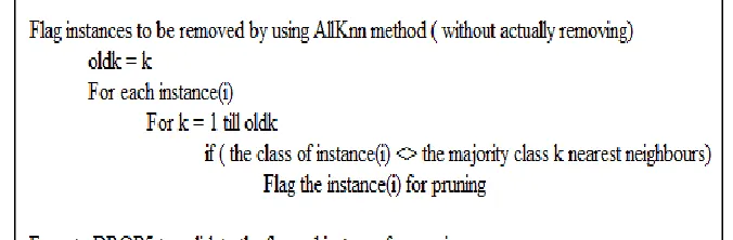
AllKnn (Wilson & Martinez, 1997) is a batch algorithm that makes k iterations. At the ith iteration, it flags as bad any instance that is not classified correctly by its i nearest neighbours. After completing all iterations, the algorithm removes all instances flagged as bad. Figure 3 shows the pseudo code for AllKnn algorithm.
33
Figure 3. Pseudo-code for AllKnn algorithm.
Figure 4. Pseudo-code for DROP5 algorithm.
2.4.1.3 DROP5
DROP5 (Wilson & Martinez, 2000) is a decremental algorithm that removes an instance, “S”, if at least as many of its associates (i.e., instances that have “S” on their NN list) are classified correctly without it. This algorithm removes noisy instances, because a noisy instance, “S”, usually has associates that are mostly of a different class, and such associates will be at least as likely to be classified correctly without “S”.
34
Another method related to the associate set was proposed by Brighton and Mellish (2002), this method is the Iterative Case Filtering algorithm (ICF), based on the Reachable(S) and Coverage(S) sets which are the neighbour and associate sets respectively. ICF discards instance(S) If |Reachable(S)| > | Coverage(S)| which means that some instances in training set (T) can classify instances similar to (S) without considering it in the training set; as initial step, ICF applies ENN. C-Pruner (Zhao et al, 2003) is another method based on the Reachable (S) and Coverage (S). In this method, the Coverage (S) concept only considers the associates with the same class as instance (S) in order to discard instances in the same class. Before discarding an element, this technique determines whether an instance is noisy, superfluous or critical. In this context, an instance is critical when its deletion affects the classification of other instances; in particular, this method discards either noisy or superfluous (but non-critical) instances. When |Coverage (S)| < |Reachable (S)| then “S” is considered as noisy; “S” is superfluous when it is correctly classified by Reachable (S) (Olvera-Lopez et al., 2010).
2.4.2 Rule Induction Pruning
The main weakness with rule learning systems is that they often scale relatively poorly with the sample size of a training set, particularly in the context of noisy data (Cohen, 1993). This is a critical problem due to the prevalence of large, noisy datasets in real-world applications. A variety of methods has been proposed to prune the produced rule sets, and can be categorized as follows:
• Pre-pruning These algorithms either use heuristics (i.e., stopping criteria) to relax the
35
generating a classifier; the hope is that using fewer training examples will produce fewer rules.
• Post-pruning This takes a rule set that is consistent with the training instances and removes
rules and conditions that do not reflect true regularities of domain, such as the Reduced Error Pruning (REP) algorithm (Brunk & Pazzani, 1991) and the GROW algorithm (Cohen, 1993).
• Integration pre-pruning and post-pruning. Instead of learning the entire rule set and
then conducting the pruning, this category prunes a single rule right after the rules have been learned, akin to IREP (Fürnkranz & Widmer, 1994), RIPPER (Cohen, 1995), and Simple Learner with Iterative Pruning to Produce Error Reduction (SLIPPER) (Cohen & Singer, 1999).
2.4.2.1 Pre-pruning
In a rule-induction process, the more conditions we have in the rule, the fewer instances it can cover. Thus, some algorithms employ stopping criteria for noise handling; in addition, to avoid overfitting, there should be a trade-off between covering and accuracy. The pre-pruning for rule inductions can be conducted in two ways:
1. Condition reductions: This can be achieved by pruning each rule independently in the course of learning by using a heuristic to determine when to stop adding conditions to the rule.
36
2.4.2.2 Post-pruning
While pre-pruning algorithms try to avoid overfitting during rule generation (or before applying the rule-induction method), the post-pruning approach initially ignores the problem of overfitting and learns a complete and consistent rule set. It then estimates the quality of this rule set using some quality measurement (usually apparent or Laplace accuracy). If the accuracy can be improved by simplifying the rule set, then this will be repeatedly done until any further simplification would harm the quality of the rule set.
The post-pruning can be done either by checking the effect of removing the condition from each rule and investigating the effect of this removal, or by considering the effect of removing the whole rule from the rule set and checking its effect on the accuracy.
REP is the most common method used for post-pruning. Pagallo and Haussler (1990), Weiss and Indurkhya (1991), and Brunk and Pazzani (1991) employed straightforward adoption of REP to separate and conquer rule-learning frameworks. Initially, the training set is split into two subsets, a “growing set” and a “pruning set”. Then, in the first phase, REP learnsthe concept that covers all positive and no negative examples from the growing set (no attention is paid to the noise in the data). The resulting rule set is then repeatedly simplified by deleting conditions and rules from the set until any further deletion would result in a decrease of predictive accuracy as measured on the pruning set. A variant of REP can employ a variety simplifications to the rule set, such as deleting each condition of a rule, deleting final sequences of conditions1 (Cohen, 1993), or
finding the best replacement condition (Weiss & Indurkhya, 1991).
1 For example, the “if w and x and y and z then class = a” might be simplified to either “if w and x and y then
37
REP for rules usually does improve generalization performance on noisy data (Pagallo & Haussler, 1990), and its search strategy can be regarded as bottom-up as it performs pruning on the resulting rule set. However, it has several shortcomings (Fürnkranz & Widmer, 1994):
• Complexity: REP’s time complexity has been shown to be O (n4) for noisy data, where n
is the number of examples (Cohen, 1993).
• Pruning of conditions in a “separate and conquer” rule will affect all subsequent rules. As pruning conditions from a rule can only generalize the concept – i.e., increase the set of covered examples – a post-pruning algorithm has no means for adjusting the subsequent rules to this new situation. Thus, the learner may be deceived, because the set of examples that remain uncovered by the unpruned rules at the beginning of learning may yield a different evaluation of candidate conditions for subsequent rules compared to the set of examples that remain uncovered by the pruned versions of these rules.
• Generated rules are simplified so that the predictive accuracy on the pruning set will be maximized, but in noisy domains REP will have to do a lot of pruning, and therefore has ample opportunity to get caught in the local maximum.
GROW is introduced to solve some of the drawbacks of the REP algorithm, and replace the bottom-up search of REP with a top-down approach. GROW initially finds a rule set (R0) by overfitting the growing set, then each rule, ri∈ (R0), is taken, and repeatedly simplified in such a
38
set (R0). After the initial rule set (R0) has been expanded, we start with an empty rule set and add rule ri,j from (R0), which improves the predictive accuracy the most on the pruning set. Ties are
broken by choosing the smaller rule. It has been experimentally confirmed that this results in significant gain efficiency on learning time, along with a slight gain in accuracy (Cohen, 1993).
Another methodology for post-pruning is to use Laplace accuracy as a measurement to decide either to remove or retain the produced rules. Sort then Select Rule Reduction (SSRR) (Othman & El Hindi, 2004) concentrates on retaining rules with the highest Laplace accuracy. For each class, it chooses a rule from the produced rule set with the highest Laplace accuracy. Then, it incrementally augments the pruned rule set with all necessary rules in order to make the same classification derived from the original produced rules on the training set. The rules are tried in order, with the one with best Laplace accuracy first. It has been shown (Othman & El Hindi, 2004) that SSRR slightly improves the accuracy in some datasets while achieving good reduction in produced rules.
39
stores R2M in a new rule set (NEW_Rset) and removes it from the RSet. If there are still rules within the RSet that are not processed, the algorithm takes one of them as R2M and repeats the procedure. However, within this approach the NL is specified by the user.
2.4.2.3 Integration pre-pruning and post-pruning
While post-pruning first grows a complete concept description and prunes it thereafter, Fürnkranz and Widmer (1994) proposed a novel learning algorithm called IREP. IREP prunes each individual rule right after it has been generated: after learning a rule from the growing set, the condition is deleted in a greedy fashion until any further deletion would decrease the accuracy of this rule in the pruning set. The resulting rule is added to the concept description and all positive and negative instances covered by the generated rule are removed from the training set “growing and pruning set”. The remaining training set is then split again to form a new growing and pruning set. When the accuracy of the pruned rule is below predictive accuracy of the empty rule (rule with body fail), the rule will not be added to the concept description and IREP returns the learned rule set. The accuracy of an empty rule is N/(N + P), and the accuracy of the pruned rule is (p + (N - n)) / (P + N), where p (n) is the number of positive (negative) examples covered by the rule from a total of P (N) positive (negative) examples in the current pruning set.
40
Experimentally, it seems that GROW outperforms REP, while IREP is better than REP and GROW whenever a fairly general concept has to be found, whereas REP is appropriate when the underlying concept is specific (Fürnkranz & Widmer, 1994).
Cohen (Cohen, 1995) introduced a modification to IREP that allows it to handle multiple classes by placing them in increasing order of prevalence. IREP is then used to find a rule set that separates certain class Ci from the remaining classes. Next, all instances covered by a learned rule set are removed from the dataset. Cohen also introduced some improvements to IREP that enhance its performance. This included three modifications to the IREP algorithm:
1. An alternative metric for assessing the value of the rules in the pruning phase of IREP; 2. A new heuristic for determining when to stop adding rules to a rule set; and
3. A post-process to generate the rules that optimize a rule set in an attempt to more closely approximate IREP.
This is the RIPPER algorithm. RIPPER significantly improves the generalization performance over IREP (Cohen, 1995).
Cohen and Singer (1999) introduced another algorithm similar to the IREP and RIPPER algorithms, called SLIPPER. However, SLIPPER does not remove examples covered by a new rule; instead, it uses boosting to reduce the weight of these examples.
41
metrics used to guide the growing and pruning of rules are replaced with metrics based on formal analysis of boosting algorithms, specifically Freund and Schapire’s (1997) AdaBoot, which employs confidence-rated predictions (Schapire & Singer, 1998).
Other efforts have been applied to generate faster learning. IREP++ (Dain et al., 2004) is one such initiative. It starts by using RIPPER and attempts to develop an algorithm to achieve comparable accuracy by functioning more quickly. The speed improvements are achieved by making several changes to the RIPPER algorithm, including better pruning metrics, a novel data structure, and more efficient stopping criteria. IREP++ (Dain et al., 2004) has been shown to be slightly more accurate than RIPPER, and functioning faster. In addition, IREP++ learns fewer generated rules.
In chapter 5, we compare different rule induction methods based on some important characteristics and choose the methods to be used in our experiments accordingly. Furthermore, we think that the technique of preceding rule induction with instance reduction can achieve a good result with rule induction algorithms which do not use pruning.
2.5 Summary
42
43
Chapter 3: Literature Review: Ant Colony
Optimization
This chapter presents a review of ACO, which is a metaheuristic proposed as a method for solving hard problems, and inspired by the behaviour of real ants.
ACO algorithms are considered to be part of swarm intelligence, which is the study of computational systems inspired by “collective intelligence”. Collective intelligence emerges through the cooperation of large numbers of homogeneous agents in the environment.
This chapter is organized as follows. Section 3.1 presents a formal description of the ACO metaheuristic. Section 3.2 overviews the most popular variants of ACO and gives examples of their application. Section 3.2.1 explains the Ant-Miner algorithm and Section 3.2.2 describes how ACO is applied to feature selection.
3.1 Ant Colony Optimization overview
ACO is a branch of the newly developed form of AI called swarm intelligence. Swarm intelligence is a field that designs algorithms inspired by the collective behaviour of social insects and other animal societies (Bonabeau et al., 1999).
The potential benefits of imitating social insects’ structural models and behaviour in designing solutions to a problem include:
44
• Flexibility, in terms of adaptation to changing environments.
In groups of insects that live-in colonies, such as ants and bees, individuals can only accomplish simple tasks on their own, while the colony, working cooperatively, can perform complex tasks. Ants also have the ability to find the shortest path from their nest to a food source. When a food source is first located, several ants may have taken several different paths to reach that food source. When an ant moves, it lays a chemical substance called a pheromone along its path. When foraging for food and taking it back to its nest it follows the path with the greatest amount of a pheromone laid upon it. Pheromone trails evaporate if more ants do not come along to reinforce it, and ants that find the shortest route to the food will arrive back at the nest quicker than others; thus, the greater the number of ants on one path, the greater the amount of pheromone on that path. When new ants seek to travel to the food source they then take the shortest route (since they are guided by the amount of pheromone on the path). It has been observed that all foraging ants eventually converge on the shortest route to the food source (Galea, 2002).
ACO is a technique used with combinatorial optimization problems, which consist of finding an optimal solution from a finite set of solutions. In many such problems, exhaustive search is not feasible. There are, however, some important differences between real and artificial ants (Socha, 2008):
• Artificial ants live in a discrete world – they move sequentially through a finite set of problem states.
45
is carried out only by some of the artificial ants, and often only after a solution has been constructed.
• Some implementations of artificial ants use additional mechanisms that do not exist in the case of real ants. Examples include look-ahead, local search, backtracking, etc.
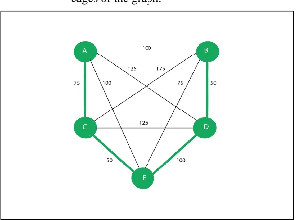
The first ACO was developed by Marco Dorigo and published under the name of Ant System (AS) in (Dorigo et al., 1996). The application was the traveling salesmanproblem (TSP), which is classified as NP-hard combinatorial optimization because the solution cannot be found in polynomial time. The goal of TSP is to find the shortest possible route through a set of connected (N) cities, with each city visited once and only once. The ants find a solution to the TSP by traversing a problem graph from one city to another, depositing pheromone, until they solve the TSP. During an iteration of the AS algorithm, each ant builds a tour comprising N steps:
For each ant, the transition from city i to city j depends on: 1. Whether the city has been visited.
2. The inverse of distance α = 1/dij, which is based on local information and represents
the heuristic desirability of choosing city j when in city i.
3. The amount of pheromone trail, µij, on the edge connecting city i to city j.
ACO can solve any problem for which the following elements can be defined (Socha, 2004):
46
have a fully connected weighted graph, where the set of nodes, N, represent the cities and the set of edges represent the connection between the cities, as shown in Figure 5.
2. A local heuristic provides guidance to the ant in choosing the next node for the path it is building. In the TSP, the local heuristic is the inverse of distance, which represents the heuristic desirability of choosing city j when in city i.
3. The probabilistic transition rule determines which node an ant should visit next. The transition rule is dependent on the heuristic value and pheromone level associated with an edge joining two nodes.
4. A fitness function determines the fitness of the solution built by an ant in the TSP, where the fitness function is the length of the whole path traversed by the ant. 5. A pheromone update rule specifies how to modify the pheromone trail laid along
[image:46.612.72.371.412.634.2]edges of the graph.
Figure 5. A weighted graph for TSP with five cities.
47
initially set to be equal to 1. The initial visibility for each city is the inverse of the distance between the cities. Thus, the probability of choosing cities B, C, D and E are:
P1 AB =
1/100
(1001 )+(751)+(1001 )+(1251 ) = .242
P1AC = .323
P1AD = .194
P1AE = .242
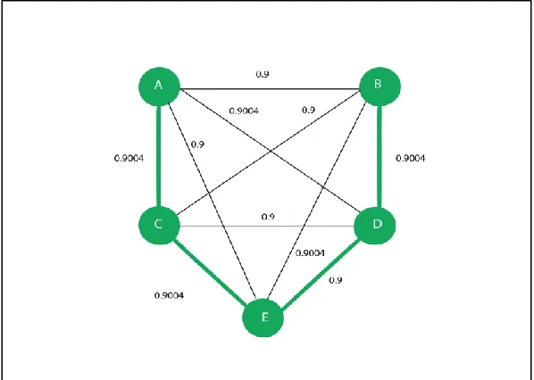
Therefore, the ant chooses to visit city C. Continuing the iteration, the ant completes the tour by visiting the cities E, B, and D, in that order, for a tour of length 250. After completing the tour, the ant lays pheromone along the path of the tour. The amount of pheromone added is equal to the inverse of the total length of the tour. Thus,
∆
µ
=1
75+50+75+50 = .004
Furthermore, the pheromone is decreased along all edges to simulate pheromone decay according to the pheromone evaporate rate. The pheromone for the edges in the path is therefore updated by (assuming that the pheromone evaporate rate is 0.1):
µ
= (1- .1) + .1 (.004) = .9004.And the pheromone for edges not in the path will be updated by,
µ
= (1- .1) + .1 (0) = .9.48
Now, the total length of the tour is 275, and hence this tour is taken as the shortest path so far (when the starting point is city B). The pheromone updates are completed as earlier. The algorithm continues to find the shortest path until the terminating condition is met, which is a certain number of solution constructions fixed at the beginning of the algorithm.
[image:48.612.72.371.315.528.2]The great advantage of ACO over the use of exact methods is that the ACO algorithm provides relatively good results via a comparatively low number of iterations, and is therefore able to find an acceptable solution in a comparatively short time.
Figure 6. Pheromone values for the structure shown in Figure 5 after the first ant finishes a tour.
49
3.2 Application of ACO to Classification Rule Induction
Parpinelli et al. (2002) were the first to propose using ACO to discover classification rules with the Ant-Miner system; they argued that an ant-based search is more flexible compared to traditional methods.
Ant algorithms simulate the foraging of real ants, so it is a good idea to think about the problem as a search for a best path through a graph, where the nodes represent the partial solution and edges represent the transition between these partial solutions. The edge labels are measurements that qualify the selected partial solutions.
In this section, we will review two interesting applications for ACO that have achieved good results in their field. We will demonstrate how ACO has been applied to solve these kinds of applications.
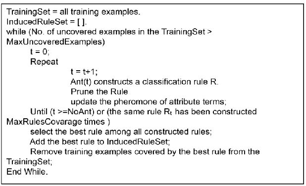
3.2.1 Ant-Miner Algorithm
50
Figure 7. Ant-Miner algorithm.
When applying the Ant-Miner algorithm to classification rule induction, the basic element of the solution is attribute terms. An attribute term, termij, is in the form Ai = Vij, where Ai is the
ith attribute and Vij is the jth value of domain A. Thus, an appropriate problem for ACO
representation regarding the induction of classification rules is a graph whose nodes represent attribute terms. A complete path is a constructed rule, and the quality of the path is assessed by a global2 fitness function. The quality of node is evaluated by heuristic value and pheromone level
value associated with the node.
In Ant-Miner, each ant starts with an empty rule – i.e., with no term in its rule antecedent – and adds one term at a time. The choice of term to be added to the current partial rule antecedent depends on both the heuristic value (based on term entropy) and the pheromone level associated
2 The scope of the global fitness function extends only to the current constructed rule, and not to full execution of
51
with each term. The entropy in Ant-Miner is computed for a specific attribute value, which is defined by:
H (C| A
i= V
ij) = -
∑
𝑃(𝑐|𝐴
𝑖= 𝑉
𝑖𝑗) ∗
𝑘
𝑐=1
𝑙𝑜𝑔
2𝑃(𝑐|𝐴
𝑖= 𝑉
𝑖𝑗)
(7)Where:
c is the class attribute and k is the number of class values.
Ai is the ith attribute and Vij is the jth attribute value of the ith attribute.
P(c | Ai = Vij) is the probability of observing class c, conditional on observing Ai = Vij.
The higher the entropy value of a term, the more uniformly distributed the classes are, and, thus, the smaller the probability that the current ant chooses this term to add to its partial rule. In Equation 8, H (C| Ai = Vij) is subtracted from 1 because the ant is seeking a term that will
distinguish between the class values, since it is building a classification rule. The entropy values are normalized using Equation 8 (Swaminathan, 2006).
Ħ
ij=
(1 − 𝐻(𝐶|𝐴
𝑖= 𝑉
𝑖𝑗))/(∑
𝑎𝑙=1𝑥
𝑙∗
(1 − ∑
𝐻 (𝐶|
𝑏𝑖
𝑚=1
𝐴
𝑙= 𝑉
𝑙𝑚)))
(8)a is the total number of attributes.
xl is set to 1 if attribute Al has not yet been selected; otherwise, it is set to 0.
bi is the number of domain values for ith attribute.
52
transition rule gives the probability of adding the attribute–value pair to the rule. The one with highest probability is added to the rule.
P
ij=
(Ħ
𝑖𝑗∗ µ
𝑖𝑗(𝑡))/(∑
(𝑥
𝑙∗
𝑎
𝑙=1
∑
𝑏𝑖
𝑚=1
Ħ
𝑙𝑚∗ µ
𝑙𝑚(𝑡)))
(9) Where:Pij is the probability that termij is selected for addition to the current partial antecedent.
Ħ ij is the heuristic value associated with termij.
µij (t) is the amount of pheromone associated with termij at iteration t.
a is the total number of attributes.
bi is the number of domain values of the ith attribute.
xl is set to 1 if attribute Al has not yet been selected; otherwise, it is set to 0.
Once an ant has stopped building a rule antecedent, a rule consequent is chosen. The rule consequent is assigned the class label of the majority class among the instances covered by the antecedent.
53
sensitivity) and accuracy among negative examples (called specificity). Thus, the quality of the rule is defined by the following:
Q =
𝑇𝑃+ 𝐹𝑁𝑇𝑃∗
𝐹𝑃+ 𝑇𝑁𝑇𝑁 (10)Where:
TP, true positive, is the number of examples covered by the rule that belong to the class predicted by the rule.
FP, false positive, is the number of examples covered by the rule that belong to a class that is different from the class predicted by the rule.
FN, false negative, is the number of examples that are not covered by the rule, but that belong to the class predicted by the rule.
TN, true negative, is the number of examples that are not covered by the rule and do not belong to the class predicted by the rule.
Other variations from Ant-Miner use Laplace accuracy to estimate the constructed rule. It has been observed that Ant-Miner achieves better prediction accuracy when using Laplace accuracy, compared to using the sensitivity/specificity fitness function (Xuepeng, 2004).
Once rule pruning is complete, the pheromone levels are updated for the terms by increasing the pheromone for the terms that appear in the rule antecedent according to the rule quality given by:
µ
ij(t+1) = µ
ij(t) + µ
ij(t) * Q.
(11)Where
µij (t) is the pheromone level of termij.
54
The ant then normalizes the pheromone level of all terms (each pheromone level is divided by the sum of all pheromone levels), which reinforces the pheromone levels of the terms occurring in the rule antecedent and decreases the pheromone levels of other terms that are not selected in the rule.
The process by which an ant creates a rule is repeated for, at most, a predefined number of ants. However, the process may stop if the current ant has just created a rule that is exactly the same as a previous (maxRulesConverge -1) rule. MaxRulesConverge is a user-defined parameter for testing the convergence of ants, which simulates the convergence of real ants to the shortest path between a food source and their nest. The best rule created is added to the InducedRuleSet, the training set is appropriately reduced, and another run generates a best rule to cover more instances from remaining training instances.
55
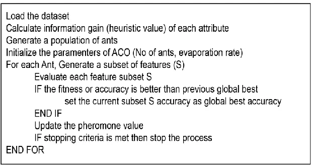
3.2.2 Feature Subset Selection
Feature subset selection is a method for selecting a subset of relevant features in order to generate good classifiers. The importance of the feature subset selection technique lies in its ability to provide a better understanding of the data and reduce the training time of the learning algorithm, because it helps in reducing the complexity of a given training set. It is computationally expensive and infeasible to implement feature subset selection via exhaustive evaluation of all possible subsets, especially as there may be thousands of features present in real-world datasets.
The feature subset selection algorithms can be categorized into two groups:
1. The filter approach, which is a feature subset selection technique applied independently of the learning algorithm. These methods apply some ranking over features. The ranking denotes how ’useful’ each feature is likely to be for classification. a number of performance criteria have been proposed for filter-based feature selection such as fisher score (Duda et al., 2012), methods based on mutual information (Koller & Sahami, 1996) and ReliefF (Kira & Rendell, 1992).
2. The wrapper approach, wherein the evaluation criteria is tied to the learning algorithm. It considers feature subsets by the quality of the performance on a learning algorithm, which is taken as a black box evaluator. (e.g. Naïve Bayes or SVM) (Maldonado et al., 2014).